Smooth Path Planning of a Mobile Robot Using Stochastic Particle Swarm Optimization
- 格式:pdf
- 大小:244.27 KB
- 文档页数:6
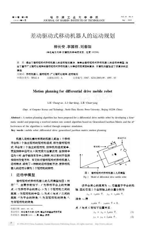
第35卷 第9期2003年9月 哈 尔 滨 工 业 大 学 学 报JOURNA L OF H ARBI N I NSTIT UTE OF TECH NO LOGYV ol 135N o 19Sep.,2003差动驱动式移动机器人的运动规划柳长安,李国栋,刘春阳(华北电力大学计算机科学与技术系,北京102206)摘 要:提出了差动驱动式移动机器人的运动规划算法.推导出差动驱动式移动机器人的运动学模型,给出了基于广义雅可比矩阵的差动驱动式移动机器人分解运动速度控制算法.计算机仿真验证了该算法的正确性.关键词:移动机器人;差动驱动;广义雅可比矩阵;运动规划中图分类号:TP24216文献标识码:A文章编号:0367-6234(2003)09-1095-03Motion planning for differential drive mobile robotLI U Chang 2an ,LI G uo 2dong ,LI U Chun 2yang(Dept.of C om puter Science and T echnology ,N orth China E lectric P ower University ,Beijing 102206,China )Abstract :A m otion planning alg orithm has been proposed for a differential drive m obile robot by developing a kine 2matic m odel and proposing a res olved m otion rate control alg orithm based on G eneralized Jacobian Matrix and the ef 2fectiveness of the alg orithm is verified through com puter simulation.K ey w ords :m obile robot ;differential drive ;generalized jacobian matrix ;m otion planning收稿日期:2003-05-01.基金项目:华北电力大学(北京)博士科学基金资助项目.作者简介:柳长安(1971-),男,博士,讲师. 机器人足球比赛所采用的机器人都由1个移动平台和2个独立驱动的驱动轮组成,称为差动驱动式.平台有2个独立的驱动轮,该种机构组成简单,而且旋转半径可从0到无限大任意设定.当旋转半径为0时,由于能绕本体中心旋转,所以有利于在狭窄场所改变方向.本文针对差动驱动式移动机器人运动特点,研究了一种新的运动控制方法,使移动机器人的运动分解为2个驱动轮的转动.1 运动学模型差动驱动式移动机器人的几何模型如图1所示[1,2].主要参数如下:F 为移动平台上的关键点;G 为移动平台的质心;b 为2个驱动轮之间的距离;r 为驱动轮的半径;l G 为点G 与点F 之间的距离;<为平台的转角;θl 为左驱动轮的转角;θr 为右驱动轮的转角.图1 差动驱动式移动机器人几何模型Fig.1 M odel of differential drive m obile robot 设平台质心的速度为v G ,它垂直于平台的轮轴,因此它在2个坐标轴上的分量分别为x G =v G cos <, y G =v G sin <,消去v G 得x G sin <-y G cos <=0.点F 与点G 有如下位置关系:x F =x G +l G cos <,(1)y F =y G +l G sin <.(2)对式(1)、(2)求导可得 x F = x G -l G <sin <, y F = y G +l G <cos <.F 点的速度关系可以表示为x F sin <- y F cos <+l G <=0,平台质心的速度与驱动轮转速的关系式为<= θr r - θl r b ,v G =r2( θl+ θr ),可以得到矩阵表达式为x Fy F <=r2c os <+l G rbsin <r2c os <-l G rbsin<r2sin <-l G rbc os <r2sin <+l G rb c os <-rbrbθl θr,从而得P ・=J Φ・.(3)式中:P ・=x F y F <T ;Φ・= θl θrT;J =r2cos <+l G rbsin <r 2cos <-l G rb sin <r2sin <-l G rb cos <r2sin <+l G rbcos <-r br b.J 定义为差动驱动式移动机器人的广义雅可比矩阵,它与基座固定的机械手雅可比矩阵类似,反映差动驱动式移动机器人关键点的速度与驱动轮转速之间的关系.2 分解运动速度控制由式(3)可知,给出机器人驱动轮转速可以求出机器人上关键点的速度,给出移动机器人关键点的速度也可以求出驱动轮转速,这时驱动轮控制量可由下式给出:Φ=J -1 P .采用计算机控制,速度项可以表示为单位时间里(控制周期Δt )的位移增量,即ΔΦ=J -1ΔP .(4)式中:ΔP 为一个控制周期内的位移变化;ΔΦ为同一时间间隔内的角度变化.如果给定F 点的轨迹,当Δt 选定时,可以确定ΔP ,将其代入式(4)求出各个角度增量ΔΦ,可得到各个角度的给定值,最后由角度伺服控制系统去实现位置控制,这就是分解运动速度控制.差动驱动式移动机器人的分解运动速度控制是一种基于逆广义雅可比矩阵的连续路径跟踪控制方法[3,4].该算法要考虑合理的控制周期.分解运动速度控制方法通过控制每个周期内的角度输出量实现对轨迹的跟踪或速度控制.如果控制周期选择的太大,则运动控制的精度难以达到要求,如果控制周期选择过小,在每个周期内都要计算逆矩阵,给实时控制造成困难[5].具体算法描述如下:步骤(1):输入机器人的初始状态信息.平台质心的位置为r G (0),平台的方向角为<(0),驱动轮的转角θl (0)=0、θr (0)=0,置i =0.步骤(2):输入点F 的轨迹x F =f 1(t )、y F =f 2(x F ).确定控制周期Δt ,并把整个运动过程分为N 步完成.步骤(3):确定该周期的ΔP ,计算ΔΦ(i )=J -1ΔP (i ),确定该周期内的ΔΦ(i ).步骤(4):按照ΔΦ(i )驱动机器人运动.步骤(5):确定系统的新状态.平台质心的位置为r G (i +1)=r G (i )+Δr G ,平台的方向角为<(i +1)=<(i )+Δ<,驱动轮的转角为θl (i +1)=θl (i )+Δθl (i ),θr (i +1)=θr (i )+Δθr (i ).步骤(6):if (i =N )转步骤(7),否则i =i +1,转步骤(3).步骤(7):结束.3 计算机仿真为了验证本文提出的差动驱动式移动机器人运动规划算法的正确性和可行性,在I BM -PC 机上进行了计算机仿真,仿真软件采用MAT LI B 可视化编程工具.机器人系统的参数选择半自主足球机器人的实际参数,其中b =01075、l G =010375、r =0101875.初始条件为(x 0F ,y 0F ,<0)=(011,015,90°);终了条件为(x n F ,y n F ,<n )=(016,011,0°).假设F 点的轨迹为x F =a 1t +a 0,y F =b 1(x E )3+b. 设整个运动过程用时间为10s ,取Δt =0105s.图2给出了机器人平台上关键点的理想运动轨迹,图3给出了移动机器人的运动过程仿真结果.从仿真结果可以看出,差动驱动式移动机器人运用该控制算法分别驱动2个驱动轮转动可以实现机器人上关键点跟踪预定轨迹,同时也能完成机器人方向角的改变.・6901・哈 尔 滨 工 业 大 学 学 报 第35卷 图2 移动机器人的理想运动轨迹Fig.2 Desired path of m obile robot图3 移动机器人运动过程的仿真结果Fig.3 Animation of m otion of m obile robot 4 结 论(1)该算法是一种基于广义雅可比矩阵的分解运动速度控制算法,使移动机器人的运动分解为驱动轮的转动.(2)利用该算法应该考虑合理的控制周期.如果控制周期选择的太大,则运动控制的精度难以达到要求;如果控制周期选择过小,则计算速度慢,给实时控制造成困难.(3)该算法很好地解决了差动驱动式移动机器人系统的运动规划问题,为研究此类系统的动力学问题奠定了基础.参考文献:[1]蔡自兴.机器人学[M].北京:清华大学出版社,2000.[2]白井良明.机器人工程[M].北京:科学出版社,2001.[3]薄喜柱.基于多智能体合作的机器人足球比赛系统的研究[D].哈尔滨:哈尔滨工业大学,2001.[4]洪炳熔.机器人足球比赛-发展人工智能的里程碑[J].电子世界,2000(4):4-5.[5]SER J I H.A unified approach to m otion control of m obile ma2nipulators[J].The International Journal of R obotics re2 search,1998,17(2):10-15.(编辑 王小唯)(上接第1094页)适应值函数的影响,否则进行惩罚———取负值,使适应值减小.通过f来评价路径在遗传过程中的适应值,f越大,路径的优化程度越高.113 遗传操作步骤(1)根据编码方案,把路径点编码成位串形式,转化为染色体(路径).(2)选择合适的参数:群体的大小(所含个体数M)、交叉概率p c和变异概率p m.(3)随机产生一个初始群体即M条路径.(4)根据适应值函数计算每条路径的适应值f i,并计算群体的总适应值F=Σf i,i= 1……M.(5)选择:计算每一条路径的选择概率p i=f i/F及累计概率q i=Σp j,j=1,…I.(6)交叉:对每条路径产生[0,1]间随机数r,如果r<p c,则该条路径参加交叉操作,如此选出参加交叉的一组路径后,随机配对;对每一对,产生[0,1]间的随机数以确定交叉的位置.(7)变异:如果变异概率为p m,则可能变异的位数的期望值为p m・m・M(m为染色体串长,M 为群体).(8)如果新个体数未达到M个,则转向第(5)步继续进行遗传操作,否则代数加一,d=d+1;将新群体的M条路径的适应值由大到小进行排序;保存适应值最大的路径点,如果d≠g(g是设定的代数),则转向第(4)步,否则选用g代中f 值最好的路径上的点.2 结 语在仿真足球机器人的决策系统中进行了实验,在实验中,选择与同一支队伍进行比赛,使用同一种战术,进行40场比赛,在应用遗传算法避障后,每10场的平均进球数增加了近2个.本文中介绍的基于遗传算法的回避多个障碍的路径规划策略通过仿真系统和实赛的检验,显示出良好的效果,取得了可喜的成绩.(下转第1101页)・791・第9期柳长安,等:差动驱动式移动机器人的运动规划运动方程为I1I 2…I 6p =J 1a…0J 1u 0…J 2aω…0J 2uω……ωω0…ωω0…J 6a…J 6u q 1aq 2a …q 6a q 1uq 2u …q 6u ,或者A 0 p =B 0p q p .式中:A 0为24×4矩阵; p 为4×1矩阵RV XRRV YRRV ZRRωZRT,代表月球车的期望速度值和车体方向值;B 0p 为24×96的块对角矩阵;q ・p 为96×1矩阵,为待求解的可执行月球车变量;q ・ia 表示月球车可执行的变量数;q ・iu 表示月球车不需执行的变量数.采用最小二乘法,可执行的月球车变量的反向运动解为q a =[J T 1aJ 1a ]-1J T 1a[J T2a J 2a ]-1J T2a …[J T6a J 6a ]-1J T6ap .(7) 通过式(7)可以求得月球车的48个可执行变量.本文所叙述的月球车的逆运动学求解依赖月球车的位型假定,一般而言,在崎岖地形中移动的多轮机器人的逆运动学数值解都是有效解.2 结 论(1)该方法不仅能描述车体在崎岖地形中6个自由度的运动变化,得到车体速度的最优解,而且能够在存在传感噪声和车轮滑移情况下估推月球车的位置和方向,便于月球车的路径规划和自主导航.(2)逆运动学求解方法通过将地形等高图、月球车运动的期望位置和方向作为输入,得出月球车在地图中给定点的稳定性和可穿越性,便于月球车的运动控制.参考文献[1] M UIR P F ,NE UM ANN C P.K inematic m odeling ofwheeled m obile robots[J ].J R obotics Systems ,1987,4(2):281-340.[2] A LEX ANDER J C ,M ADDOCK SJ H.On the kinematic ofwheeled m obile robots [J ].Int J R obotics Research ,1989,8(5):15-26.[3] T AROK H M ,MC DERM OTT G,H AY ATI S ,et al .K inematic odeling of a high m obility mars rover [A ].International C on ference on R obotics and Automation [C].Detroit :M ichigan ,1999.[4] I AG NE M M A K,SHI BLY H ,RZEPNIEWSKI A ,et al.Planning control alg orithms for enhanced rough -terrain rover m obility [A ].Proceeding of the 6th International Sym posium on Artificial Intelligence and R obotics and Automation in S pace [C ].Quebec :Canadian S pace A 2gency ,S t -Hubert ,2001.[5] I AG NE M M A K,RZEPNIEWSKI A ,DUBOSKY S ,et al.C ontrol of robotic vehicles with actively articulated sus 2pensionsin rough terrain[J ].Autonom ous R obots ,2003,14:5-16.[6] I AG NE M M A K,RZEPNIEWSKI A ,DUBOWSKY S ,etal.M obile robot kinematic recon figurability for rough -terrain[A].Proceedings of the SPIE Sym posium on Sen 2s or Fusion and Decentralized C ontrol in R obotic Systems III[C].Boston :[s.n.],2000.(编辑 王小唯)(上接第1097页)参考文献:[1]金 玺.基于仿真机器人足球平台的多智能体控制研究[D].北京:北京理工大学,2003.[2]ARAU T ,OT A J.M otion planning of multiple m obile robots[J ].IEEE Proc Int C on f on Intelligent R obots and System ,1992:1761-1768.[3]薛宏涛,沈林成,常文森.PTS 领域中的Agent 体系结构设计与实现[J ].计算机工程与应用,2000,36(7):76-78.[4]H ONG Bing 2rong.R obot s occer simulation com petition plat 2form based on multi 2agent [M].[s.l.]:FIRA -K AIST Cup W orkshop ,2002.[5]李 实,徐旭明,叶 榛.机器人足球仿真比赛的S erver模型[J ].系统仿真学报,2000,12(2):138-142.(编辑 王小唯)・1011・第9期蔡则苏,等:HIT -1型月球车的运动学分析。

移动操作机器人及其共享控制力反馈遥操作研究博士学位论文移动操作机器人及其共享控制的力反馈遥操作研究RESEARCH ON MOBILE MANIPULATOR AND ITSFORCE FEEDBACK TELEOPERATION BASED ONSHARED CONTROL MODE于振中哈尔滨工业大学2010年 11月国内图书分类号:TP242.2学校代码:10213国际图书分类号:681.5 密级:公开工学博士学位论文移动操作机器人及其共享控制的力反馈遥操作研究博士研究生 :于振中导师 :蔡鹤皋院士副导师 :赵杰教授申请学位 :工学博士学科 :机械电子工程所在单位 :机电工程学院答辩日期 : 2010 年 11 月授予学位单位 :哈尔滨工业大学Classified Index: TP242.2U.D.C: 681.5Dissertation for the Doctoral Degree in EngineeringRESEARCH ON MOBILE MANIPULATOR AND ITSFORCE FEEDBACK TELEOPERATION BASED ONSHARED CONTROL MODEYu ZhenzhongCandidate:Supervisor: Academician Cai HegaoVice-Supervisor: Prof. Zhao Jie Academic Degree Applied for: Doctor of EngineeringSpeciality: Mechantronics EngineeringUnit: School of Mechatronics EngineeringDate of Defense: Nov, 2010University: Harbin Institute of Technology摘要摘要移动操作机器人相比于固定操作机器人具有更大的操作空间和更强的操作灵活性,成为机器人领域研究的热点方向之一。

Abstract—This paper presents the use of search algorithms and discrete environments to find the path in mobile robots systems navigation. Implementations of Breadth-First search algorithm are made both in software and in hardware. The results using the hardware approach provide significant time gain, compared with the software implementation. The time gain and the dynamical hardware reconfigurability allow multiple tasks implementation and the possibility to choose the appropriate one for the application.Index Terms— hardware design, mobile robots, path planning, search algorithms.I.INTRODUCTIONMobile robots systems are driven by control systems. The architecture of these control systems provides different blocks to accomplish specific robotic tasks. Traditionally, the research in the field of Robotics is focused on the algorithms used to accomplish fundamental tasks, like path planning [1]. The path-planning task, part of a mobile robot navigation system, involves searching and finding the path between a Start Point and a Goal Point in the environment where the robots navigate. The environment is static or dynamic and may have a discrete or continuous representation. Mobile robots need to avoid obstacle collisions and generate an optimal result with respect to path dimension or to execution time. These imply different possible implementations [2].To reach the goal, mobile robots need to have the ability to act as to assure an efficient and reliable navigation. A great variety of approaches for this strategic task have been experimented [3].The approaches that solve path planning are generally based on software implementation. There are only a few hardware implementation directions that have demonstrated navigation competence [4].Nowadays the Field Programmable Gate Array (FPGA) circuits and other hardware reconfigurable systems makes it possible to achieve implementations with a degree of flexibility that only software applications were considered to have until now. FPGA circuits allow running high-speed hardware applications and provide a high degree of parallelism [5].While the quantity and diversity of the environments increases, the criteria and applications that imply huge computing power consumption for the mobile robots navigation continue to increase, the encapsulated real-time architectures for the mobile robots navigation systems must respond with flexibility and enhanced processing capacity and performance. Many repeating and time-consuming operations are adequate to be implemented in reconfigurable hardware. The establishment of a frame within which the hardware applications can be dynamically reconfigured to respond to the real-time requirements would allow new criteria approaches in robot applications [6].The search algorithms represent a useful and reliable technique in solving path-finding, path-planning and obstacle-avoidance types of problems. They are successfully used to determine a valid path [7].The basic idea of our approach is to highlight differences between software and hardware implementations of path generation from a Start Point to a Goal Point, path that will be followed by mobile robots. At the same time we show that the hardware approach provides significant time gain and also easy and fast switching between multiple algorithms. We started using the Breadth-First (BF) algorithm to obtain the path generated in a given static discrete environment. Implementations are made both in software and in hardware. The paper is structured as follows: section 2 deals with the overall description of BF used algorithm and its software implementation and results. Section 3 explains the hardware implementation chosen for the algorithm and presents the tests and experimental validation. Section 4 reports the comparative results obtained by the two implementations, and shows conclusions and ideas for future work.II.SOFTWARE IMPLEMENTATIONThe environment where the path planning is made is one with a typical bi-dimensional discrete representation. Most often it is represented as a matrix of squares (cells), and denotes the positions of the cells using the combination of theMobile Robot Path Planning Software and Hardware ImplementationsLucia Vacariu, Flaviu Roman, Mihai Timar, Tudor Stanciu, Radu Banabic, Octavian Cret Computer Science Department, Technical University of Cluj-Napoca, Romania{Lucia.Vacariu, Octavian.Cret}@cs.utcluj.rotwo coordinates. This way, the environment presents the cells as Nodes, and each node has neighbors in 4 directions (N, S, W, E). There is no connection on diagonals. The dimension of the matrix is known. The matrix contains free spaces, static obstacles, the Starting Point (S) and the Goal Point (G). It is assumed that the matrix is closed, bordered by obstacles. There are several algorithms used to obtain a path in such environments. In a finite environment all the algorithms assure that a path will be found between the Start Point and the Goal Point. The characterization of algorithms is made with respect to the length of the generated path and with respect to the time spent to obtain it. These two criteria are independent. The shortest path does not necessarily imply the minimum time, or vice-versa.By implementing path planning algorithms and their alternative usage with respect to the application demands, we aim to obtain an optimal path and minimum execution time. A.Breadth-First Search AlgorithmWe start using the Breadth-First (BF) algorithm to obtain the path. BF is a technique for searching and returning a path from a given Starting Point to a given Goal Point. The algorithm guarantees finding a solution, if there exists one. As for its complexity, it is a linear algorithm with respect to the number of considered nodes, while the way it searches is based on maintaining a queue of all neighbors found to be accessible through means of vertices until the Goal is reached. Keeping a similar queue, in which for each node we keep the one from which our node was found as neighbor, makes it possible to reconstruct the path.Given a random map of the environment, that respects the criteria mentioned above, a Starting Point and a Goal Point, the implementation of BF will return (if there exists) a valid path between the two points. The path will be marked, assuming that one can pass only through the free spaces and the directions of motion are only the ones stated. The algorithm is presented in Listing 1.The reconstruction of the solution is done by means of a special routine, which takes the list of previous elements and reconstructs the visited points of the map (Listing 2).B.Implementation and resultsFor the software implementation and experiments, we have chosen Java as programming language. The implementation required Object-Oriented techniques, Graphical User Interface and Data/Maps saving and exporting, the Java compiler and emulator [8], and the Eclipse IDE [9]. The tests were performed on an Intel Pentium M at 1.73GHz, with 1G RAM. The procedure to measure the time interval in which the algorithm runs was to capture the system time and to compute the difference of the values before and after the execution of the algorithm routine (Listing 3).We performed various tests on manually generated maps, random maps, and small to large maps. The maps are displayed using Black for obstacles and White for free spaces. The starting point is Blue, and the goal is Yellow. We observed that the running time increases significantly for large maps. Each increase in the length of an assumed square matrix produces a 2nd order polynomial increase (with respect to the matrix dimension) in the execution time, because of the spreading (the cells included in the search queue but which arenot on the final path).Listing 1. BF Search AlgorithmListing 2. Reconstruction of pathListing 3. Execution time computingResults prove very short paths (80% of the times optimal) and fast times only for small matrices (Fig.1.).Fig.1. 10x10 map dimensionFor larger maps (e.g. 100x100 cells) the time increases verymuch (Fig.2).Fig.2. 100x100 map dimensionA comparison table (Table 1.) has been generated, based on the obtained time and the spreading results. A larger spreading implies larger execution time because the spreading is included in the search queue, so each node is expanded. For same dimension maps, but with fewer obstacles, the execution time was greater. This is because a less obstacle-filled map generates a larger spreading. The time is given inmicroseconds.Table 1. Software BF implementation resultsIII. HARDWARE IMPLEMENTATIONOur hardware-based environment is built upon Xilinx FPGA core technologies, which is the well-known developing technology in reconfigurable-based computing functionalities.A. Hardware DesignFor the hardware implementation, we chose from the FPGA family, a Xilinx Virtex 2Pro Board (XC2VP30-FF896-6),manufactured by Digilent Inc. The board is equipped with VGA-output, used for visualizing test results on the monitor.It required Xilinx ISE 8.1 Environment [10], which was used for VHDL code synthesis, implementation and board programming.For the hardware implementation, a series of adaptations of BF algorithm had to be done, in order to exploit the logic resources of the Virtex FPGA device. The input matrix is stored in BlockRAMs. Depending on the space available in the FPGA device, the process memory can be implemented inside or outside the chip (in the Virtex BlockRAMs or in an external Dynamic RAM).All components have been described in parameterizable VHDL code. Thus, the design becomes portable on any hardware support system.1) Components design: The hardware solution is based on a structural description with component-style design. It uses interconnected components, each of them performing a certain task. The most important component is the BF component,which implements the algorithm (Fig.3.).Fig.3. BF componentThe signals interact with the required memory for applying the BF algorithm, while some of the signals (clock , solve as inputs and ready as output) are signals that belong to the hardware configurations and interconnections.To implement the memory, FPGA Virtex BlockRAMs were used. This way, the speed of the configuration increases because specialized components are used, and also the number of available Virtex slices makes it possible to implement larger designs.As mentioned in Section II, the BF algorithm uses a structure that retains all the neighbors of the current element.In our case this structure is implemented in hardware by an array, and uses more auxiliary array signals, all stored in BlockRAMs. BF uses the start and target signals to identify the position in the neighbors’ structure. It also contains a direction signal, which is the most important, as it points to the direction in which the algorithm searches for emptyspaces. This signal is looped in the 0-3 sequence, pointing to the 4 directions.As a final result, BF will set the algorithm path to Red.Spreading will be marked with Green. The starting point is Blue, and the goal is Yellow. Here Black is for free spaces and White is for obstacles.The MarkPath component is the one that implements the reconstruction of the path after the algorithm has been applied(Fig.4.).Fig.4. MarkPath ComponentIn hardware, no initialization of values is made automatically, therefore it is required that before any algorithm is applied, the system is brought to an initial known state, which must be a beginning state for the algorithm. Every signal must be initialized, and the memory map also. The component that deals with all these and with other clock synchronization and enable / ready types of signals is calledCentralUnit (Fig.5).Fig.5. CentralUnit ComponentThe Serial component implements the interface that assures the receiving and transmission of the information from / to the computer through the serial port connection. The data format use: 1 start bit; 8 data bits; 1 parity bit; 1 stop bit. The environment map is received and the path given by thealgorithm is transmitted (Fig.6.).Fig.6. Serial ComponentThe VGA module contains the necessary signals to synchronize the output on a regular monitor (the VGA controller that provides the image on an 800x600 pixels screen display). The component captures the value from the matrix, which represents the type of cell to be displayed, and it outputs the color corresponding to the value (Fig.7). Thematrix acts like a video memory for the component.Fig.7. VGA Component2) Integrated system: The architecture of integrated system has been designed as the collection of components. The connection between components is made by relatively simple Finite State Machines (FSM’s), by signals, and with a few processes that handle the synchronization, command all the components, acquire signals from board inputs, and send datato outputs (Fig.8.).Fig.8. Integrated systemB. Hardware ResultsTo test the hardware implementation we used the same maps that were used for the software implementation. The system was tested several times to verify its reliability.The path found after BF algorithm execution was displayed on the monitor and was photographed in different stages of evolution. We used these pictures to compare them with the results from the software implementation.The path is also saved in a file on the computer, after transferred through the serial port, and is used in the navigation system of the mobile robot.At the beginning, after running Xilinx Synthesis software for our hardware implementation, the report indicated a maximal working frequency of 185 MHz (clock period: 5.4ns).The space available in FPGA Virtex devices allows the implementation of a large matrix (e.g. 100x100). Our maps use variable dimension matrices. The report generated by Xilinx synthesis tool shows that the FPGA circuit is used only at a small fraction of its capacity. For larger maps the amount of BlockRAMs increases by a square function. Therefore, if larger maps can not be stored into the BlockRAMs we can also use the external DynamicRAM.We used the simulation environment ModelSIM XE III 6.1[11] to test if our hardware design has a proper functioning.The waveforms generated in simulation helped us in choosing the working frequency. We decided to make the first test at the 120 MHz frequency.The images taken from the hardware implementation of BF algorithm show the map on the monitor. In Fig. 9, 10, 11, 12,13 maps with different dimensions are used to verify that the algorithm obtains the correct path and to check how muchtime is required for that.Fig.9. Result for 10x10 map dimensionFig.10. Result for 30x30 map dimensionFig.11. Result for 40x40 map dimensionFig.12. Result for 50x50 map dimensionFig.13. Result for 100x100 map dimensionAfter obtaining these encouraging results we continued testing with 150 MHz frequency. This affects neither the path found, nor the implemented algorithm, only the total running time, which decreases proportionally to the difference between the working frequencies.Table 2 presents samples of algorithm execution times (in µs) in our hardware implementation at the 120 MHz working frequency and Table 3 shows the execution times at the 150MHz frequency.Table 2. Execution times at 120 MHz frequency Table 3. Execution times at 150 MHz frequency IV. C OMPARISON BETWEEN IMPLEMENTATIONS ANDC ONCLUSION The different results between the two kinds of implementation appear for the run time of the algorithm.Generally, all the measured times were at least two orders ofmagnitude better in hardware than in software (Table 4).Table 4. Execution times in software and hardware The paths obtained after running the algorithm in hardware were the same as in software. This states that the implementation of the algorithm is valid.Paths obtained by both implementations are very good or optimal. As for the time criterion, for large dimension maps the hardware implementation is preferable because of the much better running times obtained. Our results demonstrate that the hardware-level solution for path-planning algorithms is hundreds of times faster and proves to be a serious alternative in speed to usual software solutions.The board with FPGA device is proper to use for mobile robot applications. It is now possible to take over a part of the necessary control system of mobile robots, which can be executed in FPGA.The development of such hardware implementations is more difficult because of the high degree of details we need to cover. But the design using reusable components increases system adaptability and reduces the time spent with the implementation. Software implementations provide flexible solutions, easy to implement, manage and maintain. The costsof implementing software solutions are small, while solutions developed on hardware require greater costs associated to the boards. Nevertheless hardware solutions provide speeds that cannot be achieved by any means in software, while the same board can be used to perform other tasks, too.In our future research, we intend to make hardware implementations for others used path-planning algorithms, and used them for the mobile robot navigation. We will make implementation for continuous maps too.A CKNOWLEDGMENTThis work was supported by the Romanian Ministry of Education and Research, under grant type A, no. 1566/2007.R EFERENCES[1] T. Arai, E. Pagello, and L. E. Parker, “Advances in Multi-RobotSystems”, IEEE Trans. Robot. Autom., vol. 18, no.5, pp. 655-661,October, 2002.[2] G. Dudek, and M. Jenkin , Computational Principles of Mobile Robotics ,Cambridge University Press, UK, 2000, pp. 121-148.[3] R. Siegwart, and I. R. Nourbakhsh, Introduction to Autonomous MobileRobots , The MIT Press, Cambridge, MA, 2004, pp. 258-290.[4] M. Grieger. (2004, Nov.). A parallel implementation of path planning onreconfigurable hardware. Bielefeld University. Germany. [Online],Available: http://www.ti.uni-bielefeld.de/html/publications/diploma_theses/index.html.[5] R. H. Katz, and G. Borriello, Contemporary Logic Design . 2nd ed.,Pearson Prentice Hall, Upper Saddle River, NJ, 2005, pp. 421-451.[6] M. Tommiska. (2005, March). Applications of Reprogrammability inAlgorithm Acceleration. Helsinki University of Technology. Finland.[Online], Available:k.fi/Diss/2005/isbn9512275279/isbn9512275279.pdf[7] T. H. Cormen, C. E. Leiserson, R. L. Rivest, Introduction to Algorithms .The MIT Press, Cambridge, MA, 1990, pp. 400-472.[8] Java API, [Online]. Available: /reference/api [9] Eclipse IDE, [Online]. Available: [10] The Xilinx ISE 8.1i Environment, [Online]. Available:/support[11] ModelSIM XE III 6.1, [Online]. Available: 。

基于改进RRT算法的移动机器人路径规划郭梦诗冯丽娟代传垒(郑州科技学院电子与电气工程学院河南郑州450064)摘要:针对传统RRT算法在多障碍物、曲折狭窄道路等无规律环境下随机性大、收敛速度慢、效率低等问题,提出一种改进RRT路径规划算法,以提高在二维环境下移动机器人的路径规划性能。
改进算法通过引入障碍物因子进行区域节点采样,减少采样时间和次数;同时,对新产生的节点进行约束,降低方向随机性,减少目标区域振荡情况,加快搜索速度;此外,剔除冗余节点使路径更加平滑,路径长度缩短且对内存需求降低。
通过实验仿真验证:改进算法能满足复杂环境下的避障路径规划,随机性降低速度较快,具有较好的可行性和有效性。
关键词:改进RRT算法路径规划平滑避障中图分类号:TP242文献标识码:A文章编号:1674-098X(2022)02(a)-0037-04Path Planning of Mobile Robot Based on ImprovedRRT AlgorithmGUO Mengshi FENG Lijuan DAI Chuanlei(School of Electronics and Electrical Engineering,Zhengzhou University of Science and Technology,Zhengzhou,Henan Province,450064China)Abstract:Aiming at the problems of large randomness,slow convergence and low efficiency of traditional RRT algorithm in irregular environments such as multi obstacles and tortuous narrow roads,an improved RRT path planning algorithm is proposed to improve the path planning performance of mobile robot in two-dimensional environment.The improved algorithm reduces the sampling time and times by introducing the obstacle factor to sample the regional nodes.At the same time,the new nodes are constrained to reduce the direction randomness, reduce the oscillation in the target area and speed up the search speed.In addition,eliminating redundant nodes makes the path smoother,the path length shorter and the memory demand lower.The experimental simulation shows that the improved algorithm can meet the obstacle avoidance path planning in complex environment,reduce the randomness quickly,and has good feasibility and effectiveness.Key Words:Improved RRT algorithm;Path planning;Smooth;Obstacle avoidance随着科技的发展,机器人机械臂在生产生活中的应用愈加广泛[1]。

中英文资料外文翻译文献(文档含英文原文和中文翻译)一种实用的办法--带拖车移动机器人的反馈控制摘要本文提出了一种有效的方法来控制带拖车移动机器人。
轨迹跟踪和路径跟踪这两个问题已经得到解决。
接下来的问题是解决迭代轨迹跟踪。
并且把扰动考虑到路径跟踪内。
移动机器人Hilare的实验结果说明了我们方法的有效性。
1引言过去的8年,人们对非完整系统的运动控制做了大量的工作。
布洛基[2]提出了关于这种系统的一项具有挑战性的任务,配置的稳定性,证明它不能由一个简单的连续状态反馈。
作为替代办法随时间变化的反馈[10,4,11,13,14,15,18]或间断反馈[3]也随之被提出。
从[5]移动机器人的运动控制的一项调查可以看到。
另一方面,非完整系统的轨迹跟踪不符合布洛基的条件,从而使其这一个任务更为轻松。
许多著作也已经给出了移动机器人的特殊情况的这一问题[6,7,8,12,16]。
所有这些控制律都是工作在相同的假设下:系统的演变是完全已知和没有扰动使得系统偏离其轨迹。
很少有文章在处理移动机器人的控制时考虑到扰动的运动学方程。
但是[1]提出了一种有关稳定汽车的配置,有效的矢量控制扰动领域,并且建立在迭代轨迹跟踪的基础上。
存在的障碍使得达到规定路径的任务变得更加困难,因此在执行任务的任何动作之前都需要有一个路径规划。
在本文中,我们在迭代轨迹跟踪的基础上提出了一个健全的方案,使得带拖车的机器人按照规定路径行走。
该轨迹计算由规划的议案所描述[17],从而避免已经提交了输入的障碍物。
在下面,我们将不会给出任何有关规划的发展,我们提及这个参考的细节。
而且,我们认为,在某一特定轨迹的执行屈服于扰动。
我们选择的这些扰动模型是非常简单,非常一般。
它存在一些共同点[1]。
本文安排如下:第2节介绍我们的实验系统Hilare及其拖车:两个连接系统将被视为(图1)。
第3节处理控制方案及分析的稳定性和鲁棒性。
在第4节,我们介绍本实验结果。
图1带拖车的Hilare2 系统描述Hilare是一个有两个驱动轮的移动机器人。
DOI: 10.11991/yykj.202101007改进人工鱼群的移动机器人避障寻优算法郭凡,何柳,侯媛彬,秦学斌,卢志强,王冕西安科技大学 电气与控制工程学院,陕西 西安 710054S T 摘 要:针对移动机器人处于有障碍物的情况下寻找最短路径问题,对自制搬运机器人的运行环境进行建模,提出一种基于改进的人工鱼群算法(AVAFSA)的机器人避障寻优算法。
该算法以传统的人工鱼群算法为基础,利用鱼群视野自适应的形式来对可见视线值的下限进行设定;引入衰减函数来改善视觉效果,引入自适应算子来增强步长的自适应能力,从而避免因视野太小而导致易陷入局部最小;然后结合栅格图大小,设置每格的边长、障碍物的个数、机器人起点坐标和终点坐标位置,从而实现AVAFSA 的机器人路径优化。
仿真及实验结果表明,基于改进的人工鱼群算法相对于传统的人工鱼群算法在路径规划的寻优速度与准确性上得到明显提高。
关键词:移动机器人;路径规划;人工鱼群算法;视野自适应中图分类号:TP18;TP242 文献标志码:A 文章编号:1009−671X(2021)03−0041−06Obstacle avoidance and optimization algorithm based on improvedartificial fish swarm algorithm of mobile robot pathGUO Fan, HE Liu, HOU Yuanbin, QIN Xuebin, LU Zhiqiang, WANG MianCollege of electrical and control engineering Xi’an University of Science and Technology. Xi’an 710054, ChinaAbstract : Aiming at the problem that path planning for mobile robots in an environment with obstacles, the running environment model of the mobile robots is analyzed in the self-developed robot. And then a robot obstacle avoidance optimization algorithm based on improved artificial fish swarm algorithm, i.e., adaptive vision based artificial fish-swarm (AVAFSA) is proposed. The algorithm is based on the traditional artificial fish swarm algorithm, and uses the fish group vision adaptive form to set the lower limit of the line of sight. An attenuation function is introduced to improve the visual effect, and an adaptive operator is introduced to enhance the adaptive capability of the step size, so as to avoid the local minimum because of too small field of vision. Then, in combination with the size of the raster map, set the edge length of each grid, the number of obstacles, the coordinates of the starting point S of the robot and the coordinates of the end point T , realizing the robot path planning algorithm of AVAFSA. The results of simulation and experiment show that compared with the traditional artificial fish swarm algorithm, the improved artificial fish swarm algorithm has significantly improved the speed and accuracy of path planning.Keywords: mobile robot; path planning; artificial fish swarm algorithm; visual field adaptive近几年来,随着计算机、信息处理与智能控制的迅猛发展,人们对于机器人的研究也在逐渐加深,机器人的功能也在慢慢完善,而本文所研究的移动机器人也是其中的一种[1]。
Mobile RoboticsMobile robotics is a fascinating field that combines the principles ofrobotics with the mobility and flexibility of mobile platforms. These robots have the ability to move around in their environment, making them suitable for a wide range of applications, from industrial automation to search and rescue missions. One of the key advantages of mobile robots is their ability to navigate complexand dynamic environments, adapting to changing conditions in real-time. One ofthe most exciting aspects of mobile robotics is the potential for these robots to revolutionize industries such as logistics and warehousing. With the rise of e-commerce and the increasing demand for fast and efficient delivery services, there is a growing need for robots that can autonomously navigate warehouses and distribution centers, picking and packing orders with speed and precision. Mobile robots equipped with advanced sensors and algorithms can optimize the flow of goods, reducing the need for human intervention and improving overall efficiency. Another important application of mobile robotics is in the field of agriculture. With the global population expected to reach 9 billion by 2050, there is apressing need to increase food production while minimizing the environmentalimpact of farming practices. Mobile robots can help farmers monitor crops, apply fertilizers and pesticides more precisely, and even harvest crops autonomously. By leveraging the power of robotics and artificial intelligence, farmers can improve yields, reduce waste, and ensure food security for future generations. Inaddition to industrial and agricultural applications, mobile robots also have the potential to transform healthcare and assistive technologies. For example, robotic exoskeletons can help individuals with mobility impairments regain independenceand improve their quality of life. Similarly, robotic companions can provide emotional support and companionship to elderly individuals, reducing feelings of loneliness and isolation. By combining cutting-edge technology with human-centered design, mobile robots have the power to enhance the well-being of individuals and communities around the world. Despite the many benefits of mobile robotics, there are also challenges and ethical considerations that must be addressed. For example, there are concerns about job displacement as robots take on tasks traditionally performed by humans. It is important for policymakers and industry leaders todevelop strategies for reskilling and upskilling workers, ensuring that the benefits of automation are shared equitably across society. Additionally, there are questions about data privacy and security, as mobile robots collect and analyze vast amounts of sensitive information. It is crucial to establish robust regulations and safeguards to protect individuals' privacy and prevent misuse of data. In conclusion, mobile robotics has the potential to revolutionize industries, improve quality of life, and address pressing global challenges. By leveraging the power of automation, artificial intelligence, and mobility, mobile robots can enhance efficiency, productivity, and safety in a wide range of applications. However, it is important to approach the development and deployment of mobile robots with caution, considering the ethical, social, and economic implications of this technology. By working together to address these challenges, we can harness the full potential of mobile robotics for the benefit of society as a whole.。
文献检索课综合检索(作业)姓名__ ____班级__ ____学号________试题一:Scifinder Scholar数据库是什么类型的数据库?简述Scifinder Scholar数据库的基本检索方法。
答:(1)SciFinder Scholar是由美国化学学会(ACS)旗下的化学文摘服务社CAS (Chemical Abstract Service)所出版的网络版数据库,是全世界最大、最全面的化学化工及其相关领域的学术信息数据库。
(2)检索方法:主要分为Explore、Locate和Browse三种检索方式<1> Explore(搜索科技文献):分为Explore Literature、Explore Reactions和Explore Substances三大部分:1) Explore Literature(搜索文献):可按照Research Topic(研究主题)、Author Name(作者姓名)和Company Name/Organization(单位名称)三大途径进行检索。
2) Explore Reactions(搜索反应):可通过画出反应途径查找特定的反应过程。
3) Explore Substances(搜索物质):可通过画出Chemical Structure(化学结构)或输入MolecularFormular(分子式)来查找化学物质。
<2> Locate(查找特定的文献或物质):分为Locate Literature和Locate Substance两大部分:1) Locate Literature(定位文献):可按照Bibliographic Information(文献著录信息:作者姓名、期刊名、文献题名或专利号)以及Document Identifier(文献:专利号或标识号CA文摘号)进行特定文献的检索。
2) Locate Substance(定位物质):按照Substance Identifier(物质标识号:化学名称、CAS登记号)查找特定的化学物质。
Smooth Path Planning of a Mobile Robot Using Stochastic Particle Swarm OptimizationXin Chen and Yangmin LiDepartment of Electromechanical EngineeringFaculty of Science and Technology,University of MacauAv.Padre Tom´a s Pereira S.J.,Taipa,Macao SAR,P.R.ChinaEmail:{ya27407,ymli}@umac.moAbstract—This paper proposes a new approach using im-proved particle swarm optimization(PSO)to optimize the path of a mobile robot through an environment containing static obstacles.Relative to many optimization methods that produce nonsmooth paths,the PSO method developed in this paper can generate smooth paths,which are more preferable for designing continuous control technologies to realize path following using mobile robots.To reduce computational cost of optimization, the stochastic PSO(S-PSO)with high exploration ability is developed,so that a swarm with small size can accomplish path planning.Simulation results validate the proposed algorithm in a mobile robot path planning.I.I NTRODUCTIONSmooth navigation for a mobile robot is a key factor to achieve a task well,therefore this research direction is very hot in recent years.To form a good navigation,path planning algorithms are necessary.Path planning is a task of how to generate a safety path connecting the start and the destination in a known or unknown environment according to some requirements in terms of the shortest path and obstacles avoidance.Generally path planning can be divided into two categories.Thefirst category is a real-time reactive way.A path planning algorithm among polyhedral obstacles based on the geometry graph was proposed in1979[1].The artificial potentialfield(APF)method is widely used,which provides simple and effective motion planning for practical purpose so that robotic movement is controlled by artificial force resulting from virtual potential profile[2][3].Because it is an entirely real-time computation,it is difficult to predict the path ahead of a motion,even if the path can lead the robot to reach the destination,whether the path is optimal or not can not be estimated.Furthermore local potential minimum is an important shortage which may induce failure in navigation. The second category is an off-line path planning way.Off-line path planning for a mobile robot depends on pre-mission knowledge on the space features of the landscape between the start of the robot and thefinal position.It is also the topic discussed in this paring to real-time path planning in which APF is viewed as the primary technique,there are more techniques for off-line path planning.For example, a fuzzy terrain-based path planning is proposed where the traversal difficulty of the terrain is described by a traversable map using fuzzy logic technique[4].And neural network is used for complete coverage path planning with obstacle avoidance in non-stationary environment[5].There is no doubt that path planning can be viewed as an optimization problem,and the requirements of a path can be described by some evaluation functions,such as the shortest distance under collision-free condition.So evolutionary com-putational methods,for instance genetic algorithms(GAs),are used in solving the optimization of path planning successfully [6][7].In[8],a knowledge based genetic algorithm for path planning of a mobile robot is proposed,which uses problem-specific genetic algorithms for robot path planning instead of the standard GAs.Inspired by social behavior in the nature, some intelligent techniques simulating swarm behaviors of ants or birds are developed to solve optimization problems and path planning.There are two important techniques used in the path planning.Thefirst one is Ant Colony Optimization (ACO)in which agents simulate behaviors of ants to detect the existence of the intra-class pheromone left by other“ants”to get a shortest path[9].The second method is particle swarm optimization(PSO)which is abstracted from swarm behavior. PSO was developed in1995[10][11],now it becomes a very important method for solving optimization problems,including path planning[12][13][14][15].In all references mentioned above,the paths generated by off-line path planning are nonsmooth paths.Since in practice the mobile robots used are normally a kind of nonholonomic car-like robots,a smooth path will be more suitable for such nonholonomic robots.Hence in this paper,we propose a new path planning,which is able to generate safe smooth paths described by high order polynomial[16]using PSO algorithm. Consequently the smooth path generated is predictable,and one can estimate the feasibility of path ahead of robot moving. In addition to the generation of the safety path,another im-portant issue on optimization is the computational cost.Since in PSO paradigm a lot of particles are employed to search the solution,the significant way for reducing computational cost is to decrease the swarm size,or the number of particles,while the performance of PSO should be maintained.Hence a new modified PSO named stochastic PSO(S-PSO)is proposed in the paper which possesses higher exploration ability than the traditional algorithm,in order that a swarm with small size is employed to accomplish path planning.This paper is organized as follows.Section II presents theProceedings of the2006IEEE International Conference on Mechatronics and Automation June25-28,2006,Luoyang,Chinabasic description of S-PSO.Section III introduces the algo-rithm for path planning with obstacle avoidance.In Section III,the simulations on the algorithm are proposed to test the feasibility of this path planning.Some conclusions are drawn in the last section.II.S TOCHASTIC PSO D ESCRIPTIONAhead of discussing path planning for a mobile robot,we propose a modified particle swarm optimization algorithm,named stochastic PSO (S-PSO)with high exploration ability,and introduce its properties to explain why we adopt such PSO.Theorem:A Stochastic PSO (S-PSO)is described as follows.Let F (n )be a sequence of sub-σ-algebras of F such that F (n )⊂F (n +1),for all n .For a swarm including M particles,the position of a particle i is defined as X i =[x i 1x i 2···x iD ]T ,where D represents the dimension of swarm space.The updating principle for individual particle is defined asv i (n +1)=ε(n )v i (n )+c 1i r 1i (n )(Y d i (n )−X i (n ))+c 2i r 2i (n )(Y g i (n )−X i (n ))+ξi (n )]X i (n +1)=αX i (n )+v i (n +1)+1−αφi (n )(c 1i r 1i (n )Y d i (n )+c 2i r 2i (n )Y g i (n )),(1)where c 1i and c 2i are positive constants;r 1i (n )and r 2i (n )are F (n )-measurable random variables;Y d i (n )represents the best position that particle i has found so far,which is of the form Y d i (n )=arg min k ≤n F (X i (k )),where F (·)represents a fitness function to be decreased;Y g i (n )represents the best position found by particle i ’s neighborhood,which is of the form Y g i (n )=arg min j ∈Πi F (X j (n ));φi (n )=φ1i (n )+φ2i (n ),where φ1i (n )=c 1i r 1i (n ),φ2i (n )=c 2i r 2i (n ).Suppose the following assumptions hold:(1)ξi (n )is a random variable with continuous uniform distribution,which provides additional exploration velocity.It has constant expectation denoted by Ξi =E ξi (n );(2)ε(n )→0with n increasing,and Σ∞n =0εn =∞;(3)0<α<1;(4)r 1i (n )and r 2i (n )are independent variables satisfying continuous uniform distribution in [0,1],whose expectations are 0.5.And let Φ1i =E φ1i (n )and Φ2i =E φ2i (n )respectively.Then swarm must converge with probability one.Let Y ∗=inf λ∈(R D )F (λ)represent the unique optimal position in solution space.Then swarm must converge to Y ∗if lim n Y d i (n )→Y ∗and lim n Y g i (n )→Y ∗.Due to limitations of pages,the proof on this theorem is ignored.There are two main characters of S-PSO:1ε(n )looks like a kind of inertia weight used in tra-ditional updating principle.But here ε(n )decreases to zero,while normally the inertia weight is bounded no less than a positive scalar,such as 0.4[17].2A stochastic component ξi (n )is added into the updating principle,which does not depend on any best solution recorded.In many improvements on PSO,the additional methods for avoiding local minimum such as mutation [13]and restarting reiteration,are dependent on the best solution recorded,which increase complexity of the algorithm and make the algorithms be more difficult to analyze mathematically.From these two characters,the following properties are proposed which are very useful in the application of path planning.Property 1:At the beginning or n is not large enough,the individual updating principle is nonconvergent so that a particle will move away from the best position recorded by itself and its neighborhood.This phenomenon can be viewed as a strong exploration that all particles are wandering in the swarm space to make swarm distribute as broadly as possible.During this process,the particles still record their best solution found so far.Therefore all particles are indeed collecting information of distribution of the best record.And when n >N k ,where N k is a large enough integer,a swarm starts to aggregate by interactions among particles.Hence a proper designed duration of divergence will enable the swarm cover the solution space broadly,so that when a swarm converges,it will be more efficient to avoid local minimum.Property 2:If ξ(n )is ignored,the updating equation of the velocity is almost the same as the original PSO’s.Then the exploration ability of particle is entirely dependent on relative differences between particle’s current position and best positions recorded by itself and its neighborhood.If a swarm aggregates too fast,the intension of exploration behavior is reduced too fast consequently.Therefore an additional exploration velocity ξ(n )is very useful to maintain intension of exploration,while the convergence of a swarm is still guaranteed.For the task of path planning,in addition to the main purpose to find the proper path,the other two important issues should be considered,the local minimum and the computational cost.For a practical environment with obstacles,any path planning using optimization technique can generate more than one path connecting the position of a mobile robot and the destination.But there always is the best path which is with respect to the best evaluation,or the best fitness.Since S-PSO has high exploration ability,it is more efficient to escape from the local minimum,so that it is able to find the best path with high probability.Moreover since S-PSO has higher exploration ability than traditional PSO,a swarm with smaller size will perform as good as,even better than other PSO with larger swarm size.Therefore a relative small swarm can be used in the path planning to reduce computational cost greatly.III.P ATH P LANNING U SING PSOTo realize the proposed path planning algorithm,some assumptions are made as follows:•The mobile robot is a kind of car-like robot with two wheels driven,which obey nonholonomic constraints andwhose size can not be ignored.The mobile robot moves in a two-dimension space;•The path should be smooth continuous;•There are several static obstacles whose heights are ignored.Hence the purpose of developing path planning algorithm is tofind out the shortest smooth path connecting the robot and the destination,when the robot is moving along the path, it can avoid collisions with any obstacles.The benefit of a smooth path is that it is easy to design a control method to enable a nonholonomic mobile robot follow a smooth path. In following subsections,we will introduce all details of the algorithm and propose the architecture of the whole algorithm.A.Description on the Leader Desired TrajectorySince the path is a smooth one in the two-dimension space, it can be described by an algebraic cubic spline.Let p d=[p d x,p d y]T represent the points on a path.Assume that there exists a virtual point moving along the path,and its coordinate in X-direction is predetermined with respect to time,ie.p d x(t)=ϕ(t),the smooth path can be denoted by an algebraic cubic spline.p d y(t)=a n(p d x(t))n+a n−1(p d x(t))n−1+···+a0.(2) Since the mobile robot satisfies nonholonomic constraints, except for the requirement of reaching the destination,there is another requirement that the robot should reach the destination with a certain heading angle.That means if the robot follows the path,it reaches the destination with a special heading angle.Hence the derivative of the end of the path should be specified.Similarly let the heading angle of the robot ahead of path planning be the derivative of the start of the path.Then the boundary requirements of the path can be expressed asp d(t0)=P t0,p d(t f)=P t f,dp dy dp dx |t=t=θt0,dp d ydp dx|t=tf=θt f,where[t0,t f]represents the duration through which the virtual points move from the start of the desired trajectory to the end;P t0represents the position of the robot ahead of path planning;P t f represents the destination;θt0represents the heading angle of the robot ahead of path planning,andθt f represents the derivative of the end of the path.If only consider the boundary condition,the path can be chosen to be a three-order polynomial.Instead of three-order one,a higher order polynomial for path planning is chosen to avoid obstacles.The order of the path can be determined according to the dense of obstacles and processing ability of the platform used for path planning.If let N represent the order of the path,there are N+1parameters,a0to a N,to describe the path.Since there are four boundary conditions, N−4parameters are chosen from a0to a N to be free parameters,and the other four parameters are expressed as the functions of these free parameters.Then these free parameters are the values for optimization.B.S-PSO Path Planning Algorithm(1)A General S-PSO algorithmIn the previous section,Theorem1describes the basic idea of the stochastic PSO.Here we just propose the best records Y diand Y g i in terms of practical forms which are used in realization of S-PSO.The best position record found by particle i is updated by Y d i(n+1)=Y d i(n),F(X i(n+1))≥F(Y d i(n))X i(n+1),F(X i(n+1))<F(Y d i(n)).(3) The global best position found by particle i’s neighborhoods is modified byY gi(n+1)=arg minj∈ΠiF(Y d j(n+1)),(4) whereΠi represents the neighborhoods of a particle i. (2)Interaction topology in the swarmThe global best potential solution for particle i is obtained by comparing all best positions recorded by its neighborhoods, just like(4)shows.The relationship of neighborhoods can be described by a graph[18].Fig.1shows the interaction topology used in this paper,in which each particle takes other six particles as its neighborhoods.Fig.1.A netlike interaction topology.(3)Fitness evaluationThe goal of PSO is to minimize afitness function F(·). Therefore the question of path planning should be described as an evaluation function,orfitness function,so that path planning can be transformed to an optimization problem.Here a combinedfitness function is proposed with respect to two requirements:(i)arriving at destination along the trajectory as soon as possible;(ii)avoiding obstacles.1)Fitness function with respect to trajectory’s length. The length of trajectory can be calculated via such a direct way that F path=Γ1+(dp d ydp d x)dp d x,whereΓrepresents the path.But it is too difficult to solve this integral analytically due to extraction operator.Hence anotherfitness function is chosen.If we let the X-axis of the universal reference frame be along the beeline connecting the leader and the destination, thefitness function can be expressed byF path=p d(t f)x(p d y)2dp d x.(5)It reflects the intention that the desired path should be as close as possible to the beeline connecting two ends of the path.2)Fitness function with respect to obstacle avoidance.In order to avoid obstacles,the shortest distance between obstacles and all points on the path should be larger than a critical or safe threshold.If we define such threshold as ρeff ,and let Ωand Ψrepresent the set of points on the path and the set of obstacles,this intention can be expressed as ∀t,∀i ∈Ω,∀j ∈Ψ,min {ρij }≥ρeff ,where ρij representsthe distance between point i and obstacle j .If let ρmin j=min {ρij },given ∀t,∀i ∈Ω,∀j ∈Ψ,an evaluation function for obstacle avoidance is designed asF obstacle j = μ(1 ρmin j−1ρeff ), ρminj ≤ρeff j 0, ρmin j >ρeffj .(6)Therefore the key point is to find out ρmin j.Fig.2shows an example on calculating such distance,in which there is a path denoted for optimization,on which a virtual robot is drawn to denote the virtual moving point.Then the minimal distance between obstacle m and the moving point is the minimaldistance between obstacle and the path.A critical point P c mis defined such that a beeline through the center of the obstacle intersects with the trajectory perpendicularly on it.Then if we can find this critical point,the minimal distance can also be obtained.the moving pointFig.2.A snapshot of formation with two robots at time t s .Hence the key point to construct a fitness function of obstacle avoidance is to find this critical point.Given obstacle m in Fig.2,if at instant t s ,the moving point reaches the position denoted by the robot in the Figure,passing through the position of the moving point,a perpendicular denoted by dashed line is drawn.And we draw a beeline connecting the robot with obstacle m .Obviously if the moving point is at the critical point,the connecting line must coincide with the perpendicular line.Therefore finding critical point can also be viewed as an optimization problem such that the fitness function about evaluating critical point is expressed asF criticalpoint j= 1+p o jy −p c jy p o jx −p c jx·dp d y dp d x P d =P c j2,(7)where the subscript j indicates that F crosspoint j only represents the fitness function of critical point with respect to obstaclej ,P c j =[p c j 1p c j 2]T and P o j =[p o j 1p o j 2]T represent the coordinates of the critical point and the obstacle respectively.Based upon the analysis mentioned above,if the path planning algorithm can handle M obstacles at one time,the fitness function in S-PSO is in the following combined form F =ω1·F path +ω2·M i =1F crosspoint i +ω3·M i =1F obstacle i ,(8)where ω1to ω3represent positive weights.(4)Description of particles in swarmBased on the description of the path and fitness functions,the dimension of solution space can be determined.Firstly all free parameters are chosen in order to describe a desired path.For example,if an order N cubic spline is chosen to describe the desired path,we select a 0to a N −4as the free parameters.And for an obstacle,we need to find the critical point with respect to every obstacle.Since a virtual moving point is proposed to make the desired path be a function of time,the critical point for obstacle j can also be expressed as a function of time T c j ,that means the moving point will reach the critical point at time T c j .Therefore if we assume that M obstacles are handled for path planning,the position of an arbitrary particle is in the form of X =[a 0a 1···a N −4T c 1T c 2···T c M ]T.(5)The realization process of S-PSO path planning To make the algorithm of path planning be more clear,we describe the algorithm in the following steps:Step 1:Initialize S-PSO by distributing all particles within the solution space randomly.Take the output of S-PSO as pa-rameters to construct the initial path according to the boundary conditions.Initiate a moving point on the start of the path.In whole process,the moving point will move to the destination on constant velocity.Construct an obstacle set to record the nearest M obstacles of the moving point.Initiate the obstacle set as zero.Step 2:Start the moving point.Step 3:If the moving point reaches the destination,the path planning is successful.Then end the path planning or go to the next step.Step 4:Compare the nearest M obstacles with the obstacle set.If they are the same,the moving point keeps going,and the program goes to Step 3.Or go to the next step.Step 5:Update the obstacle set by the new M obstacles,and start a path planning process.Take the current pose of the moving point as the boundary conditions.Start the path planning.According to the solution of S-PSO,a new path is generated,and the moving point follows the new path.Then go back to Step 3.The pseudocode about the S-PSO path planning is listed as follows:For n =1to the max iteration For i =1to the swarm sizeCalculate the fitness F path using (5)For j=1to MCalculate thefitness F criticalpointjusing(7)Calculate thefitness F obstaclej using(6)EndForCalculate thefitness F using(8) Update Y d i found by particle i using(3)Update Y gi found by particle i’s neighborhood using(4)Calculate v i(n)and X i(n)using(1)EndForEndForIV.S IMULATIONThe proposed algorithm is implemented with MATLAB on an Intel Pentium43.00GHz computer.The simulation environment is presented as follows.•The simulation space is a rectangle plane with seven obstacles;•Just as mentioned in thefitness about path length,let the X-axis be along with the connecting line between the start point and the destination,so the start position is (0m,0m)and the destination is(7m,0m),the derivatives of the start point and the end point of the path should be zero;•For each obstacle,there is a safety range denoted by a red circle around the obstacle,which means that if a robot is apart from the center of an obstacle more than the radius of the safety range,the robot will avoid collision with this obstacle.To simplify simulation,we assume that all radiuses of safe ranges are identically0.25m;•The splines used to represent paths are described as the six-order polynomial.Consequently there are seven parameters,a0to a6to be determined.According to the boundary conditions,a6to a4are chosen as free parameters in the optimization process.•It is assumed that the path planning algorithm can handle four obstacles at one time.If a virtual moving point is moving along the path,it is prescribed that the path planning only generate a safety path according to the four nearest obstacles.•The swarm used in S-PSO has20particles.According to the order of the polynomial and the number of obstacles handled at one time,the dimension of the solution space is seven.The parameters used in S-PSO algorithm arelisted below:ε(n)=3.5(n+1)0.4,c1=c2=3.5,α=0.95,ξ(n)is the additional random velocity which is limited within[−0.5×10−50.5×10−5];•The iterations for path planning duration are identically 500iterations.The simulation results are shown in Fig.3and Fig.4.In Fig.3,the blue line represents the path generated by S-PSO, and seven obstacles are marked by1to7.Obviously the path is safe because it does not pass through any safety range of the obstacle.Since there are seven obstacles,when a virtual point is moving to the destination,there need four times of path planning due to the upper limit of obstacles handled at one time.So the whole path consists of four parts,which are separated by the dashed lines and denoted by segments(1)to (4)in Fig.3.For example,after thefirst time of path planning with generating a path connecting the start and the destination according to obstacles1to4,the virtual point is moving along the path,whose trace is the segment(1).When it reaches the intersection point between segment(1)and segment(2), due to the nearest obstacles changing to obstacles2to5,the second time of path planning is triggered,and at this time the start of the path is the current point of the virtual point. Since the derivative of the end of the segment(1)is viewed as the derivative of the start for the second path planning,it is guaranteed that the connection of segment(1)and segment(2) is smooth.Similarly all connections of segments are smooth, so that the whole path must be smooth one.According to the meaning of the coordinate of particle i,x i1 to x i3represent free parameters a6to a4,which determine the polynomial cubic spline with respect to the boundary conditions.Therefore we pay more attention to the evolution of these three coordinates.Fig.4shows the evolutionary processes about a6to a4in all four times of path planning. Obviously every optimization process is convergent.That means in every time of path planning,all particles of the swarm converge to an optimal value,which guarantee a safety path avoiding obstacle and connecting the destination.But it should be mentioned because thefitness of path length can not be optimized to zero,we can not assert that this path must be the global best path,but we can guarantee that the path must avoid obstacles,while approaching the beeline connecting the start and the destination.Fig.3.The path generated by the S-PSO path planning.The expressions of the four paths generated by S-PSO path planning are listed below(The span of each segment along X-axis is presented in the square brackets):1.p d x∈[0m2.78m]:p d y(t)=0.2808×10⁻³(p d x)6−0.3018×10⁻²(p d x)5−0.66142×10⁻²(p d x)4+0.1512(p d x)3−0.3758(p d x)2+0.01485p d x−0.14791×10⁻³ 2.p d x∈[2.78m3.54m]:p d y(t)=0.14528×10⁻²(p d x)6−0.02176(p d x)5+0.8595×10⁻²(p d x)4+1.4546(p d x)3−9.6845(p d x)2+24.67p d x−22.94250 500−0.04−0.0200.020.04Convergence of X 1(a 6)Time (iteration)V a l u eConvergence of X (a )Time (iteration)V a l u eConvergence of X (a )Time (iteration)V a l u e (a)Evolution of a 6to a 4in the 1st time of path planning.6464(d)Evolution of a 6to a 4in the 4th time of path planning.Fig.4.Evolution process of the free parameters in four times of path planning.3.p d x ∈[3.54m4.28]:p d y (t )=0.6894×10⁻³(p d x )6−0.2884×10⁻²(p d x )5−0.05451(p d x )4−0.1910(p d x )3+7.3793(p d x )2−35.355p dx +49.6294.p d x ∈[4.28m 7.0m ]:p d y (t )=0.1824×10⁻²(p d x )6−0.037592(p d x )5+0.028207(p d x )4+4.8445(p d x )3−47.185(p d x )2+177.11p dx −239.85From above expressions we know that the results of freeparameters are all less than 0.1,even less than 0.001.That’s why the additional exploration velocity is limited within [−0.5×10−50.5×10−5].V.C ONCLUSIONSIn this paper,an improved path planning technique named stochastic path planning is proposed for a mobile robot path planing with obstacle avoidance.To make a path be a smoothone,a kind of cubic spline expressed by high order polynomial is employed,in which some coefficients are chosen as free parameters to construct the particles of swarm.A combined fitness function is set up for evaluating the length of a path and the performance of obstacle ing this S-PSO path planning algorithm,a safety path can be found through the field with static obstacles.Simulation results demonstrate the proposed algorithm for a mobile robot path planning is effective.R EFERENCES[1]T.Lozano-Perez and M.A.Wesley,“An Algorithm for Planning Collision-Free Paths among Polyhedral Obstacles,”Comm.ACM,vol.22,no.10,pp.560-570,1979.[2]M.G.Park and M.C.Lee,“Experimental Evaluation of Robot Path Plan-ning by Artificial Potential Field Approach with Simulated Annealing,”Proc.of the 41st SICE Annual Conference,vol.4,Osaka,Japan,August 2002,pp.2190-2195.[3]H.Z.Zhuang,S.X.Du,and T.J.Wu,“Real-Time Path Planning for MobileRobots,”Proc.of the 4th Int.Conf.on Machine Learning and Cybernetics,Guangzhou,China,August 2005,pp.526-531.[4] A.Howard,H.Seraji,and B.Werger,“Fuzzy Terrain-Based Path Planningfor Planetary Rovers,”Proc.of the IEEE Int.Conf.on Fuzzy Systems,vol 1,May 2002,pp.316-320.[5]S.X.Yang and C.Luo,“A Neural Network Approach to Complete Cover-age Path Planning,”IEEE Trans.on Systems,Man,and Cybernetics–Part B:Cybernetics,vol.34,no.1,pp.718-725,February 2004.[6]W.Tao,M.Zhang,and T.J.Tarn,“A Genetic Algorithm Based AreaCoverage Approach for Controlled Drug Delivery Using Micro-Robots,”Proc.of the IEEE Int.Conf.on Robotics and Automation ,New Orleans,LA,vol.2,April 2004,pp.2086-2091.[7]M.Gerke,“Genetic Path Planning for Mobile Robots,”Proc.of the Ameri-can Control Conference,San Diego,California,June 1999,pp.2424-2429.[8]Y .Hu and S.X.Yang,“A Knowledge Based Genetic Algorithm for PathPlanning of a Mobile Robot ,”Proc.of IEEE Int.Conf.on Robotics and Automation,New Orleans,LA,vol.5,April 2004,pp.4350-4355.[9]Y .T.Hsiao,C.L.Chnang,and C.C.Chien,“Ant Colony Optimizationfor Best Path Planning,”Proc.of Int.Symp.on Communications and Information Technobgies (ISCIT 2004),Sapporo,Japan,October 2004,pp.109-113.[10]R.C.Eberhart and J.Kennedy,“A New Optimizer Using Particle SwarmTheory,”Proc.of the 6th Int.Symp.on Micro Machine and Human Science ,Nagoya,Japan,pp 39-43,1995.[11]J.Kennedy and R.C.Eberhart,“Particle Swarm Optimization,”Proc.of IEEE Int.Conf.on Neural Network ,Perth,Australia,pp.1942-1948,1995.[12]S.Doctor and G.K.Venayagamoorthy,“Unmanned Vehicle NavigationUsing Swarm Intelligence,”Proc.of Int.Conf.on Intelligent Sensing and Information Processing,2004,pp.249-253.[13]Y .Q.Qin,D.B.Sun,M.Li,and Y .G.Cen,“Path Planning for MobileRobot Using the Particle Swarm Optimization with Mutation Operator,”Proc.of Int.Conf.on Machine Learning and Cybernetics,vol.4,August 2004,pp.2473-2478.[14]Y .Li and X.Chen,“Leader-formation Navigation with Sensor Con-straints”,Proc.of IEEE Int.Conf.on Information Acquisition ,Hongkong SAR and Macau SAR,China,June 2005,pp.554-559.[15]Y .Li and X.Chen,“Mobile Robot Navigation Using Particle SwarmOptimization and Adaptive NN”,Advances in Natural Computation,LNCS 3612,Eds.by L.Wang,K.Chen and Y .S.Ong,Springer,pp.628-631,2005.[16] E.Dyllong,A.Visioli,“Planning and Real-Time Modifications of aTrajectory Using Spline Techniques,”Robotica ,vol.21,pp.475-482,2003.[17]Y .Shi and R.Eherhart,“Parameter Selection in Particle Swarm Opti-mization,”Proc.of the 7th Annual Conf.on Evolutionary Programming,New York,Springer Verlag,1998,pp.591-600.[18]R.Mendes,J.Kennedy,and J.Neves,“The Fully Informed ParticleSwarm:Simple,Maybe Better,”IEEE Transactions on Evolutionary Computation ,vol.8,no.3.pp.204-210,2004.。