Algorithms for Mining Uncertain Graph Data

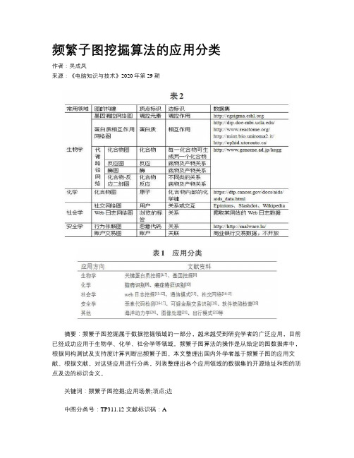
频繁子图挖掘算法的应用分类作者：吴成凤来源：《电脑知识与技术》2020年第29期摘要：频繁子图挖掘属于数据挖掘领域的一部分，越来越受到研究学者的广泛应用，目前已经成功应用于生物学、化学、社会学等领域。

频繁子图算法的操作是从给定的图数据库中，根据同构测试及支持度计算判断出频繁子图。

本文整理出国内外学者基于频繁子图的应用文献。

根据文献，对这些应用进行分类，列表整理出各个应用领域的数据集的开源地址和图的顶点及边的标识含义。

关键词：频繁子图挖掘;应用场景;顶点;边中图分类号：TP311.12 文献标识码：A文章编号：1009-3044（2020）29-0040-021 引言在数据挖掘的领域中，频繁子图挖掘算法越来越受到国内外研究学者的关注。

频繁子图将各种数据处理成顶点到顶点的逻辑关系的表示，在该模型[1]中，顶点和对应的边关系可以具有与它们相关联的标签，这些标签不是唯一的。

使用这样的图表示，频繁模式的问题变成了在整个图上寻求频繁出现子图的问题，运用频繁子图算法挖掘其潜在的价值。

频繁子图挖掘算法即在给定的图中根据设定的支持度阈值，寻找出同构子图大于等于给定支持度阈值的子图。

频繁子图算法的发展历经二十年，基于频繁子图的应用也越来越广泛。

2 运用场景在由顶点和边构成的图中，顶点有其分类的标识，边亦有其分类的标识，我们需要在给定的图数据库中寻找出顶点标识和标识对应一致的子图，计算出支持度，若一旦支持度超过给定的阈值，便输出其子图，其子图便是一个频繁子图。

Lin W[2]等人认为频繁子图挖掘问题分为两个方面：在一个大图的不同区域挖掘子图适用于社交网络分析等领域;在大规模图集中挖掘子图适用于生物信息学和计算药理学等领域。

图集上的挖掘是指在多张图的图数据库中挖掘这些图中共现的子图。

在一张大图上的挖掘则是在一张图上挖掘图内出现的子图。

基于图事务集合的频繁子图挖掘算法与基于单个大图的频繁子图挖掘算法不同，在计算候选子图支持度的时候，基于图事务集合的频繁子图挖掘算法只需要计算候选子图与图事务集合中满足子图同构的小图的个数，而基于单个大图的频繁子图挖掘算法需要在这个大图中找出候选子图所有的同构的子图，计算用同构的子图的候选子图支持度[3]。

一种存储复杂多边形包含关系的四叉树索引
四叉树是一种用来划分二维空间的树状数据结构，可以用来存储和检索包含关系。

在
存储复杂多边形的包含关系时，可以利用四叉树索引来提高存储和查询的效率。

四叉树是一种将空间划分为四个象限的树结构。

每个节点有四个子节点，每个子节点
对应一个象限。

树的根节点代表整个二维空间，然后通过递归将空间划分为四分之一，并
一直划分下去，直到达到一个最小单位。

在存储复杂多边形的包含关系时，可以根据多边形的边界框来划分空间并构建四叉树。

边界框是一个矩形，包含了多边形的最小外接矩形。

首先找到整个多边形集合的边界框，
然后将边界框划分为四个象限，分别找到每个象限内包含的多边形，并用四叉树的节点来
表示这些多边形。

然后对每个节点再进行递归划分，直到每个叶子节点只包含一个多边
形。

在查询复杂多边形的包含关系时，可以通过四叉树索引来提高查询效率。

首先找到查
询多边形的边界框，然后判断边界框与四叉树节点的相交关系。

如果边界框与节点不相交，则可以跳过该节点及其子节点，不需要进一步的遍历。

如果边界框与节点相交，则需要继
续对子节点进行检查，直到达到叶子节点。

最后可以检查叶子节点内的多边形是否与查询
多边形相交，从而确定是否包含。

四叉树索引可以大大减少查询的次数，提高查询的效率。

因为每个节点都代表了一个
空间区域，所以通过判断边界框的相交关系可以快速排除不相关的节点。

四叉树索引对于
复杂多边形的包含关系的查询也非常高效，因为每个叶子节点只包含一个多边形，不需要
进行进一步的判断。

基于梯度选择的轻量化差分隐私保护联邦学习王周生;杨庚;戴华【期刊名称】《计算机科学》【年(卷),期】2024(51)1【摘要】为了应对机器学习过程中可能出现的用户隐私问题,联邦学习作为首个无需用户上传真实数据、仅上传模型更新的协作式在线学习解决方案,已经受到人们的广泛关注与研究。

然而,它要求用户在本地训练且上传的模型更新中仍可能包含敏感信息,从而带来了新的隐私保护问题。

与此同时,必须在用户本地进行完整训练的特点也使得联邦学习过程中的运算与通信开销问题成为一项挑战,亟需人们建立一种轻量化的联邦学习架构体系。

出于进一步的隐私需求考虑,文中使用了带有差分隐私机制的联邦学习框架。

另外,首次提出了基于Fisher信息矩阵的Dropout 机制——FisherDropout,用于对联邦学习过程中在客户端训练产生梯度更新的每个维度进行优化选择,从而极大地节约运算成本、通信成本以及隐私预算,建立了一种兼具隐私性与轻量化优势的联邦学习框架。

在真实世界数据集上的大量实验验证了该方案的有效性。

实验结果表明,相比其他联邦学习框架,FisherDropout机制在最好的情况下可以节约76.8%~83.6%的通信开销以及23.0%~26.2%的运算开销,在差分隐私保护中隐私性与可用性的均衡方面同样具有突出优势。

【总页数】10页(P345-354)【作者】王周生;杨庚;戴华【作者单位】南京邮电大学计算机学院;江苏省大数据安全与智能处理重点实验室【正文语种】中文【中图分类】TP309【相关文献】1.基于差分隐私的联邦学习数据隐私安全技术2.面向联邦学习的学习率裁剪梯度优化隐私保护方案3.基于差分隐私保护知识迁移的联邦学习方法4.基于本地差分隐私的联邦学习隐私保护方法5.结合联邦学习和增强学习的车联网数据差分隐私保护因版权原因，仅展示原文概要，查看原文内容请购买。

人工智能中的蒙特卡罗树搜索算法随着人工智能的不断发展，各种算法也不断涌现。

其中，蒙特卡罗树搜索算法是一种在游戏和决策中广泛应用的算法。

本文将会介绍蒙特卡罗树搜索算法的基本原理和应用场景。

1. 蒙特卡罗树搜索算法的基本原理蒙特卡罗树搜索算法是一种基于蒙特卡罗模拟的搜索算法，能够在感知时间内找到每个可能的行动，以及每个行动的可能结果。

该算法依赖于随机化计算，通过大量模拟实验获取每个决策的成功率及其期望回报。

蒙特卡罗树搜索算法是通过创建搜索树，不断拓展每个节点来实现的。

该算法的基本步骤如下：首先，我们需要构建搜索树。

搜索树的根节点表示我们的当前状态，每个子节点表示我们执行某一行为后的状态。

其次，我们需要进行蒙特卡罗模拟。

在每个节点处，我们需要使用随机数生成器模拟一些行动，通过大量模拟实验获取每个决策的成功率及其期望回报。

随后，我们要从当前的节点开始扩展搜索，以生成搜索树的枝条。

我们在树叶处运行模拟，所得的奖励值将传递回已经访问的各级节点。

最后，根据得到的每个子节点期望价值，我们可以选择选择最优的子节点行为。

当我们选择子节点时，需要计算每个子节点的平均值，并考虑平均值约束的置信度，以便更好地选择下一个子节点。

2. 蒙特卡罗树搜索算法的应用场景蒙特卡罗树搜索算法具有广泛的应用场景。

最常见的应用之一是在游戏中，特别是在棋类游戏中。

例如，中国象棋和围棋都可以通过蒙特卡罗树搜索算法进行智能对弈。

此外，在决策问题中也可以采用蒙特卡罗树搜索算法。

例如，在互联网广告中，需要确定哪些广告应该在哪些位置上展示，以最大化投资回报。

蒙特卡罗树搜索算法可以通过生成树来搜索各种广告组合，以找到最佳结果。

总之，蒙特卡罗树搜索算法已经成为了人工智能中的重要算法之一。

它的基本原理是通过随机化计算，获取每个决策的成功率及其期望回报，并通过搜索树在时间感知的条件下找到每个可能的行动以及每个行动的可能结果。

在游戏、决策等领域中广泛应用。

A review on time series data miningTak-chung FuDepartment of Computing,Hong Kong Polytechnic University,Hunghom,Kowloon,Hong Konga r t i c l e i n f oArticle history:Received19February2008Received in revised form14March2010Accepted4September2010Keywords:Time series data miningRepresentationSimilarity measureSegmentationVisualizationa b s t r a c tTime series is an important class of temporal data objects and it can be easily obtained from scientificandfinancial applications.A time series is a collection of observations made chronologically.The natureof time series data includes:large in data size,high dimensionality and necessary to updatecontinuously.Moreover time series data,which is characterized by its numerical and continuousnature,is always considered as a whole instead of individual numericalfield.The increasing use of timeseries data has initiated a great deal of research and development attempts in thefield of data mining.The abundant research on time series data mining in the last decade could hamper the entry ofinterested researchers,due to its complexity.In this paper,a comprehensive revision on the existingtime series data mining researchis given.They are generally categorized into representation andindexing,similarity measure,segmentation,visualization and mining.Moreover state-of-the-artresearch issues are also highlighted.The primary objective of this paper is to serve as a glossary forinterested researchers to have an overall picture on the current time series data mining developmentand identify their potential research direction to further investigation.&2010Elsevier Ltd.All rights reserved.1.IntroductionRecently,the increasing use of temporal data,in particulartime series data,has initiated various research and developmentattempts in thefield of data mining.Time series is an importantclass of temporal data objects,and it can be easily obtained fromscientific andfinancial applications(e.g.electrocardiogram(ECG),daily temperature,weekly sales totals,and prices of mutual fundsand stocks).A time series is a collection of observations madechronologically.The nature of time series data includes:large indata size,high dimensionality and update continuously.Moreovertime series data,which is characterized by its numerical andcontinuous nature,is always considered as a whole instead ofindividual numericalfield.Therefore,unlike traditional databaseswhere similarity search is exact match based,similarity search intime series data is typically carried out in an approximatemanner.There are various kinds of time series data related research,forexample,finding similar time series(Agrawal et al.,1993a;Berndtand Clifford,1996;Chan and Fu,1999),subsequence searching intime series(Faloutsos et al.,1994),dimensionality reduction(Keogh,1997b;Keogh et al.,2000)and segmentation(Abonyiet al.,2005).Those researches have been studied in considerabledetail by both database and pattern recognition communities fordifferent domains of time series data(Keogh and Kasetty,2002).In the context of time series data mining,the fundamentalproblem is how to represent the time series data.One of thecommon approaches is transforming the time series to anotherdomain for dimensionality reduction followed by an indexingmechanism.Moreover similarity measure between time series ortime series subsequences and segmentation are two core tasksfor various time series mining tasks.Based on the time seriesrepresentation,different mining tasks can be found in theliterature and they can be roughly classified into fourfields:pattern discovery and clustering,classification,rule discovery andsummarization.Some of the research concentrates on one of thesefields,while the others may focus on more than one of the aboveprocesses.In this paper,a comprehensive review on the existingtime series data mining research is given.Three state-of-the-arttime series data mining issues,streaming,multi-attribute timeseries data and privacy are also briefly introduced.The remaining part of this paper is organized as follows:Section2contains a discussion of time series representation andindexing.The concept of similarity measure,which includes bothwhole time series and subsequence matching,based on the rawtime series data or the transformed domain will be reviewed inSection3.The research work on time series segmentation andvisualization will be discussed in Sections4and5,respectively.InSection6,vary time series data mining tasks and recent timeseries data mining directions will be reviewed,whereas theconclusion will be made in Section7.2.Time series representation and indexingOne of the major reasons for time series representation is toreduce the dimension(i.e.the number of data point)of theContents lists available at ScienceDirectjournal homepage:/locate/engappaiEngineering Applications of Artificial Intelligence0952-1976/$-see front matter&2010Elsevier Ltd.All rights reserved.doi:10.1016/j.engappai.2010.09.007E-mail addresses:cstcfu@.hk,cstcfu@Engineering Applications of Artificial Intelligence24(2011)164–181original data.The simplest method perhaps is sampling(Astrom, 1969).In this method,a rate of m/n is used,where m is the length of a time series P and n is the dimension after dimensionality reduction(Fig.1).However,the sampling method has the drawback of distorting the shape of sampled/compressed time series,if the sampling rate is too low.An enhanced method is to use the average(mean)value of each segment to represent the corresponding set of data points. Again,with time series P¼ðp1,...,p mÞand n is the dimension after dimensionality reduction,the‘‘compressed’’time series ^P¼ð^p1,...,^p nÞcan be obtained by^p k ¼1k kX e ki¼s kp ið1Þwhere s k and e k denote the starting and ending data points of the k th segment in the time series P,respectively(Fig.2).That is, using the segmented means to represent the time series(Yi and Faloutsos,2000).This method is also called piecewise aggregate approximation(PAA)by Keogh et al.(2000).1Keogh et al.(2001a) propose an extended version called an adaptive piecewise constant approximation(APCA),in which the length of each segment is notfixed,but adaptive to the shape of the series.A signature technique is proposed by Faloutsos et al.(1997)with similar ideas.Besides using the mean to represent each segment, other methods are proposed.For example,Lee et al.(2003) propose to use the segmented sum of variation(SSV)to represent each segment of the time series.Furthermore,a bit level approximation is proposed by Ratanamahatana et al.(2005)and Bagnall et al.(2006),which uses a bit to represent each data point.To reduce the dimension of time series data,another approach is to approximate a time series with straight lines.Two major categories are involved.Thefirst one is linear interpolation.A common method is using piecewise linear representation(PLR)2 (Keogh,1997b;Keogh and Smyth,1997;Smyth and Keogh,1997). The approximating line for the subsequence P(p i,y,p j)is simply the line connecting the data points p i and p j.It tends to closely align the endpoint of consecutive segments,giving the piecewise approximation with connected lines.PLR is a bottom-up algo-rithm.It begins with creating afine approximation of the time series,so that m/2segments are used to approximate the m length time series and iteratively merges the lowest cost pair of segments,until it meets the required number of segment.When the pair of adjacent segments S i and S i+1are merged,the cost of merging the new segment with its right neighbor and the cost of merging the S i+1segment with its new larger neighbor is calculated.Ge(1998)extends PLR to hierarchical structure. Furthermore,Keogh and Pazzani enhance PLR by considering weights of the segments(Keogh and Pazzani,1998)and relevance feedback from the user(Keogh and Pazzani,1999).The second approach is linear regression,which represents the subsequences with the bestfitting lines(Shatkay and Zdonik,1996).Furthermore,reducing the dimension by preserving the salient points is a promising method.These points are called as perceptually important points(PIP).The PIP identification process isfirst introduced by Chung et al.(2001)and used for pattern matching of technical(analysis)patterns infinancial applications. With the time series P,there are n data points:P1,P2y,P n.All the data points in P can be reordered by its importance by going through the PIP identification process.Thefirst data point P1and the last data point P n in the time series are thefirst and two PIPs, respectively.The next PIP that is found will be the point in P with maximum distance to thefirst two PIPs.The fourth PIP that is found will be the point in P with maximum vertical distance to the line joining its two adjacent PIPs,either in between thefirst and second PIPs or in between the second and the last PIPs.The PIP location process continues until all the points in P are attached to a reordered list L or the required number of PIPs is reached(i.e. reduced to the required dimension).Seven PIPs are identified in from the sample time series in Fig.3.Detailed treatment can be found in Fu et al.(2008c).The idea is similar to a technique proposed about30years ago for reducing the number of points required to represent a line by Douglas and Peucker(1973)(see also Hershberger and Snoeyink, 1992).Perng et al.(2000)use a landmark model to identify the important points in the time series for similarity measure.Man and Wong(2001)propose a lattice structure to represent the identified peaks and troughs(called control points)in the time series.Pratt and Fink(2002)and Fink et al.(2003)define extrema as minima and maxima in a time series and compress thetime Fig.1.Time series dimensionality reduction by sampling.The time series on the left is sampled regularly(denoted by dotted lines)and displayed on the right with a largedistortion.Fig.2.Time series dimensionality reduction by PAA.The horizontal dotted lines show the mean of each segment.1This method is called piecewise constant approximation originally(Keoghand Pazzani,2000a).2It is also called piecewise linear approximation(PLA).Tak-chung Fu/Engineering Applications of Artificial Intelligence24(2011)164–181165series by selecting only certain important extrema and dropping the other points.The idea is to discard minor fluctuations and keep major minima and maxima.The compression is controlled by the compression ratio with parameter R ,which is always greater than one;an increase of R leads to the selection of fewer points.That is,given indices i and j ,where i r x r j ,a point p x of a series P is an important minimum if p x is the minimum among p i ,y ,p j ,and p i /p x Z R and p j /p x Z R .Similarly,p x is an important maximum if p x is the maximum among p i ,y ,p j and p x /p i Z R and p x /p j Z R .This algorithm takes linear time and constant memory.It outputs the values and indices of all important points,as well as the first and last point of the series.This algorithm can also process new points as they arrive,without storing the original series.It identifies important points based on local information of each segment (subsequence)of time series.Recently,a critical point model (CPM)(Bao,2008)and a high-level representation based on a sequence of critical points (Bao and Yang,2008)are proposed for financial data analysis.On the other hand,special points are introduced to restrict the error on PLR (Jia et al.,2008).Key points are suggested to represent time series in (Leng et al.,2009)for an anomaly detection.Another common family of time series representation approaches converts the numeric time series to symbolic form.That is,first discretizing the time series into segments,then converting each segment into a symbol (Yang and Zhao,1998;Yang et al.,1999;Motoyoshi et al.,2002;Aref et al.,2004).Lin et al.(2003;2007)propose a method called symbolic aggregate approximation (SAX)to convert the result from PAA to symbol string.The distribution space (y -axis)is divided into equiprobable regions.Each region is represented by a symbol and each segment can then be mapped into a symbol corresponding to the region inwhich it resides.The transformed time series ^Pusing PAA is finally converted to a symbol string SS (s 1,y ,s W ).In between,two parameters must be specified for the conversion.They are the length of subsequence w and alphabet size A (number of symbols used).Besides using the means of the segments to build the alphabets,another method uses the volatility change to build the alphabets.Jonsson and Badal (1997)use the ‘‘Shape Description Alphabet (SDA)’’.Example symbols like highly increasing transi-tion,stable transition,and slightly decreasing transition are adopted.Qu et al.(1998)use gradient alphabets like upward,flat and download as symbols.Huang and Yu (1999)suggest transforming the time series to symbol string,using change ratio between contiguous data points.Megalooikonomou et al.(2004)propose to represent each segment by a codeword from a codebook of key-sequences.This work has extended to multi-resolution consideration (Megalooi-konomou et al.,2005).Morchen and Ultsch (2005)propose an unsupervised discretization process based on quality score and persisting states.Instead of ignoring the temporal order of values like many other methods,the Persist algorithm incorporates temporal information.Furthermore,subsequence clustering is a common method to generate the symbols (Das et al.,1998;Li et al.,2000a;Hugueney and Meunier,2001;Hebrail and Hugueney,2001).A multiple abstraction level mining (MALM)approach is proposed by Li et al.(1998),which is based on the symbolic form of the time series.The symbols in this paper are determined by clustering the features of each segment,such as regression coefficients,mean square error and higher order statistics based on the histogram of the regression residuals.Most of the methods described so far are representing time series in time domain directly.Representing time series in the transformation domain is another large family of approaches.One of the popular transformation techniques in time series data mining is the discrete Fourier transforms (DFT),since first being proposed for use in this context by Agrawal et al.(1993a).Rafiei and Mendelzon (2000)develop similarity-based queries,using DFT.Janacek et al.(2005)propose to use likelihood ratio statistics to test the hypothesis of difference between series instead of an Euclidean distance in the transformed domain.Recent research uses wavelet transform to represent time series (Struzik and Siebes,1998).In between,the discrete wavelet transform (DWT)has been found to be effective in replacing DFT (Chan and Fu,1999)and the Haar transform is always selected (Struzik and Siebes,1999;Wang and Wang,2000).The Haar transform is a series of averaging and differencing operations on a time series (Chan and Fu,1999).The average and difference between every two adjacent data points are computed.For example,given a time series P ¼(1,3,7,5),dimension of 4data points is the full resolution (i.e.original time series);in dimension of two coefficients,the averages are (26)with the coefficients (À11)and in dimension of 1coefficient,the average is 4with coefficient (À2).A multi-level representation of the wavelet transform is proposed by Shahabi et al.(2000).Popivanov and Miller (2002)show that a large class of wavelet transformations can be used for time series representation.Dasha et al.(2007)compare different wavelet feature vectors.On the other hand,comparison between DFT and DWT can be found in Wu et al.(2000b)and Morchen (2003)and a combination use of Fourier and wavelet transforms are presented in Kawagoe and Ueda (2002).An ensemble-index,is proposed by Keogh et al.(2001b)and Vlachos et al.(2006),which ensembles two or more representations for indexing.Principal component analysis (PCA)is a popular multivariate technique used for developing multivariate statistical process monitoring methods (Yang and Shahabi,2005b;Yoon et al.,2005)and it is applied to analyze financial time series by Lesch et al.(1999).In most of the related works,PCA is used to eliminate the less significant components or sensors and reduce the data representation only to the most significant ones and to plot the data in two dimensions.The PCA model defines linear hyperplane,it can be considered as the multivariate extension of the PLR.PCA maps the multivariate data into a lower dimensional space,which is useful in the analysis and visualization of correlated high-dimensional data.Singular value decomposition (SVD)(Korn et al.,1997)is another transformation-based approach.Other time series representation methods include modeling time series using hidden markov models (HMMs)(Azzouzi and Nabney,1998)and a compression technique for multiple stream is proposed by Deligiannakis et al.(2004).It is based onbaseFig.3.Time series compression by data point importance.The time series on the left is represented by seven PIPs on the right.Tak-chung Fu /Engineering Applications of Artificial Intelligence 24(2011)164–181166signal,which encodes piecewise linear correlations among the collected data values.In addition,a recent biased dimension reduction technique is proposed by Zhao and Zhang(2006)and Zhao et al.(2006).Moreover many of the representation schemes described above are incorporated with different indexing methods.A common approach is adopted to an existing multidimensional indexing structure(e.g.R-tree proposed by Guttman(1984))for the representation.Agrawal et al.(1993a)propose an F-index, which adopts the R*-tree(Beckmann et al.,1990)to index thefirst few DFT coefficients.An ST-index is further proposed by (Faloutsos et al.(1994),which extends the previous work for subsequence handling.Agrawal et al.(1995a)adopt both the R*-and R+-tree(Sellis et al.,1987)as the indexing structures.A multi-level distance based index structure is proposed(Yang and Shahabi,2005a),which for indexing time series represented by PCA.Vlachos et al.(2005a)propose a Multi-Metric(MM)tree, which is a hybrid indexing structure on Euclidean and periodic spaces.Minimum bounding rectangle(MBR)is also a common technique for time series indexing(Chu and Wong,1999;Vlachos et al.,2003).An MBR is adopted in(Rafiei,1999)which an MT-index is developed based on the Fourier transform and in(Kahveci and Singh,2004)which a multi-resolution index is proposed based on the wavelet transform.Chen et al.(2007a)propose an indexing mechanism for PLR representation.On the other hand, Kim et al.(1996)propose an index structure called TIP-index (TIme series Pattern index)for manipulating time series pattern databases.The TIP-index is developed by improving the extended multidimensional dynamic indexfile(EMDF)(Kim et al.,1994). An iSAX(Shieh and Keogh,2009)is proposed to index massive time series,which is developed based on an SAX.A multi-resolution indexing structure is proposed by Li et al.(2004),which can be adapted to different representations.To sum up,for a given index structure,the efficiency of indexing depends only on the precision of the approximation in the reduced dimensionality space.However in choosing a dimensionality reduction technique,we cannot simply choose an arbitrary compression algorithm.It requires a technique that produces an indexable representation.For example,many time series can be efficiently compressed by delta encoding,but this representation does not lend itself to indexing.In contrast,SVD, DFT,DWT and PAA all lend themselves naturally to indexing,with each eigenwave,Fourier coefficient,wavelet coefficient or aggregate segment map onto one dimension of an index tree. Post-processing is then performed by computing the actual distance between sequences in the time domain and discarding any false matches.3.Similarity measureSimilarity measure is of fundamental importance for a variety of time series analysis and data mining tasks.Most of the representation approaches discussed in Section2also propose the similarity measure method on the transformed representation scheme.In traditional databases,similarity measure is exact match based.However in time series data,which is characterized by its numerical and continuous nature,similarity measure is typically carried out in an approximate manner.Consider the stock time series,one may expect having queries like: Query1:find all stocks which behave‘‘similar’’to stock A.Query2:find all‘‘head and shoulders’’patterns last for a month in the closing prices of all high-tech stocks.The query results are expected to provide useful information for different stock analysis activities.Queries like Query2in fact is tightly coupled with the patterns frequently used in technical analysis, e.g.double top/bottom,ascending triangle,flag and rounded top/bottom.In time series domain,devising an appropriate similarity function is by no means trivial.There are essentially two ways the data that might be organized and processed(Agrawal et al., 1993a).In whole sequence matching,the whole length of all time series is considered during the similarity search.It requires comparing the query sequence to each candidate series by evaluating the distance function and keeping track of the sequence with the smallest distance.In subsequence matching, where a query sequence Q and a longer sequence P are given,the task is tofind the subsequences in P,which matches Q. Subsequence matching requires that the query sequence Q be placed at every possible offset within the longer sequence P.With respect to Query1and Query2above,they can be considered as a whole sequence matching and a subsequence matching,respec-tively.Gavrilov et al.(2000)study the usefulness of different similarity measures for clustering similar stock time series.3.1.Whole sequence matchingTo measure the similarity/dissimilarity between two time series,the most popular approach is to evaluate the Euclidean distance on the transformed representation like the DFT coeffi-cients(Agrawal et al.,1993a)and the DWT coefficients(Chan and Fu,1999).Although most of these approaches guarantee that a lower bound of the Euclidean distance to the original data, Euclidean distance is not always being the suitable distance function in specified domains(Keogh,1997a;Perng et al.,2000; Megalooikonomou et al.,2005).For example,stock time series has its own characteristics over other time series data(e.g.data from scientific areas like ECG),in which the salient points are important.Besides Euclidean-based distance measures,other distance measures can easily be found in the literature.A constraint-based similarity query is proposed by Goldin and Kanellakis(1995), which extended the work of(Agrawal et al.,1993a).Das et al. (1997)apply computational geometry methods for similarity measure.Bozkaya et al.(1997)use a modified edit distance function for time series matching and retrieval.Chu et al.(1998) propose to measure the distance based on the slopes of the segments for handling amplitude and time scaling problems.A projection algorithm is proposed by Lam and Wong(1998).A pattern recognition method is proposed by Morrill(1998),which is based on the building blocks of the primitives of the time series. Ruspini and Zwir(1999)devote an automated identification of significant qualitative features of complex objects.They propose the process of discovery and representation of interesting relations between those features,the generation of structured indexes and textual annotations describing features and their relations.The discovery of knowledge by an analysis of collections of qualitative descriptions is then achieved.They focus on methods for the succinct description of interesting features lying in an effective frontier.Generalized clustering is used for extracting features,which interest domain experts.The general-ized Markov models are adopted for waveform matching in Ge and Smyth(2000).A content-based query-by-example retrieval model called FALCON is proposed by Wu et al.(2000a),which incorporates a feedback mechanism.Indeed,one of the most popular andfield-tested similarity measures is called the‘‘time warping’’distance measure.Based on the dynamic time warping(DTW)technique,the proposed method in(Berndt and Clifford,1994)predefines some patterns to serve as templates for the purpose of pattern detection.To align two time series,P and Q,using DTW,an n-by-m matrix M isfirstTak-chung Fu/Engineering Applications of Artificial Intelligence24(2011)164–181167constructed.The(i th,j th)element of the matrix,m ij,contains the distance d(q i,p j)between the two points q i and p j and an Euclidean distance is typically used,i.e.d(q i,p j)¼(q iÀp j)2.It corresponds to the alignment between the points q i and p j.A warping path,W,is a contiguous set of matrix elements that defines a mapping between Q and P.Its k th element is defined as w k¼(i k,j k)andW¼w1,w2,...,w k,...,w Kð2Þwhere maxðm,nÞr K o mþnÀ1.The warping path is typically subjected to the following constraints.They are boundary conditions,continuity and mono-tonicity.Boundary conditions are w1¼(1,1)and w K¼(m,n).This requires the warping path to start andfinish diagonally.Next constraint is continuity.Given w k¼(a,b),then w kÀ1¼(a0,b0), where aÀa u r1and bÀb u r1.This restricts the allowable steps in the warping path being the adjacent cells,including the diagonally adjacent cell.Also,the constraints aÀa uZ0and bÀb uZ0force the points in W to be monotonically spaced in time.There is an exponential number of warping paths satisfying the above conditions.However,only the path that minimizes the warping cost is of interest.This path can be efficiently found by using dynamic programming(Berndt and Clifford,1996)to evaluate the following recurrence equation that defines the cumulative distance gði,jÞas the distance dði,jÞfound in the current cell and the minimum of the cumulative distances of the adjacent elements,i.e.gði,jÞ¼dðq i,p jÞþmin f gðiÀ1,jÀ1Þ,gðiÀ1,jÞ,gði,jÀ1Þgð3ÞA warping path,W,such that‘‘distance’’between them is minimized,can be calculated by a simple methodDTWðQ,PÞ¼minWX Kk¼1dðw kÞ"#ð4Þwhere dðw kÞcan be defined asdðw kÞ¼dðq ik ,p ikÞ¼ðq ikÀp ikÞ2ð5ÞDetailed treatment can be found in Kruskall and Liberman (1983).As DTW is computationally expensive,different methods are proposed to speedup the DTW matching process.Different constraint(banding)methods,which control the subset of matrix that the warping path is allowed to visit,are reviewed in Ratanamahatana and Keogh(2004).Yi et al.(1998)introduce a technique for an approximate indexing of DTW that utilizes a FastMap technique,whichfilters the non-qualifying series.Kim et al.(2001)propose an indexing approach under DTW similarity measure.Keogh and Pazzani(2000b)introduce a modification of DTW,which integrates with PAA and operates on a higher level abstraction of the time series.An exact indexing approach,which is based on representing the time series by PAA for DTW similarity measure is further proposed by Keogh(2002).An iterative deepening dynamic time warping(IDDTW)is suggested by Chu et al.(2002),which is based on a probabilistic model of the approximate errors for all levels of approximation prior to the query process.Chan et al.(2003)propose afiltering process based on the Haar wavelet transformation from low resolution approx-imation of the real-time warping distance.Shou et al.(2005)use an APCA approximation to compute the lower bounds for DTW distance.They improve the global bound proposed by Kim et al. (2001),which can be used to index the segments and propose a multi-step query processing technique.A FastDTW is proposed by Salvador and Chan(2004).This method uses a multi-level approach that recursively projects a solution from a coarse resolution and refines the projected solution.Similarly,a fast DTW search method,an FTW is proposed by Sakurai et al.(2005) for efficiently pruning a significant number of search candidates. Ratanamahatana and Keogh(2005)clarified some points about DTW where are related to lower bound and speed.Euachongprasit and Ratanamahatana(2008)also focus on this problem.A sequentially indexed structure(SIS)is proposed by Ruengron-ghirunya et al.(2009)to balance the tradeoff between indexing efficiency and I/O cost during DTW similarity measure.A lower bounding function for group of time series,LBG,is adopted.On the other hand,Keogh and Pazzani(2001)point out the potential problems of DTW that it can lead to unintuitive alignments,where a single point on one time series maps onto a large subsection of another time series.Also,DTW may fail to find obvious and natural alignments in two time series,because of a single feature(i.e.peak,valley,inflection point,plateau,etc.). One of the causes is due to the great difference between the lengths of the comparing series.Therefore,besides improving the performance of DTW,methods are also proposed to improve an accuracy of DTW.Keogh and Pazzani(2001)propose a modifica-tion of DTW that considers the higher level feature of shape for better alignment.Ratanamahatana and Keogh(2004)propose to learn arbitrary constraints on the warping path.Regression time warping(RTW)is proposed by Lei and Govindaraju(2004)to address the challenges of shifting,scaling,robustness and tecki et al.(2005)propose a method called the minimal variance matching(MVM)for elastic matching.It determines a subsequence of the time series that best matches a query series byfinding the cheapest path in a directed acyclic graph.A segment-wise time warping distance(STW)is proposed by Zhou and Wong(2005)for time scaling search.Fu et al.(2008a) propose a scaled and warped matching(SWM)approach for handling both DTW and uniform scaling simultaneously.Different customized DTW techniques are applied to thefield of music research for query by humming(Zhu and Shasha,2003;Arentz et al.,2005).Focusing on similar problems as DTW,the Longest Common Subsequence(LCSS)model(Vlachos et al.,2002)is proposed.The LCSS is a variation of the edit distance and the basic idea is to match two sequences by allowing them to stretch,without rearranging the sequence of the elements,but allowing some elements to be unmatched.One of the important advantages of an LCSS over DTW is the consideration on the outliers.Chen et al.(2005a)further introduce a distance function based on an edit distance on real sequence(EDR),which is robust against the data imperfection.Morse and Patel(2007)propose a Fast Time Series Evaluation(FTSE)method which can be used to evaluate the threshold value of these kinds of techniques in a faster way.Threshold-based distance functions are proposed by ABfalg et al. (2006).The proposed function considers intervals,during which the time series exceeds a certain threshold for comparing time series rather than using the exact time series values.A T-Time application is developed(ABfalg et al.,2008)to demonstrate the usage of it.Fu et al.(2007)further suggest to introduce rules to govern the pattern matching process,if a priori knowledge exists in the given domain.A parameter-light distance measure method based on Kolmo-gorov complexity theory is suggested in Keogh et al.(2007b). Compression-based dissimilarity measure(CDM)3is adopted in this paper.Chen et al.(2005b)present a histogram-based representation for similarity measure.Similarly,a histogram-based similarity measure,bag-of-patterns(BOP)is proposed by Lin and Li(2009).The frequency of occurrences of each pattern in 3CDM is proposed by Keogh et al.(2004),which is used to compare the co-compressibility between data sets.Tak-chung Fu/Engineering Applications of Artificial Intelligence24(2011)164–181 168。