《金融工程》案例解析(英文版)
- 格式:pptx
- 大小:646.31 KB
- 文档页数:27

AbstractPurpose –The purpose of this paper is to provide a general discussion of how techniques from financial engineering can be used to investigate the economic costs of farm programs and to aid in the design of new financial products to implement margin protection for dairy farmers. Specifically the paper investigates the Milk Income Loss Contract (MILC) and the Dairy Margin Protection (DMP) program. In addition the paper introduces the concept of the Milk to Corn Price ratio to protect margins.Design/methodology/approach –The paper introduces and reviews the tools of financial engineering. These include the stochastic calculus and Itoˆ’s Lemma. The empirical tool is Monte Carlosimulations. The approach is part pedagogy and part practice.Findings –In this paper the authors illustrate how financial engineering can be used to price complex price stabilization formula in the USA and to illustrate its use in the design of new products. Practical implications –In this paper the authors illustrate how financial engineering can be used to price complex price stabilization formula in the USA and to illustrate its use in the design of new products.Social implications–Farm programs designed to protect dairy farmers margins are designed in a seemingly ad hoc fashion. Assessments of programs such as MILC or DMP are conducted on an ex-post basis using historical data. The financial engineering approach presented in this paper provides the means to add significant depth to the assessment of such programs which can be used in conjunction with Monte Carlo simulation to identify alternative model structures before they are written into law.Originality/value –This paper builds upon an existing literature. Its originality is in the application of financial engineering techniques to farm dairy policy.Keywords :Dairy policy, DMP, Financial Engineering, Itoˆ’s lemma, MILC, Milk to corn ratio Agricultural policy in the USA and elsewhere has from time to time established programs that in one form or another have been structured around the randomness of prices with the objective of providing some form of stabilization. These have included loan rates and target prices under the Commodity Credit Corporation until 2002 and currently revolving around flex payments, direct and countercyclical payments, SURE (the Supplemental Revenue Assistance Program), ACRE (Average Crop Revenue Election) and for dairy the Milk Income Loss Contract (MILC) in the 2008 Farm Bill (Bekkerman et al, 2012). In addition to these, new programs have evolved on a revenue basis with insurance indemnities paid on the joint outcomes of crop yield and market prices. Indeed, it seems that any new Farm Bill has some evolutionary or revolutionary stabilization program as part of its text, and sometimes in a rather convoluted and seemingly ad hoc form. For example, a host of volumetric or revenue-based programs are proposed in the 2013 Farm Bill including ARC (Agricultural Risk Coverage), STAX (the Stacked Income Protection Plan), RLC (Revenue Loss Coverage) and SCO (The Supplemental Coverage Option) (Paulson et al., 2013; Barut and Collins, 2014).Since the 1970s there has been a general interest in determining the value of a particular program both in terms of welfare to farmers and public expenditure to the tax payers (Marcus and Modest, 1986; Brinch and Stokes, 2001; Hertzler, 1991; Pederson and Zhou, 2009; Richards and Manfredo, 2003; Stokes and Nayda, 2003; Stokes et al., 1997; Tirupattur et al., 1997; Turvey et al., 1988; Turvey, 1992; Turvey and Stokes, 2008; Yin and Turvey, 2003). But while this interest is alwaysthere, the actual practice of determining program value has been limited in application. The traditional approach to valuing agricultural policy programs has relied heavily on demand and supply side interactions to generate price changes. However, in practice, price dynamics of both inputs and outputs are subject to significant variation that is persistent, volatile and unexplained by equilibrium models. Financial engineering uses stochastic calculus to directly model price dynamics and the underlying risks embedded in the farm problem.In this paper we explore financial engineering as a mechanism for understanding the farm problem in a number of contexts. First we introduce the idea of financial engineering through a primer on the stochastic calculus or Itoˆ’s Lemma (Itoˆ, 1942a, b, 1944a, b, 1951a, b; Jarrow and Protter, 2004; McKean 2007). Then we show how contingent claims policies such as MILC and Dairy Margin Protection (DMP) with non-linear payoffs to farmers can be priced or valued using financial engineering techniques similar to the pricing of conventional options in a Black and Scholes (1973) framework. We also illustrate how new risk management products can be financially engineered. In particular, we apply financial engineering techniques to the milk to corn price ratio and provide some preliminary evidence on the effectiveness of the new risk management product in hedging milk revenue margins.Dairy producers confront various sources of risk. Among those, the uncertainty associated with the future cash price of a commodity is known as price risk. Theincrease in the price volatility of milk, corn and soybean in recent years[1] poses an increasing threat to the business survival of dairy producers. In New York State all-milk prices have not increased much for the past 15 years[2] while corn and soybean prices have soared since 2006. While the rising feed costs may be temporary, if dairy farmers in New York are inadequately hedged against this risk, shrinking profit margins may lead them to the brink of bankruptcy. Consequently, dairy farm profits are not only affected by the price risk from the milk price received, but also by the volatility in input prices. Dairy feed, which mainly consists of corn, hay and soybean, is one of the most important inputs for dairy producers. As a non-storable commodity, there could be large swings in milk prices in reaction to changes in market fundamentals. On the other hand, increasing costs and highly volatile feed prices further threaten the survival of dairy farm businesses.It is not surprising then that dairy policy focusses not on the price of the output, per se, but on protecting the margin, or spread, between market-driven prices (revenues) and feed costs. While there have been ample papers written on various aspects of dairy policy, it is surprising that few papers recognize the broader aspect of financial engineering to resolve the farm problem. In this paper we show how stochastic calculus can be used directly on simulated price processes to value not only milk stabilization policies, but to develop new products to solve the farm problem.The overarching goal of this paper is to “illustrate”the basic application of the stochastic calculus to the farm problem. It is intentionally part pedagogy. In the following section we provide a primer on Itoˆ’s Lemma and the stochastic calculus –the workhorse of financial engineers –and illustrate their use in a general setting. We then investigate with greater depth the application of financial engineering to the farm problem. Specifically we show how the MILC and DMP programs can be captured by a simple stochastic process that can be used as the basis of Monte Carlo simulations for “pricing”the imbedded options in these programs. In additionwe propose a new futures/options contracts based on the Class III milk/corn ratio for the explicit purpose of protecting profit margin for dairy producers with only one hedge position in the market. We illustrate how an option on this milk/corn price ratio can be computed using the Black-Scholesmodel as well as by Monte Carlo techniques. We then illustrate how these “options”can be priced using Monte Carlo techniques and conclude the paper.。
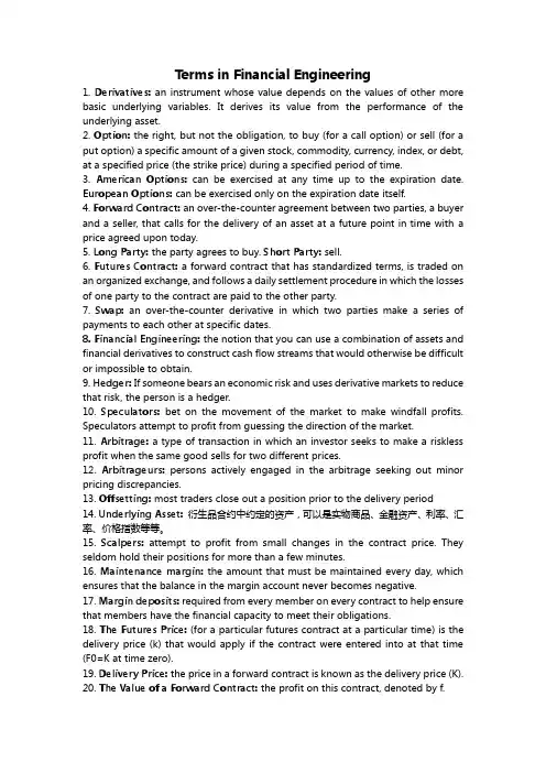
Terms in Financial Engineering1. Derivatives: an instrument whose value depends on the values of other more basic underlying variables. It derives its value from the performance of the underlying asset.2. Option: the right, but not the obligation, to buy (for a call option) or sell (for a put option) a specific amount of a given stock, commodity, currency, index, or debt, at a specified price (the strike price) during a specified period of time.3. American Options: can be exercised at any time up to the expiration date. European Options: can be exercised only on the expiration date itself.4. Forward Contract: an over-the-counter agreement between two parties, a buyer and a seller, that calls for the delivery of an asset at a future point in time with a price agreed upon today.5. Long Party: the party agrees to buy. Short Party: sell.6. Futures Contract: a forward contract that has standardized terms, is traded on an organized exchange, and follows a daily settlement procedure in which the losses of one party to the contract are paid to the other party.7. Swap: an over-the-counter derivative in which two parties make a series of payments to each other at specific dates.8. Financial Engineering: the notion that you can use a combination of assets and financial derivatives to construct cash flow streams that would otherwise be difficult or impossible to obtain.9. Hedger: If someone bears an economic risk and uses derivative markets to reduce that risk, the person is a hedger.10. Speculators: bet on the movement of the market to make windfall profits. Speculators attempt to profit from guessing the direction of the market.11. Arbitrage: a type of transaction in which an investor seeks to make a riskless profit when the same good sells for two different prices.12. Arbitrageurs: persons actively engaged in the arbitrage seeking out minor pricing discrepancies.13. Offsetting: most traders close out a position prior to the delivery period14. Underlying Asset: 衍生品合约中约定的资产,可以是实物商品、金融资产、利率、汇率、价格指数等等。
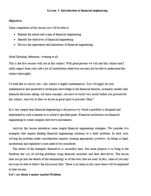
Lesson- 1: Introduction to financial engineeringObjectivesUpon completion of this lesson you will be able toExplain the nature and scope of financial engineeringIdentify the objectives of financial engineeringDiscuss the importance and limitations of financial engineeringGood Morning/ afternoon / evening to all.This is the first session with you in this subject. With good gesture we will start this subject and I really expect from your side a lot of contribution otherwise you may not be able to understand this subject thoroughly.I would like to convey you – this subject is highly mathematical. You will apply all your mathematical and quantitative techniques knowledge in the financial theories, economic models and financial decisions taking. All these concepts, you have to recall very nicely before you proceed for this subject. Anyway its fine we all are in good spirit to proceed. Okay?In a very simple term financial engineering is the process by which a portfolio is designed and maintained in such a manner as to achieve specified goals. Financial institutions use financial engineering to create complex derivative instruments.Anyway this lesson introduces some simple financial engineering strategies. We consider two examples that require finding financial engineering solutions to a daily problem. In each case, solving the problem under consideration requires creating appropriate synthetics. In doing so legal, institutional and regulatory issues need to be considered.The nature of the examples themselves is secondary here. Our main purpose is to bring to the forefront the way of solving problems using financial securities and their derivatives. The lesson does not go into the details of the terminology or of the tools that are used. In fact, some of you may not even be able to follow the discussion fully. There is no harm in this since these will be explained in later lessons.Let’s say about a money market ProblemConsider a Japanese bank in search of a 3-month money market loan. The bank would like to borrow U.S. dollars (USD) in Euromarkets and then on-lend them to its customers. This interbank loan will lead to cash flows as shown in Figure I-I. From the borrower's angle USD 100 is received at time to and then it is paid back with interest 3 months later at time t0 + δ. The interest rate is denoted by the symbol L to¼ and is determined at time t0. The tenor of the loan is 3 months. Thereforeδ = 14and the interest paid becomes L to ¼. The possibility of default is assumed away.Otherwise at time t0 + δ there would be a conditional cash flow depending on whether or not there is default.The money market loan displayed here is a fairly liquid instrument. In fact, banks purchase such "funds" in the wholesale interbank markets and then on-lend them to their customers at a slightly higher rate of interest.Now you see the ProblemSuppose the above mentioned Japanese bank finds out that this loan is not available due to the lack of appropriate credit lines. The counterparties are unwilling to extend the USD funds. The question then is: Are there other ways in which such dollar funding can be secured?The answer is yes. In fact, the bank can use foreign currency markets judiciously to construct exactly the same cash flow diagram as in Figure 1-1 and thus create a synthetic money market loan. This may seem an innocuous statement, but note that using currency markets and their derivatives will involve a completely different set of financial contracts, players, and institutional setup than the money markets. Yet, the result will be cash flows identical to those in Figure 1-1.We can come to the solution as:To see how a synthetic loan can be created, consider the following series of operations:1. The Japanese bank first borrows local funds in yen in the Japanese money markets. This is shown in the Figure. The bank receives yen at time t0 and will pay yen interest rate L y to.2. Next, the bank sells these yen in the spot market at the current exchange rate e to to secure USD 100. This spot operation is shown in the coming Figure.3. Finally, the bank must eliminate the currency mismatch introduced by these operations: In order to do this, the Japanese bank buys 100(1 + L toδ)f to yen at the known forward exchange rate fto' in the forward currency markets. This is the cash flow shown in the third Figure that follows. Here, there is no exchange of funds at time to. Instead, forward dollars will be exchanged for forward yen at t0 + δ.Now comes the critical point. In Figure two, add vertically all the cash flows generated by these operations. The yen cash flows will cancel out at time to because theyare of equal size and different sign. The time t0+ δyen cash flows will also cancel out because that is how the size of the forward contract is selected. The bank purchases just enough forward yen to pay back the local yen loan and the associated interest. The cash flows that are left are shown in fourth Figure and these are exactly the same cash flows as in Figure one. Thus, the three operations have created a synthetic USD loan.Here I would like to share with you some important ImplicationsThere are some subtle but important differences between the actual loan and the synthetic. First, note that from the point of view of euromarket banks, lending to Japanese banks involves a principal of USD 100, and this creates a credit risk. In case of default, the 100 dollars lent may not be repaid. Against this, some capital has to be put aside.Depending on the rate of money markets and depending on counterparty credit risks, money center banks may adjust their credit, lines toward such customers. .In contrast, in the case of the synthetic dollar loan, the international bank's exposure to the Japanese bank is in the forward currency market only. Here, there is no principal involved. If the Japanese bank defaults, the burden of default will be on the domestic banking system in Japan. There is a risk due to the forward currency operation, but it is a coul1terparty risk and is limited. Thus, the Japanese bank may end up getting the desired funds somewhat easier if a synthetic is used. .There is a second interesting point to the issue of credit risk mentioned earlier. The original money market loan was a Euromarket instrument. Banking operations in Euromarkets are considered offshore operations, taking place essentially outside the jurisdiction of national banking authorities. The local yen loan, on the other hand, is obtained in the onshore market. It would be subject to supervision by Japanese authorities. In ease of default, there may be some help from the Japanese Central Bank, unlike a Eurodollar loan where a default may have more severe implications on the lending bank.The third point has to do with pricing. If the actual and synthetic loans have identical cash flows, their values should also be the same excluding credit risk issues. Since, if there is a value discrepancy the markets will simultaneously sell the expensive one, and buy the cheaper one, realizing a windfall gain. This means that synthetics can also be used in pricing the original instrument. 2Fourth, note that the money market loan and the synthetic can in fact be each other's-hedge. Finally, in spite of the identical nature of the involved cash flows, the two ways of securing dollar funding happen in completely different markets and involve very different financial contracts. This means that legal and regulatory differences may be significant.Again let’s relate it to an Example of Taxation.Now consider a totally different problem. We create synthetic instruments to restructure taxable gains. The legal environment surrounding taxation being a complex and ever-changing phenomenon, this example should be read only from a financial engineering perspective and not as a tax strategy. Yet the example illustrates the close connection between what a financial engineer does and the legal and regulatory issues that surround this activity.The Problem Is:In taxation of financial gains and losses, there is a concept known as a wash-sale. Suppose that during the year 2002; an investor realizes some financial gains. Normally, these gains are taxable that year. But a variety of financial strategies can possibly be used to postpone taxation to the year after: To prevent such strategies, national tax authorities have a set of rules known as washsale, and stra4dle rules. It is important that professionals working for national tax authorities in various countries understand these strategies well and have a good knowledge of financial engineering. Otherwise some players may rearrange their portfolios, and this may lead to significant losses in tax revenues. From our perspective, we are concerned with the methodology of constructing synthetic instruments. This example will illustrate another such construction.Suppose that in September 2002, an investor bought an asset at a price So = $100. In December 2002, this asset is sold at S1 = $150. Thus, the investor has realized a capital gain of $50. These cash flows are shown in Figure 1-3. The first cash flow is negative and is placed below the time axis because it is a payment by the investor. The subsequent sale of the asset, on the other hand, is a receipt, and hence is represented by a positive cash flow placed above the time axis. The investor may have to pay significant taxes on these capital gains. A relevant question is then: Is it possible to use a strategy that postpones the investment gain to the next tax year?One may propose the following solution, however, is not permitted under the wash-sale rules. This investor is probably holding assets other than the S t mentioned earlier.After all, the right way to invest is to have diversifiable portfolios. It is also reasonable to assume that if there were appreciating assets such as S t, there were also assets that lost value during the same period. Denote the price of such an asset by Z t. Let the purchase price be Z0. If there were no wash-sale rules, the following strategy could be put together to postpone year 2002 taxes.Sell the Z-asset on December 2002, at a price Z1, Z l< Z0, and. the next day, buy the same Z t at a similar price. The sale will result in a loss equal toZ1 – Z0 < 0(2)The subsequent purchase puts this asset back into the portfolio so that the diversified portfolio can be maintained. This way, the losses in Z t are recognized and will cancel out some or all of the capital gains earned from S t. There may be several problems with this strategy, but one is fatal. Tax authorities would call this a wash-sale (i.e. a sale, that is being’. intentionally used to "wash" the 2002 capital gains) and would disallow the deductions.Another StrategyYet investors can find a way to sell the Z-asset without having to sell it in the usual way. This can be done by first creating a synthetic Z-asset and then realizing the implicit capital losses using this synthetic, instead of the Z-asset held in the portfolio. .Suppose the investor originally purchased the Z-asset at a price Z0= $100 and that' asset is currently trading at Z l = $50, with a paper loss of $50. The investor would like to recognize the loss without directly selling this asset. At the same time the investor would like to retain the original position in the Z-asset in order to maintain a well-balanced portfolio. How can the loss be realized while maintaining the Z-position and without selling the Z t ?The idea is to construct a proper synthetic. Consider the following sequence of operations:• Buy another Z-asset at price Z l = $50 on November 26, 2002. .• Sell an at-the-money call on Z with expiration date December 30, 2002.• Buy an at-the-money put on Z with the same expiration.The specifics of call and put options will be discussed in later chapters. For those readers' with no background in financial instruments we can add a few words. Briefly, options are instruments that give the purchaser a right. In the case of the call option, it is the right to purchase the underlying asset (here the Z-asset) at a pre-specified price (here $50). The put option is the opposite. It is the right to sell the asset at a pre-specified price (here $50). When one sells options, on the other hand, the seller has the obligation to deliver or accept delivery of the underlying at a pre-specified price.For our purposes, what is important is that short call and long put are two securities whose expiration payoff, when added will give the synthetic short position shown in Figure 1-4. By selling the call the investor has the obligation to deliver the Z-asset at a price of $50 if the call holder demands it. The put, on the other hand, gives the investor the right to sell the 2 -asset at $50 if he or she chooses to do so.The important point here is this: When the short call and the long put positions shown in Figure 1 -4 are added together the result will be equivalent to a short position on stock Z t. In fact, the investor has created a synthetic short position using options.Now consider what happens as time passes. If Z t appreciates by December 30, the call will be exercised. This is shown in Figure 1 -5a. The call position will lose money, since the investor has to deliver, at a loss, the original & Z stock that cost $100. If, on the other hand, the Z t decreases, then the put position will enable the investor to sell the original Z -stock at $50. This time the call will expire worthless.3 This situation is shown in Figure l-5b. Again, there will be a loss of $50. Thus, no matter what happens to the price Z t, either the investor will deliver the original Z-asset purchased at a price $100, or the put will be exercised and the investor will sell the original Z-asset at $50. Thus, one way or another, the investor is using the original asset purchased at $ 100 to close an option position at a loss. This means he or she will lose $50 while keeping the same & -position, since the second &, purchased at $50, will still be in the portfolio.The timing issue is important here. For example according to U.S. tax legislation, wash-sale rules will apply if the investor has acquired or sold a substantially identical property within a 3 I -day period. According to the strategy outlined here the second Z is purchased on November 26, while the options expire on December 30. Thus, there are more than 31 days between the two operations.ImplicationThere are at least three interesting points to our discussion. First, the strategy offered to the investor was risk-free and had zero cost aside from commissions and fees. Whatever happens to the new long position in the Z-asset, it will be canceled by the synthetic short position. This situation is shown in the lower half of Figure 1-4. As this graph shows, the proposed solution is risk less. The second point is that, once again, we have created a synthetic, and then used it in providing a solution to the tax problem. Finally, the example displays the crucial role legal and regulatory frameworks can play in devising financial strategies. Although this book does not deal with these issues, it is important to understand the crucial role they play at almost every level of financial engineering.Some Caveats for what is to follow for your proper understandingA newcomer to financial engineering usually follows instincts that are harmful for good understanding of the basic methodologies in the field. Hence, before we start, we need to layout some basic rules of the game that should be remembered throughout the book.1. This book is written from a market practitioner's point of view. Investors, pension funds, insurance companies, and governments are clients, and for us they are always on the other side of the deal. In other words, we look at financial engineering from a trader's, broker's and dealer's angle. The approach is from the manufacturer's perspective rather than the viewpoint of the user of the service. This premise is crucial in understanding some of the logic discussed in later chapters.2. We adopt the convention that there are two prices for every instrument unless stated otherwise. The agents involved in the deals often quote two-way prices. In economic theory, economic agents face the law of one price. The same good or asset cannot have two prices. If it did, we would then buy at the cheaper price and sell at the higher price.Yet in financial markets, there are two prices: one-price at which the financial market participant is willing to buy something from you, and another one at which the financial market participant is willing to sell the same thing to you. Clearly, the two cannot be the same. An automobile dealer will buy a used car at a low price in order to sell it at a higher price. That is how the dealer makes money. The same is true for a financial market practitioner. A swap dealer will be willing 10 buy swaps at a low price in order to sell them' at a higher price later. In the meantime, the instrument will be kept in the inventories, just like the used car sold to a car dealer. .3. A financial market participant is not an investor and never has "money." He or she has to secure funding for any purchase and has to place the cash generated by any sale. In. this book, almost no financial market operation begins with a pile of cash. The only "cash" is in the investor's hands, which in this book is on the other side of the transaction.It is for this reason that market practitioners prefer to work with instruments that have zero-value at the time of initiation. Such instruments would not require funding and are more practical to uses. They also are likely to have more liquidity.4. The role played by regulators professional organizations, and the legal profession is muchmore important for a market professional is much more important for an investor.Although it is far beyond the scope of this book, many financial engineering strategies have been devised for the sole purpose of dealing with them.Remembering these premises will greatly facilitate the understanding of financial engineering.。

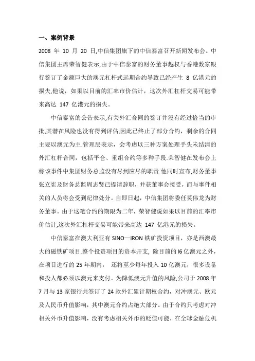
一、案例背景2008 年10 月20 日,中信集团旗下的中信泰富召开新闻发布会。
中信集团主席荣智健表示,由于中信泰富的财务董事越权与香港数家银行签订了金额巨大的澳元杠杆式远期合约导致已经产生8 亿港元的损失,他说,如果以目前的汇率市价估计,这次外汇杠杆交易可能带来高达147 亿港元的损失。
中信泰富的公告表示,有关外汇合同的签订并没有经过恰当的审批,其潜在风险也没有得到评估,因此已终止了部分合约,剩余的合同主要以澳元为主.管理层表示,会考虑以三种方案处理手头未结清的外汇杠杆合同,包括平仓、重组合约等多种手段.荣智健在发布会上称该事件中集团财务总监没有尽到应尽的职责.他同时宣布,财务董事张立宪及财务总监周志贤已提请辞职,并获董事会接受,而与事件相关的人员将会受到纪律处分。
自即日起,中信集团将委任莫伟龙为财务董事。
由于这笔合约的期限为二年,荣智健说如果以目前的汇率市价估计,这次外汇杠杆交易可能带来高达147 亿港元的损失。
中信泰富在澳大利亚有SINO—IRON铁矿投资项目,亦是西澳最大的磁铁矿项目.整个投资项目的资本开支, 除目前的l6亿澳元之外,在项目进行的25年期内,还将至少每年投入10亿澳元,很多设备和投人都必须以澳元来支付。
为降低澳元升值的风险,公司于2008年7月与13家银行共签订了24款外汇累计期权合约,对冲澳元、欧元及人民币升值影响,其中澳元合约占绝大部分。
由于合约只考虑对冲相关外币升值影响,没有考虑相关外币的贬值可能,在全球金融危机迫使澳大利亚减息并引发澳元下跌情况下,2008年10月20日中信泰富公告因澳元贬值跌破锁定汇价,澳元累计认购期权合约公允价值损失约147亿港元;11月14日中信泰富发布公告,称中信集团将提供总额为15亿美元(约ll6亿港元)的备用信贷,用于重组外汇衍生品合同的部分债务义务,中信泰富将发行等值的可换股债券,用来替换上述备用信贷.据香港《文汇报》报道, 随着澳元持续贬值,中信泰富因外汇累计期权已亏损186亿港元.截至2008年12月5日,中信泰富股价收于5.80港元,在一个多月内市值缩水超过2l0亿港元.另外,就中信泰富投资外汇造成重大亏损,并涉嫌信息披露延迟,香港证监会正对其展开调查。
END-OF-CHAPTER QUESTIONS AND PROBLEMSChapter 11. Business risk is the risk associated with a particular line of business, whereas financial risk is the risk associated with stock prices, exchange rates, interest rates and commodity prices. An example would be that a firm might be in the business of manufacturing furniture. Business risk would reflect the uncertainty of the furniture market, whereas financial risk would reflect the risk associated with the interest rates that would impact their borrowing costs. In addition a business might also be affected by exchange rates. Some of the financial risks can also be business risks. The business risk of a bank, for example, is highly affected by interest rate and exchange rate risk.2. Real assets consist of the tangible assets of the economy; however, for our purposes we also define them to include such intangible assets as management talent, ideas, brand names, etc. They are distinguished from financial assets, which are securities. These securities represent claims on business firms, which own the real assets, or on governments.3. An investor who is risk averse does not like risk and will not take on additional risk without the expectation of higher return. Such an individual will try to get the highest return for a given amount of risk or the lowest risk for a given amount of return. An individual who is risk neutral will simply seek the highest return without regard to risk.4. Financial markets distinguish the qualities of stocks and bonds by their prices. The markets set the price so that the return expected by investors is appropriate for the level of risk. In competitive and efficient markets, the expected return will vary directly with the level of risk. If one wishes to earn a higher return, it is necessary to assume more risk. This is the risk-return trade-off. Investors trade off risk against return.The risk-return trade-off will also hold in derivative markets. The risk-return trade-off is a fundamental result of the nature of competition in the marketplace. Attractive, low-risk investments will have their prices driven up and this will lower the expected returns. High-risk investments will have their prices driven down and this will result in higher expected returns.5. The expected return consists of the risk-free rate and a risk premium. The risk-free rate is the return one expects from investing money today and, thereby, foregoing the consumption that could be obtained. A risk premium is the additional return that one expects to receive by virtue of assuming risk.6. An efficient market is one in which prices reflect the true economic values of the assets trading therein. Inefficient markets, no one can earn returns that are more than commensurate with the level of risk. Efficient markets are characterized by low transaction costs and by the rapid rate at which new information is incorporated into prices.7. Arbitrage is a type of investment transaction that seeks to profit when identical goods are priced differently. Buying an item at one price and immediately selling it at another is a type of arbitrage. Because of the combined activities of arbitrageurs, identical goods, primarily financial assets, cannot sell for different prices for long. This is the law of one price. Arbitrage helps make our markets efficient by assuring that prices are in line with what they are supposed to be. In short, we cannot get something for nothing. A situation involving two identical goods or portfolios that are not priced equivalently would be exploited by arbitrageurs until their prices were equal. The "one price" that an asset must be is called the "theoretical fair value."11. Derivative markets provide a means of adjusting the risk of spot market investments to a more acceptable level and identifying the consensus market beliefs. They make trading easier and less costly and spot markets more efficient. These markets also provide a means of speculating.Chapter 33. European call: We know that its price cannot exceed S0 but must exceed Max(0, S0 - X(1+r)-T). With an infinite time to expiration, the present value of X is zero so the lower bound is S0 and, since the upper bound is S0, the call price must be S0. American call: We know that its price cannot exceed S0 but it must be at least as valuable as a European call. Thus its value must also be S0. Note that if exercised early it would be worth only S0 - X so it will never be exercised early.4. Ordinarily the option with the longer time to expiration would sell for more. If both options were deep out of-the-money, however, they could both sell for essentially nothing. The market would be expecting that both the shorter- and longer-lived options will expire out-of-the-money.5. If both options were deep out-of-the-money, they might have prices of zero. As in the previous question, the two options are expected to expire out-of-the-money.6. The call is underpriced, so buy the call, sell short the stock, and buy risk-free bonds with face value of X. The cash received from the stock is greater than the cost of the call and bonds. Thus, there is a positive cash flow up front. The payoffs from the portfolio at expiration are as follows:If S T < X,- S T (from the stock)X (from the bonds)the total, X - S T, is positive3-2If S T ≥ XS T - X (from the call)- S T (from the stock)X (from the bonds)the total is zero.The portfolio generates a positive cash flow up front and there is no cash outflow at expiration.7. Time value is a measure of the amount of uncertainty in an option. Uncertainty relates to whether the option will expire in- or out-of-the-money. When the option is deep in-the-money, there is little uncertainty about the fact that the option will expire in-the-money. The option will then begin to behave about like the stock. Then the option is deep-out-the-money, there is also little uncertainty since it is likely to finish out-of-the money. When the option is at-the-money there is considerable uncertainty about how it will finish.8. Assuming the stock pays no dividends, there is no reason to exercise a call early (this obviously presumes the call is American). The tendency to believe that exercising an option because the stock can go up no further ignores the fact that an option can generally be sold. Exercising an option throws away any chance that the stock can go up further. If the stock falls, the option holder would be hurt, but if the option holder exercised and became a stock holder, he would also be hurt by a falling stock price. There is simply no reason to give away the time value that arises because of the possibility that the stock can always go further upward. In simple, mathematical terms, exercising captures only the intrinsic value S0 - X. The call can always be sold for at least S0 - X (1 + r) -T.9. The paradox is resolved by recalling that if the option expires out-of-the-money, it does not matter how far out-of-the-money it is. The loss to the option holder is limited to the premium paid. For example, suppose the stock price is $24, the exercise price is $20, and the call price is $6. Higher volatility increases the chance of greater gains to the holder of the call. It also increases the chance of a larger stock price decrease. If, however, the stock price does end up below $20, the investor's loss is the same regardless of whether the stock price at expiration is $19 or $1. If the stock were purchased instead of the call, the loss would obviously be greater if the stock price went to $1 than if it went to $19. For this reason, holders of stocks dislike volatility, while holders of calls like volatility. A similar argument applies to puts.10. The minimum value of an American put is Max(0, X - S0). This is always higher than the lower bound of a European put, X (1 + r) -T - S0, except at expiration when the two are equal.11. When buying a call option, one hopes to exercise it at a later date. Thus, the exercise price will be paid out later. If interest rates are higher, additional interest can be earned on the money that will eventually be paid out as the exercise price. When buying a put option, one hopes to exercise it later, thus receiving the exercise price. If interest rates are higher, the put is less valuable because the holder is foregoing interest by having to wait to exercise the put. Higher interest rates make the present value of the exercise price be lower. In the case of the call, this is good because the call holder anticipates having to pay out the exercise price. For the put holder this is bad because the put holder anticipates receiving the exercise price.12. If the put price is higher than predicted by the model, the put is overpriced. Then the put should be sold. The funds should be used to construct a portfolio consisting of a long call and risk-free bonds with face value of X, and a short position in the stock. You can (and should) verify that this portfolio has a payoff at expiration that is the same as that of the put. Thus, if you sell the put for more than it costs to construct this portfolio, you can create a portfolio that offsets your put and have some money left over.13. An American call is exercised early only to capture a dividend. When a stock goes ex-dividend, the call will lose value as the stock drops. This will cause a loss in value to the holder of the call. The call holder knows this loss will be incurred as soon as the stock goes ex-dividend. If the call were exercised just before the stock goes ex-dividend, however, the call holder would capture the stock and the dividend, which might be enough to offset the otherwise loss in the value of the call. For a put, however, dividends are not necessary to make the argument that it might be optimal to exercise early. The holder of an American put faces a situation in which the gains are limited to the exercise price. Since the stock price can go down only to zero, early exercise of a put on a bankrupt firm would obviously be advisable. But the firm does not have to go bankrupt. If the stock price is low enough, the gains from waiting for it to go lower are not worth the wait. If dividends were added to the picture, however, they would discourage early exercise. The more dividends paid, the lower the stock price is driven and the more valuable it is to hold on to the put.Chapter 41. When we price an option according to its boundary conditions, we do not find an exact price for the option. We provide only limits on the maximum and minimum price of an option or group of options. In the case of options differing by exercise prices or in the case of put-call parity, we can price only the relationship or difference between the option prices. We cannot price each option individually without an option pricing odel; however, an option pricing model must provide prices that conform to the boundary conditions. Because boundary condition rules require fewer assumptions, we can say that they are more generally applicable and are more likely to hold in practice. They are incomplete, however, in the sense that they do not tell us exactly what the option price should be, which is what an option pricing model does tell us.2. A binomial option pricing model enables us to see the relationship between the stock price and the call price. The model shows, in a simple framework, how to construct a riskless portfolio by appropriately weighting the stock against the option. By noting that the riskless portfolio should return the risk-free rate, we can see what the call price must be. We can also understand the forces that bring the call option price in line if it is not priced according to the model. In addition, the model illustrates the importance of revising the hedge ratio. Finally, the model is probably the best way to handle the problem of pricing an American option.3. For a call, a hedge portfolio will consist of n shares of stock and one short call. The shares of stock, n, will be a long position that will reflect the next two possible values of the call and stock. The call is short because the call and stock move opposite each other, so a short position in the call is needed to offset a long position in the stock. If the option is a put, a long position in n shares will be hedged by a long position in one put. The number of shares, n, is also a reflection of the next two possible option and stock values. The put is long because it already moves opposite to the stock.4. This means that the option is trading in the market for a price that is lower than its theoretical fair value. Consequently, the option is underpriced. An underpriced option should be bought. To hedge the position, one should sell n shares of stock, where n is the hedge ratio as defined in the chapter.5. At each point in the binomial tree, the option price is computed based on the next two possible prices, weighted by the appropriate probability values and discounted back one period. If the option can be exercised early, we determine its intrinsic value, i.e., the value it would have if it were exercised at that point. If the intrinsic value is greater, it replaces the computed value. This is done at all nodes. Note that it is quite possible that the option will be exercised at many different nodes.6. A path independent problem is one in which the only values that matter in determining the current price are the values at expiration. A particular expiration value is the same regardless of the sequence of up and down moves the stock took to get to that point. A path dependent model is one in which the sequence of up and down moves does matter. For example, suppose the stock goes down, up and then up. Contrast that with up, up and down. If the option is a European put, it does not matter which sequence the stock followed. Where it is at expiration is the only thing that matters. If the option is, however, an American put, the down, up, up sequence could lead to early exercise when it makes that first move down, whereas the up, up, down sequence is unlikely to lead to early exercise.Chapter 51. In a discrete time model, the stock price can make a jump to only one of two possible values. The length of time over which the move can be made is finite. In a continuous time model, the stock price can jump to an infinite number of possibilities. The length of time over which the move can be made is infinitesimal (very, very small). The difference between the two models is perhaps best described as in the text as the difference between still photos and a movie.2. The familiar normal or bell-shaped distribution is a symmetric probability distribution that depends only on the mean and variance. A lognormal distribution is skewed, having more extreme right values. A lognormal distribution, however, is normal in the logarithm. Thus, if x is lognormally distributed, its logarithm, lnx, is normally distributed. With respect to stock prices, the logarithm is of the rate of return. That is, let (S1 –S0)/S0 be defined as the return over period 0 to period 1. Then if it is lognormally distributed, ln(S1/S0) is normally distributed. Note what appears to be slight inconsistency: (S1 – S0)/S0 is a percentage return whereas S1/S0 is 1.0 plus the percentage return. That does not matter as we can always shift a normal distribution by adding a constant such as 1.0 and it does not affect the fact that it is normally distributed. It just slides it over.3. The Black-Scholes model assumes no dividends, but actually this was just for convenience to allow us to start at the simplest level. If the dividends are appropriately modeled, the Black-Scholes model handles stocks with dividends with only the minor adjustment that we must remove the present value of the dividends from the stock price before using it in the model. We can do this by subtracting the present value of the stream of discrete dividends over the life of the model or by discounting the stock price by the dividend yield rate over the life of the model.4. The variables in the binomial model are S0 (the stock price), X (the exercise price), r (the discrete risk-free rate), u (one plus the return on the stock if it goes up), d (one plus the return on the stock if it goes down) and n, the number of time periods. The variables in the Black-Scholes model are S0 (the stock price), X (the exercise price), r c (the continuously compounded risk-free rate), ó (the standard deviation of the continuously compounded return on the stock) and T (the time to expiration). The variables S0 and X are the same in both models. In the binomial model, r is the discrete interest rate per period. In the Black-Scholes model, the interest rate must be expressed in continuously compounded form. The annual discrete interest rate (r) is related to the annual continuously compounded rate (r c) by the formula, r c = ln(1 + r). Then the binomial rate per period is found as (1 + r)T/n - 1. The up and down factors in the binomial model are directly related to ó in the Black-Scholes model by the formula u = T/n ó e – 1 and d = (1/(1+u)) – 1. The time to expiration (T) in the Black-Scholes model is related to the length of each binomial period by the relationship T/n where n is the number of periods. Thus, all of the Black-Scholes variables are either equal to or directly convertible to binomial variables.Chapter6Chapter7Chapter 8Chapter9Chapter 10。
END-OF-CHAPTER QUESTIONS AND PROBLEMSChapter 11. Business risk is the risk associated with a particular line of business, whereas financial risk is the risk associated with stock prices, exchange rates, interest rates and commodity prices. An example would be that a firm might be in the business of manufacturing furniture. Business risk would reflect the uncertainty of the furniture market, whereas financial risk would reflect the risk associated with the interest rates that would impact their borrowing costs. In addition a business might also be affected by exchange rates. Some of the financial risks can also be business risks. The business risk of a bank, for example, is highly affected by interest rate and exchange rate risk.2. Real assets consist of the tangible assets of the economy; however, for our purposes we also define them to include such intangible assets as management talent, ideas, brand names, etc. They are distinguished from financial assets, which are securities. These securities represent claims on business firms, which own the real assets, or on governments.3. An investor who is risk averse does not like risk and will not take on additional risk without the expectation of higher return. Such an individual will try to get the highest return for a given amount of risk or the lowest risk for a given amount of return. An individual who is risk neutral will simply seek the highest return without regard to risk.4. Financial markets distinguish the qualities of stocks and bonds by their prices. The markets set the price so that the return expected by investors is appropriate for the level of risk. In competitive and efficient markets, the expected return will vary directly with the level of risk. If one wishes to earn a higher return, it is necessary to assume more risk. This is the risk-return trade-off. Investors trade off risk against return.The risk-return trade-off will also hold in derivative markets. The risk-return trade-off is a fundamental result of the nature of competition in the marketplace. Attractive, low-risk investments will have their prices driven up and this will lower the expected returns. High-risk investments will have their prices driven down and this will result in higher expected returns.5. The expected return consists of the risk-free rate and a risk premium. The risk-free rate is the return one expects from investing money today and, thereby, foregoing the consumption that could be obtained. A risk premium is the additional return that one expects to receive by virtue of assuming risk.6. An efficient market is one in which prices reflect the true economic values of the assets trading therein. Inefficient markets, no one can earn returns that are more than commensurate with the level of risk. Efficient markets are characterized by low transaction costs and by the rapid rate at which new information is incorporated into prices.7. Arbitrage is a type of investment transaction that seeks to profit when identical goods are priced differently. Buying an item at one price and immediately selling it at another is a type of arbitrage. Because of the combined activities of arbitrageurs, identical goods, primarily financial assets, cannot sell for different prices for long. This is the law of one price. Arbitrage helps make our markets efficient by assuring that prices are in line with what they are supposed to be. In short, we cannot get something for nothing. A situation involving two identical goods or portfolios that are not priced equivalently would be exploited by arbitrageurs until their prices were equal. The "one price" that an asset must be is called the "theoretical fair value."11. Derivative markets provide a means of adjusting the risk of spot market investments to a more acceptable level and identifying the consensus market beliefs. They make trading easier and less costly and spot markets more efficient. These markets also provide a means of speculating.Chapter 33. European call: We know that its price cannot exceed S0 but must exceed Max(0, S0 - X(1+r)-T). With an infinite time to expiration, the present value of X is zero so the lower bound is S0 and, since the upper bound is S0, the call price must be S0. American call: We know that its price cannot exceed S0 but it must be at least as valuable as a European call. Thus its value must also be S0. Note that if exercised early it would be worth only S0 - X so it will never be exercised early.4. Ordinarily the option with the longer time to expiration would sell for more. If both options were deep out of-the-money, however, they could both sell for essentially nothing. The market would be expecting that both the shorter- and longer-lived options will expire out-of-the-money.5. If both options were deep out-of-the-money, they might have prices of zero. As in the previous question, the two options are expected to expire out-of-the-money.6. The call is underpriced, so buy the call, sell short the stock, and buy risk-free bonds with face value of X. The cash received from the stock is greater than the cost of the call and bonds. Thus, there is a positive cash flow up front. The payoffs from the portfolio at expiration are as follows:If S T < X,- S T (from the stock)X (from the bonds)the total, X - S T, is positive3-2If S T ≥ XS T - X (from the call)- S T (from the stock)X (from the bonds)the total is zero.The portfolio generates a positive cash flow up front and there is no cash outflow at expiration.7. Time value is a measure of the amount of uncertainty in an option. Uncertainty relates to whether the option will expire in- or out-of-the-money. When the option is deep in-the-money, there is little uncertainty about the fact that the option will expire in-the-money. The option will then begin to behave about like the stock. Then the option is deep-out-the-money, there is also little uncertainty since it is likely to finish out-of-the money. When the option is at-the-money there is considerable uncertainty about how it will finish.8. Assuming the stock pays no dividends, there is no reason to exercise a call early (this obviously presumes the call is American). The tendency to believe that exercising an option because the stock can go up no further ignores the fact that an option can generally be sold. Exercising an option throws away any chance that the stock can go up further. If the stock falls, the option holder would be hurt, but if the option holder exercised and became a stock holder, he would also be hurt by a falling stock price. There is simply no reason to give away the time value that arises because of the possibility that the stock can always go further upward. In simple, mathematical terms, exercising captures only the intrinsic value S0 - X. The call can always be sold for at least S0 - X (1 + r) -T.9. The paradox is resolved by recalling that if the option expires out-of-the-money, it does not matter how far out-of-the-money it is. The loss to the option holder is limited to the premium paid. For example, suppose the stock price is $24, the exercise price is $20, and the call price is $6. Higher volatility increases the chance of greater gains to the holder of the call. It also increases the chance of a larger stock price decrease. If, however, the stock price does end up below $20, the investor's loss is the same regardless of whether the stock price at expiration is $19 or $1. If the stock were purchased instead of the call, the loss would obviously be greater if the stock price went to $1 than if it went to $19. For this reason, holders of stocks dislike volatility, while holders of calls like volatility. A similar argument applies to puts.10. The minimum value of an American put is Max(0, X - S0). This is always higher than the lower bound of a European put, X (1 + r) -T - S0, except at expiration when the two are equal.11. When buying a call option, one hopes to exercise it at a later date. Thus, the exercise price will be paid out later. If interest rates are higher, additional interest can be earned on the money that will eventually be paid out as the exercise price. When buying a put option, one hopes to exercise it later, thus receiving the exercise price. If interest rates are higher, the put is less valuable because the holder is foregoing interest by having to wait to exercise the put. Higher interest rates make the present value of the exercise price be lower. In the case of the call, this is good because the call holder anticipates having to pay out the exercise price. For the put holder this is bad because the put holder anticipates receiving the exercise price.12. If the put price is higher than predicted by the model, the put is overpriced. Then the put should be sold. The funds should be used to construct a portfolio consisting of a long call and risk-free bonds with face value of X, and a short position in the stock. You can (and should) verify that this portfolio has a payoff at expiration that is the same as that of the put. Thus, if you sell the put for more than it costs to construct this portfolio, you can create a portfolio that offsets your put and have some money left over.13. An American call is exercised early only to capture a dividend. When a stock goes ex-dividend, the call will lose value as the stock drops. This will cause a loss in value to the holder of the call. The call holder knows this loss will be incurred as soon as the stock goes ex-dividend. If the call were exercised just before the stock goes ex-dividend, however, the call holder would capture the stock and the dividend, which might be enough to offset the otherwise loss in the value of the call. For a put, however, dividends are not necessary to make the argument that it might be optimal to exercise early. The holder of an American put faces a situation in which the gains are limited to the exercise price. Since the stock price can go down only to zero, early exercise of a put on a bankrupt firm would obviously be advisable. But the firm does not have to go bankrupt. If the stock price is low enough, the gains from waiting for it to go lower are not worth the wait. If dividends were added to the picture, however, they would discourage early exercise. The more dividends paid, the lower the stock price is driven and the more valuable it is to hold on to the put.Chapter 41. When we price an option according to its boundary conditions, we do not find an exact price for the option. We provide only limits on the maximum and minimum price of an option or group of options. In the case of options differing by exercise prices or in the case of put-call parity, we can price only the relationship or difference between the option prices. We cannot price each option individually without an option pricing odel; however, an option pricing model must provide prices that conform to the boundary conditions. Because boundary condition rules require fewer assumptions, we can say that they are more generally applicable and are more likely to hold in practice. They are incomplete, however, in the sense that they do not tell us exactly what the option price should be, which is what an option pricing model does tell us.2. A binomial option pricing model enables us to see the relationship between the stock price and the call price. The model shows, in a simple framework, how to construct a riskless portfolio by appropriately weighting the stock against the option. By noting that the riskless portfolio should return the risk-free rate, we can see what the call price must be. We can also understand the forces that bring the call option price in line if it is not priced according to the model. In addition, the model illustrates the importance of revising the hedge ratio. Finally, the model is probably the best way to handle the problem of pricing an American option.3. For a call, a hedge portfolio will consist of n shares of stock and one short call. The shares of stock, n, will be a long position that will reflect the next two possible values of the call and stock. The call is short because the call and stock move opposite each other, so a short position in the call is needed to offset a long position in the stock. If the option is a put, a long position in n shares will be hedged by a long position in one put. The number of shares, n, is also a reflection of the next two possible option and stock values. The put is long because it already moves opposite to the stock.4. This means that the option is trading in the market for a price that is lower than its theoretical fair value. Consequently, the option is underpriced. An underpriced option should be bought. To hedge the position, one should sell n shares of stock, where n is the hedge ratio as defined in the chapter.5. At each point in the binomial tree, the option price is computed based on the next two possible prices, weighted by the appropriate probability values and discounted back one period. If the option can be exercised early, we determine its intrinsic value, i.e., the value it would have if it were exercised at that point. If the intrinsic value is greater, it replaces the computed value. This is done at all nodes. Note that it is quite possible that the option will be exercised at many different nodes.6. A path independent problem is one in which the only values that matter in determining the current price are the values at expiration. A particular expiration value is the same regardless of the sequence of up and down moves the stock took to get to that point. A path dependent model is one in which the sequence of up and down moves does matter. For example, suppose the stock goes down, up and then up. Contrast that with up, up and down. If the option is a European put, it does not matter which sequence the stock followed. Where it is at expiration is the only thing that matters. If the option is, however, an American put, the down, up, up sequence could lead to early exercise when it makes that first move down, whereas the up, up, down sequence is unlikely to lead to early exercise.Chapter 51. In a discrete time model, the stock price can make a jump to only one of two possible values. The length of time over which the move can be made is finite. In a continuous time model, the stock price can jump to an infinite number of possibilities. The length of time over which the move can be made is infinitesimal (very, very small). The difference between the two models is perhaps best described as in the text as the difference between still photos and a movie.2. The familiar normal or bell-shaped distribution is a symmetric probability distribution that depends only on the mean and variance. A lognormal distribution is skewed, having more extreme right values. A lognormal distribution, however, is normal in the logarithm. Thus, if x is lognormally distributed, its logarithm, lnx, is normally distributed. With respect to stock prices, the logarithm is of the rate of return. That is, let (S1 –S0)/S0 be defined as the return over period 0 to period 1. Then if it is lognormally distributed, ln(S1/S0) is normally distributed. Note what appears to be slight inconsistency: (S1 – S0)/S0 is a percentage return whereas S1/S0 is 1.0 plus the percentage return. That does not matter as we can always shift a normal distribution by adding a constant such as 1.0 and it does not affect the fact that it is normally distributed. It just slides it over.3. The Black-Scholes model assumes no dividends, but actually this was just for convenience to allow us to start at the simplest level. If the dividends are appropriately modeled, the Black-Scholes model handles stocks with dividends with only the minor adjustment that we must remove the present value of the dividends from the stock price before using it in the model. We can do this by subtracting the present value of the stream of discrete dividends over the life of the model or by discounting the stock price by the dividend yield rate over the life of the model.4. The variables in the binomial model are S0 (the stock price), X (the exercise price), r (the discrete risk-free rate), u (one plus the return on the stock if it goes up), d (one plus the return on the stock if it goes down) and n, the number of time periods. The variables in the Black-Scholes model are S0 (the stock price), X (the exercise price), r c (the continuously compounded risk-free rate), ó (the standard deviation of the continuously compounded return on the stock) and T (the time to expiration). The variables S0 and X are the same in both models. In the binomial model, r is the discrete interest rate per period. In the Black-Scholes model, the interest rate must be expressed in continuously compounded form. The annual discrete interest rate (r) is related to the annual continuously compounded rate (r c) by the formula, r c = ln(1 + r). Then the binomial rate per period is found as (1 + r)T/n - 1. The up and down factors in the binomial model are directly related to ó in the Black-Scholes model by the formula u = T/n ó e – 1 and d = (1/(1+u)) – 1. The time to expiration (T) in the Black-Scholes model is related to the length of each binomial period by the relationship T/n where n is the number of periods. Thus, all of the Black-Scholes variables are either equal to or directly convertible to binomial variables.Chapter6Chapter7Chapter 8Chapter9Chapter 10。

金融工程原理英文版第二版课程设计IntroductionFinancial engineering is a multidisciplinary field that combines principles of finance, economics, mathematics, statistics, and computer science to design and develop financial products, strategies, and systems. The field has grown rapidly in recent years due to the increasing complexity of financial markets and the need for sophisticated tools and techniques to manage financial risk and create value. In this course, we will introduce the fundamental principles of financial engineering and explore how they can be applied to real-world problems and scenarios.Course ObjectivesThe course is designed to provide students with a comprehensive understanding of the principles and practices of financial engineering. Specifically, the course ms to:•Introduce students to the basic concepts and terminologies of financial engineering•Provide students with a strong foundation in mathematical and statistical techniques used in financial engineering•Explore the various financial products and instruments used in financial markets, including equities, bonds, options, andfutures•Discuss the techniques and strategies used in financial risk management, including value-at-risk (VaR), stress testing, andhedging•Examine the role of financial engineering in asset pricing, portfolio optimization, and investment management.Course OutlineThe course will cover the following topics:Week 1: Introduction to Financial Engineering•Definition of financial engineering•The history and evolution of financial engineering•The role of financial engineering in modern financeWeek 2: Mathematical Foundations•Basic statistics and probability theory•The Black-Scholes-Merton model and its applications•Stochastic calculus and Ito’s lemmaWeek 3: Financial Markets and Instruments•Equities and derivatives•Fixed income securities and instruments•Options and futuresWeek 4: Financial Risk Management•Value-at-Risk (VaR) and its applications•Portfolio optimization and diversification•Hedging strategiesWeek 5: Asset Pricing and Investment Management•Capital asset pricing model (CAPM) and efficient frontier•Arbitrage pricing theory (APT) and security valuation•Portfolio management techniquesWeek 6: Course Review and Evaluation•Review of course materials and concepts•Evaluation of student performance and achievement•Discussion of future directions and opportunities in financial engineeringCourse RequirementsThe course is open to students from all majors, but it is recommended that students have a strong background in mathematics, statistics, and finance. Students will be expected to attend lectures, participate in class discussions and group activities, and complete assignments and exams.Textbook and MaterialsThe required textbook for the course is Financial Engineering: Principles and Strategies by Robert Korajczyk. In addition, students will need access to a computer with statistical software (such as R or MATLAB) and Excel.ConclusionFinancial engineering is a rapidly evolving field that offers exciting opportunities for students interested in pursuing careers in finance, economics, mathematics, and computer science. This course will provide students with a comprehensive understanding of the principles and practices of financial engineering, as well as the practical skills and knowledge needed to excel in this dynamic and challenging field.。
Waldo CountyWald County, the well-known real estate developer, worked long hours, and he expected his staff to do the same1></a>. So George was about to leave for a long summer’s weekend.Mr. County’ s success had been built on a remark able instinct for a good site. He would exclaim “location! location! location!”at some point in every planning meeting. Yet finance was not his strong suit. On this occasion he wanted George to go over the figures for a new $90 million outlet mall designed to intercept tourists heading downeast toward Maine. “I’ll be in my house in Bar Harbor if you need me.”George’s first task was to draw up a summary of the projected revenues and costs. The results are shown in Table 10.7. Note that the mall’ s revenues would come from two sources: The company would come from two sources: The company would charge retailers an annual rent for the space they occupied and in addition it would receive 5 percent of each store’s gross sales.Construction of the mail was likely to take three years. The construction costs could be depreciated straight-line over 15 years starting in year 3. As in the case of the company’s other developments, the mall would be built to the highest specifications and would not need to be rebuilt until year 17. The land was expected to retain its value, but could not be depreciated for tax purposes.Construction costs, revenues, operating and maintenance costs, and real estate taxes were all likely to rise in line with inflation, which was forecasted at 2 percent a year. The company’s tax rate was 35 percent and the cost of capital was 9 percent in nominal terms.George decided first to check that the project made financial sense. He then proposed to look at some of the things that might go wrong. His boss certainly had nose for a good retail project, but he was not infallible. The Salome project had been a disaster because store sales had turned to be 40 percent below forecast. What if that happened here? George wondered just how far sales could fall short of forecast before the project would be underwater.TABLE 10.7Projected revenues and costs in real terms for the Downeast Tourist Mall(figures in $millions)YEAR1345-17Investment:Land30Construction203010Operations:Rentals121212Share of retail sales24224Operating and maintenance costs 244101010Real estate taxes22444Inflation was another source of uncertainty. Some people were talking about a zero long-term inflation rate, but George also wondered what would happen if inflation jumped to, say, 10 percent.A third concern was possible construction cost overruns and delays due to required zoning changes and environmental approvals. George had seen cases of 25 percent construction cost overruns and delays up to 12 months between purchase of the land and the start of construction. He decided that he should examine the effect that this scenario would have on the project’s profitability.“Hey, this might be fun,” George exclaimed to Mr. Waldo’s secretary, Fifi, who was heading for Old Orchard Beach for the weekend. “I might even try Monte Carlo.”“Waldo went to Monte Carlo once,” Fifi replied. “Lost a bundle at the roulette table. I wouldn’t remind him. Just show him the bottom line.”“OK, no Monte Carlo,” George agreed. But he realized that building a spreadsheet and running scenarios was not enough. He had to figure out how to summarize and present his results to Mr. Country.。