modelmuse地下水模拟软件教程
- 格式:pdf
- 大小:1.36 MB
- 文档页数:59

地下水模拟软件GMS中文使用手册地下水模拟是一种基于数学模型的水文学研究方法,通过模拟不同地下水流动情况,可以更好地了解地下水资源分布和变化规律,为工程建设和保护提供科学依据。
而在地下水模拟中,GMS是一个常用的软件工具,它可以用来建立和分析多种类型的地下水流动模型。
本篇文章将详细介绍GMS软件的基本操作和常用功能,以及地下水模拟的一些注意事项。
一、GMS软件介绍GMS即Groundwater Modeling System,是一款专业的地下水模拟软件,拥有强大的建模分析能力。
GMS可以创建多种类型的地下水模型,包括层状模型、地下水盆地模型、地下水河道模型等。
同时,GMS还拥有强大的数据处理和可视化功能,可以方便地将地下水模型的结果呈现出来。
二、GMS基本操作1、软件安装和启动下载GMS软件后,按照提示进行安装即可。
启动软件后,可以选择新建、打开或最近使用的工程文件。
2、新建工程在GMS中,地下水模型被称为“工程”,因此需要新建一个工程来开始建模。
点击菜单栏的“文件”>“新建工程”,然后设置工程名称、模型类型等参数即可。
3、添加模型在新建工程后,需要添加一个地下水模型。
点击“地下水模型”>“新建”来创建模型,选择模型类型和分析区域范围,然后导入数据(如DEM图像、土壤信息等)。
4、设置材料属性在添加地下水模型后,需要为各个材料设置属性(如渗透系数、孔隙度等),以方便地进行模拟分析。
点击“属性”>“材料属性”来设置材料属性。
5、添加边界条件和压头在进行地下水模拟时,需要将分析范围分为不同的区域,并分别设置边界条件和压头。
点击“水头”>“边界条件”和“水头”>“压头”,在地图上分别添加边界条件和压头所在的点。
6、生成计算网格在设置好材料属性、边界条件和压头后,需要生成计算网格来进行模拟分析。
点击“计算网格”>“自动生成”来生成计算网格,并根据需要进行调整。
7、设置时间步长在进行地下水模拟时,需要设置时间步长和时间范围,以控制分析精度和时间范围。


SMS地表水模拟软件的使用说明SMS是英文Surface Water Modeling System(地表水模拟系统)首个字母的组合,是美国陆军工程兵水利工程实验室(United States Army Corps of Engineers Hydraulics Laboratory)和扬·伯明翰大学(Brigham Young University)等合作开发的商业软件,可用来模拟水体的流场和浓度场。
它由FESWMS-2DH、RMA2、RMA4、SED2D等软件包组成。
本章对将使用的RMA2和RMA4软件包及其强大的后处理功能作较详细地说明。
1 水动力模型的建立水动力模型建立的步骤如图1所示:图1 RMA2二维水动力模型的工作流程1.1 输入底图采用SMS进行地表水模拟时,首先要输入较详细的底图。
SMS8.1软件输入底图的途径主要有两种:一、打开tiff格式的图形文件,将地图中随机的三点的坐标输入定位,使底图与实际地形吻合;二、此外SMS8.1软件还支持AutoCAD转换成的R12的.dxf格式的电子地图,可以直接打开.dxf格式的地图。
1.2定义节点具体操作如下:1、点击图标增加节点,利用图标选择节点,以便对节点进行修改;2、选中两节点,在SMS8.1版本中在窗口下方偏右出现distance项为两节点距离,如图2所示。
已知两点距离,可在Node/Interpolation Option项中调整插入的节点数,根据实际情况插入节点。
3、节点坐标包括x、y、z值可在坐标框中输入,确定节点的确切位置及高程,如图3所示。
图2两节点间距离显示图图3节点坐标显示图1.3 构建网格1.3.1 网格的构建应满足以下条件:1、据水力特征流速大小和过水能力的大小使网格疏密有致;2、构建模型者所估计的流线平行;3、三角形与四边形注意过渡。
边界、流场复杂区域用三角形,流速均匀、航道、湖区等地使用四边形。
1.3.2 构建方法:1、手动添加网格单元: 选中三个节点,点击,形成形如图标的六节点三角形网格;选中四个节点,点形成八节点的四边形网格;点分割四边形网格或将两相邻的三角形网格合成为四边形网格;点将内含两个三角形网格的四边形网格调转方向,使得网格满足适应流线,避免出现网格质量的原则。
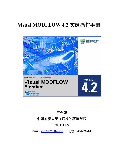
Visual MODFLOW 4.2实例操作手册王全荣中国地质大学(武汉)环境学院2011-11-5Emil: wqr88@ QQ:283278961引言MODFLOW是英文名称Modular Three-dimensional FiniteDifference Groundwater flow model (三维有限差分地下水流模型)的简称。
由美国地质调查局(Unite State Geological Survey)于80 年代开发出的一套专门用于孔隙介质中地下水流动相关问题数值模拟的软件。
自问世以来,MODFLOW 已经在全世界范围内,在科研、生产、环境保护、城乡发展规划、水资源利用等许多行业和部门得到了广泛的应用,是供水文地质工作者使用的一套功能强大的实用计算机软件。
同时,MODFLOW软件的源代码可以在美国内政部网站上免费下载,供水文地质工作者参考和修改,以提高数值模拟的仿真性。
Visual MODLFOW软件中不仅包括MODLFOW模块,还有SEAWAT、MT3D、MODPATH等模块。
为了让广大水文地质工作者能快速入门并精通该数值模拟软件,作者参考相关文献分别针对上述的模块自拟几个实例,并给出相应的操作步骤,供大家练习参考。
作者:王全荣2011年11月目录实例1 地下水流-污染物迁移规律数值模拟实例 (4)1、实例模型背景介绍及概念模型 (4)2、VM软件模拟该问题所需要的资料以及资料整理格式 (5)2.1数值模拟资料 (5)2.2资料整理格式 (5)3、VM软件模拟地下水流场:F LOW F IELD (6)3.1新建工程项目 (6)3.2模块I:模型输入 (8)3.3模块II:计算(Run) (23)3.4模块III:输出的可视化 (24)3.5模型校正 (26)4、VM软件模拟地下水流迹线:MODPATH.............................................................错误!未定义书签。
第一卷第二章用TINs(不规则三角网)做地表模型GMS中的TIN模块是用来做通用的地表模型。
TIN是不规则三角网,是由一系列三角形的x,y,z点形成的,被认为是随着每个三角形线性的变化。
TINs 可以被用来代表一个地质单元,地表可以用一个数学方程来定义。
TIN上的高程或者其他值可以用等值线的形式显示,TINs被用来构建实体模型和三维有限元网格。
2.1开始2.2需要的模块和界面●Sub-surface 特征●Geostatistics地质统计学2.3导入节点1.切换到TIN模块。
2.选择打开按钮。
3.在打开对话框中,定位到路径tutfiles\tins。
4.选择verts.gpr,然后点击打开。
在屏幕上就会出现一系列的点,这些点还没有被三角形连接起来。
2.4三角化为了建立一个三角网,我们必须三角化我们导入的节点。
三角化这些节点:1.选择BuildTINs|Triangulate命令。
节点应该和边界连接起来以便建立一个三角网。
三角化是通过Delaunay 方法自动的插值实现的。
2.5等值线现在三角网已经建好了,我们可以用TIN的高程来建立一个等值线图。
1.选择显示按钮。
2.选中Contour和TIN边界选项,取消三角网边界和节点选项。
3.选择OK按钮。
等值线已经生成了,假设TINs根据地表每个三角网线性的变化。
2.6光亮另外的显示TIN的方法是用光源。
1.选择显示按钮。
2.关闭等值线和TIN边界选项,然后选中三角形面的选项。
3.选择ok按钮。
4.选择三维显示按钮。
5.选择“Display”菜单下面得到“光照”命令。
6.改变光照的角度为0.7,然后点击ok。
7.选择旋转工具,然后在图形窗口中拖动鼠标,旋转视角。
2.7编辑TIN因为TIN是被用来建立实体和网格的,一旦它建立以后通常要修改一下,在大多数情况下,TINS都是由离散点生成的。
1.选择显示选项“Display option”。
2.选中Vertices和Contour选项。
地下水数值模拟任务步骤及常用软件地下水数值模拟是指通过建立数学模型和运用计算机方法,利用计算机模拟地下水的水文过程,预测地下水的动态变化,并定量分析地下水资源的开发利用。
地下水数值模拟在地下水资源管理、环境保护、地下水污染防治等领域具有广泛的应用。
1.建立地下水数学模型:根据地下水的特征和要研究的问题,建立合适的数学方程和边界条件,描述地下水系统的基本运动规律。
2.选择合适的计算方法:根据模型的特征和要求,选择合适的数值计算方法,如有限差分法、有限元法、边界元法等。
3.模型参数的确定:对于地下水数学模型中的一些参数,如渗透率、初始压力等,需要通过现场实测或实验室测试获得,并进行合理的插值和外推处理。
4.数值模拟的实施和验证:利用计算机软件进行数值计算,模拟地下水系统的动态变化,并通过对模拟结果的与实测数据的比较,验证模型的可靠性和准确性。
5.模型的应用和优化:在模型建立和验证的基础上,利用模型进行不同方案的对比研究,优化地下水资源的管理和利用方式。
1.MODFLOW:是美国地质调查局开发的地下水流动模型,是目前最常用的三维地下水数值模拟软件之一、具有强大的建模和计算功能,可以模拟各种地下水问题。
2. FEFLOW:是德国DHIGmbH公司开发的强大的地下水和污染物运移模拟软件,可模拟多孔介质中的多个相(水、气和污染物)的运动和相互作用,广泛应用于地下水资源管理和环境保护领域。
3.MODPATH:是美国地质调查局开发的地下水路径分析软件,可以模拟地下水流动路径,并用于评估污染物传输路径和确定水源保护区等。
4.SEAWAT:是美国地质调查局开发的海岸带地下水模拟软件,结合了MODFLOW和MT3DMS,可以模拟地下水和盐水的运动、混合和溶解反应等。
5. GMS(Groundwater Modeling System):是美国Aquaveo公司开发的集成地下水模型软件平台,集成了多个地下水模型的功能和算法,提供了友好的图形界面和强大的后处理功能。
地下水数值模拟任务、步骤及常用软件1 地下水模拟任务大多数地下水模拟主要用于预测,其模拟任务主要有4种:1)水流模拟主要模拟地下水的流向及地下水水头与时间的关系。
2)地下水运移模拟主要模拟地下水、热和溶质组分的运移速率。
这种模拟要特别考虑到“优先流”。
所谓“优先流”就是局部具有高和连通性的渗透性,使得水、热、溶质组分在该处的运移速率快于周围地区,即水、热、溶质组分优先在该处流动。
3)反应模拟模拟水中、气-水界面、水-岩界面所发生的物理、化学、生物反应。
4)反应运移模拟模拟地下水运移过程中所发生的各种反应,如溶解与沉淀、吸附与解吸、氧化与还原、配合、中和、生物降解等。
这种模拟将地球化学模拟(包括动力学模拟)和溶质运移模拟(包括非饱和介质二维、三维流)有机结合,是地下水模拟的发展趋势。
要成功地进行这种模拟,还需要研究许多水-岩相互作用的化学机制和动力学模型。
2 模拟步骤对于某一模拟目标而言,模拟一般分为以下步骤:1)建立概念模型根据详细的地形地貌、地质、水文地质、构造地质、水文地球化学、岩石矿物、水文、气象、工农业利用情况等,确定所模拟的区域大小,含水层层数,维数(一维、二维、三维),水流状态(稳定流和非稳定流、饱和流和非饱和流),介质状况(均质和非均质、各向同性和各向异性、孔隙、裂隙和双重介质、流体的密度差),边界条件和初始条件等。
必要时需进行一系列的室内试验与野外试验,以获取有关参数,如渗透系数、弥散系数、分配系数、反应速率常数等。
2)选择数学模型根据概念模型进行选择。
如一维、二维、三维数学模型,水流模型,溶质运移模型,反应模型,水动力-水质耦合模型,水动力-反应耦合模型,水动力-弥散-反应耦合模型。
3)将数学模型进行数值化绝大部分数学模型是无法用解析法求解的。
数值化就是将数学模型转化为可解的数值模型。
常用数值化有有限单元法和有限差分法。
4)模型校正将模拟结果与实测结果比较,进行参数调整,使模拟结果在给定的误差范围内与实测结果吻合。
ModelMuse—A Graphical User Interface for MODFLOW–2005 and PHASTBy Richard B. WinstonChapter 29 ofSection A, Ground Water—Book 6, Modeling TechniquesTechniques and Methods 6–A29U.S. Department of the InteriorU.S. Geological SurveyU.S. Department of the InteriorKEN SALAZAR, SecretaryU.S. Geological SurveySuzette M. Kimball, Acting DirectorU.S. Geological Survey, Reston, Virginia: 2009For product and ordering information:World Wide Web: /pubprodTelephone: 1-888-ASK-USGSFor more information on the USGS—the Federal source for science about the Earth,its natural and living resources, natural hazards, and the environment:World Wide Web: Telephone: 1-888-ASK-USGSCover: View of the example model for MODFLOW–2005 described in the MODFLOW–2005 documentation. The model was imported into ModelMuse and the grid was colored with the calculated head.Suggested citation:Winston, R.B., 2009, ModelMuse—A graphical user interface for MODFLOW–2005 and PHAST: U.S. Geological Survey Techniques and Methods 6–A29, 52 p., available only online at /tm/tm6A29.Any use of trade, product, or firm names is for descriptive purposes only and does not implyendorsement by the U.S. Government.Although this report is in the public domain, permission must be secured from the individualcopyright owners to reproduce any copyrighted material contained within this report.Contents Preface (vii)Abstract (1)Introduction (1)Quick Start Guide (2)MODFLOW Models (2)PHAST Models (3)MODFLOW and PHAST Models (3)Basic Concepts (3)The Grid (3)PHAST Grid (4)MODFLOW Grid (4)Data Sets (5)Data Sets in PHAST (6)Data Sets in MODFLOW (6)Formulas (6)Objects (7)Assigning Values to Data Sets (7)Assigning Values to Data Sets in PHAST (7)Assigning Values to Data Sets in MODFLOW (8)Model Features (9)Model Features in PHAST (9)Model Features in MODFLOW (9)Comparison of Objects and Shapefiles (10)Initial Dialog Boxes (10)Initial Grid Dialog Box for PHAST (10)Initial Grid Dialog Box for MODFLOW (11)Main Window (11)Top, Front, and Side Views (12)The Selection Cube (12)The Ruler (13)The Working Area (13)Three-Dimensional View (13)Hints and the Status Bar (13)Creating, Selecting, and Editing Objects in ModelMuse (14)Creating Objects (14)Points (14)Polylines (14)Polygons (15)Straight Lines (15)Rectangles (16)Selecting Objects (16)Editing Objects (17)Generating Grids (18)Specifying a Uniform Initial Grid (18)Specifying a Grid with Numbers (18)Drawing the Grid (19)Using Objects to Specify the Grid (19)Interpolation Methods (23)PHAST–Style Interpolation (26)Formulas (28)Importing MODFLOW Models (28)Executing the Model (29)Viewing Model Results (30)Troubleshooting Data Set Values (30)Example (32)Define Layer Groups (33)Define Layer Boundaries (34)Using Objects To Define the Top of the Model (34)Defining Parameters (36)View Zone Definition (36)ZoneID Object (38)Multiplier Array (39)Defining Stress Periods (40)Selecting Packages (40)CHD Objects (41)CHD Objects With Parameters (42)Displaying the Boundary Values (44)Importing Shapefiles (45)Importing Images (46)Importing Transient Data (46)Global Variables (47)Executing the Model (48)Viewing Model Results (48)Limitations (49)Summary (50)Acknowledgments (50)References Cited (51)Appendix 1—ModelMonitor (52)Figures1. The grid in PHAST including nodes (black dots) and a light gray element and a dark gray cell (4)2. Side view of a MODFLOW grid showing non-uniform layer boundaries (5)3. Difference in grid numbering between PHAST and MODFLOW (5)4. Example of 2–D data sets used to define the top and bottom of a geologic unit in PHAST (8)5. The main window of ModelMuse (11)6. The parts of the top, front, or side views of the model (12)7. The top, front, and side selection cubes (12)8. RulerModelMuse (13)in9. A 3–D view of a model in ModelMuse (13)10. Appearance of selected object, nonselected object, and an object with a selected vertex (16)11. Unrotated and rotated grid with unmoved objects on the top and front views (19)12. Two objects used to define the position of the grid (20)13. The Generate Grid dialog box (21)and objects (21)14. Grid15. Grid with region with smaller elements specified by polygon object (22)16. Generate Grid dialog box with grid smoothing activated (22)17. Grid generated with grid smoothing (23)18. Interpolation methods (25)19. Time required to assign values to a grid with 10,000 cells as a function of the number of points (26)20. Global and grid coordinate systems in ModelMuse (27)of ExampleModel.gpt (33)21. Initialappearance22. Layer Groups dialog box in ExampleModel.gpt (33)23. Data Sets dialog box in ExampleModel.gpt (34)24. Show or Hide Objects dialog box in ExampleModel.gpt (35)25. Objects used to define the top elevation in ExampleModel.gpt (35)view of the grid (35)dimensional26. Thee27. Parameters in the LPF package in ExampleModel.gpt (36)28. Selecting the HK_Par1_Zone data set in the Color Grid dialog box (37)29. The blue area represents the area where HK_Par1 applies (37)30. GridValue dialog box (38)31. Properties tab of the Object Properties dialog box (39)32. Data Sets tab of the Object Properties dialog box (39)33. Cells colored with the multiplier array in ExampleModel.gpt (40)Time dialog box (40)34. MODFLOW35. Parameter definition in the MODFLOW CHD package (41)36. Objects defining CHD parameter boundaries in ExampleModel.gpt (41)of the CHD boundaries (42)oneof37. Properties38. Object Properties dialog box showing the use of two parameters for one object (43)39. Formula Editor showing a formula used for interpolating the specified head of one of the parameters (43)40. Graph of multiplier value as a function of position for the formulas for CHD_Par1 and CHD_Par2 (44)headfor CHD package (44)41. Starting42. The Import Shapefile dialog box (45)43. Coordinate conversion in the Import Shapefile dialog box (45)Imagedialog box (46)44. Importcontaining transient data (47)45. Spreadsheet46. Transient data transferred to ModelMuse (47)Results to Import dialog box (48)Model47. Selectheads in ExampleModel (49)48. SimulatedAbbreviations and Acronymsm meterCPU central processing unitDXF Drawing Exchange FormatGB gigabyteGHz gigahertzIFACE auxiliary parameter to input boundary facesMB megabyteMODFLOW modular groundwater flow modelPHAST PH REEQC A nd H ST3D computer program for simulating groundwater flow, solute transport, and multicomponent geochemical reactionsPrefaceThis report describes the U.S. Geological Survey graphical user interface for MODFLOW and PHAST (ModelMuse). The performance of the program has been tested in a variety of applications. Future applications, however, might reveal errors that were not detected in the test simulations. Users are requested to send notification of any errors found in this report or the model program to: Office of Ground WaterU.S. Geological Survey411 National CenterReston, VA 20192(703) 648-5001The latest version of the model program and this report can be obtained using the Internet at address: /software/.ModelMuse—A Graphical User Interface for MODFLOW–2005 and PHASTBy Richard B. WinstonAbstractModelMuse is a graphical user interface (GUI) for the U.S. Geological Survey (USGS) models MODFLOW–2005 and PHAST. This software package provides a GUI for creating the flow and transport input file for PHAST and the input files for MODFLOW–2005. In ModelMuse, the spatial data for the model is independent of the grid, and the temporal data is independent of the stress periods. Being able to input these data independently allows the user to redefine the spatial and temporal discretization at will. This report describes the basic concepts required to work with ModelMuse. These basic concepts include the model grid, data sets, formulas, objects, the method used to assign values to data sets, and model features.The ModelMuse main window has a top, front, and side view of the model that can be used for editing the model, and a 3–D view of the model that can be used to display properties of the model. ModelMuse has tools to generate and edit the model grid. It also has a variety of interpolation methods and geographic functions that can be used to help define the spatial variability of the model. ModelMuse can be used to execute both MODFLOW–2005 and PHAST and can also display the results of MODFLOW–2005 models. An example of using ModelMuse with MODFLOW–2005 is included in this report. Several additional examples are described in the help system for ModelMuse, which can be accessed from the Help menu.IntroductionModelMuse is a graphical user interface (GUI) for MODFLOW–2005 (Harbaugh, 2005) and PHAST (Parkhurst and others, 2004). MODFLOW–2005 is a three-dimensional finite-difference groundwater model. It simulates steady and nonsteady flow in an irregularly shaped flow system in which aquifer layers can be confined, unconfined, or a combination of confined and unconfined. PHAST simulates multi-component, reactive solute transport in three-dimensional saturated groundwater flow systems.ModelMuse is based on GoPhast (Winston, 2006). ModelMuse allows the user to define the spatial input for the models by drawing points, lines, or polygons on top, front, and side views of the model domain. These objects can have up to two associated formulas that define their extent perpendicular to the view plane, allowing the objects to be three-dimensional. Formulas are also used to specify the values of spatial data (data sets) both globally and for individual objects. Objects can be used to specify the values of data sets independent of the spatial and temporal discretization of the model. Thus, the grid and simulation periods for the model can be changed without respecifying spatial data pertaining to the hydrogeologic framework and boundary conditions. The points, lines, and polygons can assign data set properties at locations that are enclosed or intersected by them or by interpolation among objects using several interpolation algorithms. Data for the model can be imported from a varietyof data sources and model results can be viewed in ModelMuse. This report describes the basic operation of ModelMuse along with an example model. Additional information and examples are provided in the ModelMuse help system, which can be accessed from the Help menu.Once the model has been defined in ModelMuse, the user can create the input files for the model by selecting File|Export and then export either the MODFLOW input files or the PHAST transport input files. The user has the option to execute the model immediately once the input files are exported.In cases where the input files for MODFLOW–2000 and MODFLOW–2005 are identical, it may be possible to use ModelMuse to create input files for MODFLOW–2000. However, ModelMuse has not been extensively tested with MODFLOW–2000. Some differences between MODFLOW–2000 and MODFLOW–2005 include the formats of the input files for the observation process and the absence of the Unsaturated Zone Flow (UZF) package in MODFLOW–2000.The current version of ModelMuse does not support all the options in MODFLOW–2005. Additional options and other programs may be supported in future versions of ModelMuse.ModelMuse stores all its data in a single file. Several file formats are supported. Of these, the most commonly used are text files with the extension “.gpt” and compressed binary files with the extension “.mmZLib”.In ancient Greece and Rome, the Muses were thought, by some, to provide the inspiration for music, poetry, and the arts. The composers, poets, and other artists, however, still had to do the hard work of turning that inspiration into an actual work of art. It would be great if ModelMuse could do the same for modelers—provide the key insight required to allow the system to be quickly and effectively modeled. ModelMuse can not do that; it is not smart enough. What it can do is take over some of the mundane parts of the modeling process and make them much easier and faster. By doing so, ModelMuse allows the modeler more time to think, to observe, to analyze, to experiment, and to generate the needed inspiration.Quick Start GuideWhen the user starts ModelMuse, the Start-Up dialog box will appear in which the user can choose to (1) create a new model, (2) import a model, or (3) open an existing model. If the user chooses to create a new model, the user can create a grid for the model in the Initial Grid dialog box. The user can also choose to skip creating the grid and create it later in a variety of different ways. The first time ModelMuse is started on a computer, a video will play. The video can be played again later by selecting Help|Introductory Video.MODFLOW ModelsWith MODFLOW models, the user must choose which packages to use in the model in the Model|MODFLOW Packages dialog box. The packages define the types of boundary conditions that can appear in the model, the method used to solve the model equations, and various other aspects of the model.Stress periods for the model are set up in the Model|MODFLOW Time dialog box. The stress periods define time periods in the model during which the stresses on the model are kept constant (with a few exceptions).Layers in the model can be confined or convertible between confined and unconfined. This and other properties can be set in the Model|Layer Groups dialog box.Objects and Formulas are used to define the spatial data such as the distribution of hydraulic conductivity and the location of boundary conditions. The objects can be drawn on the top, front, or sideviews of the model or imported from external sources such as Shapefiles. It is also possible to import a background image to help when designing the model.1.To execute the model, select File|Export|MODFLOW Input Files.2.To view the model results, select File|Import|Model Results...PHAST ModelsIf chemical reactions are to be simulated, the types of reactions to be simulated are chosen in the PHAST Chemistry Options dialog box. The time periods to be simulated in the model are specified in the PHAST Time Control dialog box. The choices related to the solution method are specified in the PHAST Solution Method dialog box.Objects and Formulas are used to define the spatial data such as the distribution of hydraulic conductivity and the location of boundary conditions. The objects can be drawn on the top, front, or side views of the model or imported from external sources such as Shapefiles. It is also possible to import a background image to help when designing the model.To create the flow input file for the model, select File|Export|PHAST Input File. The chemistry input file must be created outside of ModelMuse. Once all the PHAST input files are created, the user can execute PHAST from the command line or with a batch file. ModelMuse creates a batch file that can be used to execute PHAST at the same time that it creates the flow input file.Model Viewer can be used to view the model results.MODFLOW and PHAST ModelsModelMuse has a comprehensive help system. The help system can be accessed from the Help menu in the main window. In addition, most dialog boxes have a help button that can be used to access help on that dialog box. In addition to documenting ModelMuse, the help system also has comprehensive documentation of MODFLOW.New users will need to understand the basic concepts behind ModelMuse to use it effectively. After learning the basic concepts behind ModelMuse, the example models may be helpful for new users. One example is presented in this documentation. Additional examples are included in the help system.ModelMuse is a complex program and can sometimes assign values in ways that the user does not expect. If an unexpected value is assigned to an element or cell, check “Troubleshooting Data Set Values” in the documentation or in the help system.Basic ConceptsTo work effectively with ModelMuse, several basic concepts must be mastered. This section provides an introduction to those concepts and tells where more information about them may be found in this document.The GridBoth MODFLOW and PHAST use finite-difference techniques for spatial and temporal discretization. A grid is required for spatial discretization, but the grids in MODFLOW and PHAST differ in where data are calculated, where data are specified, and how the grid is numbered.In ModelMuse, the grid can be rotated at an angle to the global coordinate system. The coordinate system for the grid is aligned with the grid lines, but has the same origin as the global coordinate system. The coordinates of a point in the global coordinate system are referred to as X, Y,and Z; the coordinates of a point in the grid coordinate system are referred to as X′, Y′, and Z (XPrime, YPrime, and Z). There is no Z′ because the grid is never rotated away from the horizontal plane. Coordinate values at the cursor location in both the global and grid coordinate system are displayed on the status bar of the main window of ModelMuse. More information about the grids for PHAST and MODFLOW can be found in the PHAST documentation (Parkhurst and others, 2004) and the MODFLOW–2005 documentation (Harbaugh, 2005).ModelMuse can be used to create the grid; rotate it; and add, move, or remove grid lines. A variety of grid functions can be used in formulas.PHAST GridPHAST uses a point-distributed grid. The nodes in this grid are at the corners of elements (fig.1). Each node is surrounded by a cell that includes parts of one to eight elements (fig. 1). Boundary and initial conditions are specified by node; aquifer properties are specified by element. PHAST uses a standard right-hand coordinate system with the 1, 1, 1 layer, row, column in the closest lower left corner of the grid (fig. 3).Figure 1. The grid in PHAST including nodes (black dots) and a light gray element and a dark gray cell. Solid lines represent element boundaries. Dashed lines represent cell boundaries.MODFLOW GridThe grid in MODFLOW uses block-centered nodes; the locations at which calculations are made are at the centers of blocks. Unlike PHAST, in MODFLOW the layers are not required to be flat. Instead, the top and bottom of each cell can be different (fig. 2). In MODFLOW the grid is numbered with 1, 1, 1 in the furthest upper left corner (fig. 3).Figure 2.Side view of a MODFLOW grid showing non-uniform layer boundaries.Figure 3.Difference in grid numbering between PHAST and MODFLOW.In ModelMuse, groups of layers can be defined in the MODFLOW Layer Groups dialog box. Each group of layers shares a variety of common properties. If the model is to be a quasi-3–D model, some layer groups can be designated as nonsimulated in the MODFLOW Layer Groups dialog box. Data sets (described in the next section) are used to define the bottom of each layer group. An additional data set is used to define the top of the model.Data SetsData sets are used in ModelMuse to represent spatially distributed data for each cell in MODFLOW or for each node or element in PHAST. Each data set represents a two-dimensional (2–D) or three-dimensional (3–D) array of values. 3–D data sets are defined for the entire extent of the model domain. 2–D data sets are defined for a top, front, or side projection of the model domain. If the number of rows, columns, or layers in the grid changes, the sizes of the data sets are also changed.In addition to the data sets required by MODFLOW or PHAST, the user can create additional data sets. The user-defined data sets can be used in “Formulas” to define the distribution of values in thedata sets that are required by MODFLOW or PHAST. See “Data Sets Dialog Box” in the help system for more information on data sets.Data Sets in PHASTBecause PHAST requires that some data be assigned to elements and other data be assigned to nodes, some data sets used in PHAST will have a value for each element and others will have a value for each node. The initial water table in PHAST, which is a 2–D data set, is only defined for one layer of nodes in the model. The remaining data sets required by PHAST are 3–D.Data Sets in MODFLOW2–D data sets for the front and side views can not be used with MODFLOW. Data sets used in MODFLOW will always have a value for each cell. Geometrically, a MODFLOW cell is equivalent to a PHAST element.For data sets in MODFLOW models for which parameters have been defined, the values of the data set will be determined by the parameters rather than the formula for the object. For such data sets, the phrase “(defined by parameters)” will appear after the name of the data set and the user will not be able to assign values for the data set directly. If the grid is colored with such a data set, ModelMuse will generate a formula that will mimic how the data set values are assigned by MODFLOW.FormulasFormulas are used to help define the distribution of values in data sets. One simple example of a formula would be just the name of another data set. For example, a valid formula for the Ky data set (which defines the hydraulic conductivity in the Y direction) would be “Kx.” (Kx is the data set that defines the hydraulic conductivity in the X direction.) Setting the formula for Ky to “Kx” would mean that the value of Ky in a given element would be equal to the value of Kx within that element.Another simple example of a formula would be to set the formula for the Kz data set (Kz defines the hydraulic conductivity in the Z direction) to “Kx/10.” This formula would mean that in a given element, the value of Kz would be equal to the value of Kx in that element divided by 10.Each data set has a “default formula” that is used to assign a value to each cell, node, or element when such values are not defined in some other way.These examples only hint at the power of formulas. In addition to simple arithmetic operations, it is possible to use mathematical functions such as “sin” and “ln.” Geographic Information System (GIS) functions, logic functions, and functions related to the grid and objects are also available in formulas.See “Formulas”, “Functions”, and “Formula Editor Dialog Box” in the help system for more information about formulas.Formulas and MODFLOW Parameters.—In certain MODFLOW packages, such as the Layer Property Flow package, it is possible to define “parameters” that are used in combination with “multiplier arrays” and “zone arrays” to define the spatial variability of some input data such as the hydraulic conductivity. When parameters are defined, ModelMuse will not allow the user to define a formula for the related data set. Instead, it will generate a formula that reproduces what MODFLOW will do in assigning values to the input data.ObjectsObjects are collections of points, polylines (a series of connected line segments), and polygons drawn in the main window of ModelMuse or imported from external files. Objects can have one or more sections; each section is a point, polyline, or polygon. For example, a torus would be represented by an object with two concentric polygon sections. In the direction perpendicular to the plane in which it is drawn, an object can have formulas for zero, one or two surfaces. An object with zero surfaces is two-dimensional because it has only two coordinate directions defined. All objects, including point objects, with at least one surface defined are three-dimensional because they have three coordinate directions defined. Objects with two surfaces have an upper and lower surface making them three-dimensional. For example, a polygon with an upper and lower surface is a solid. The surfaces associated with an object need not be flat. The surfaces are defined by formulas that allow them to have virtually any shape. There is one limitation: none of the line segments defining an object can cross another line segment of the same section of the same object.Objects drawn on the top view of the model that have two surfaces can apply to more than one layer at any one column-row location, whereas Objects drawn on the top view of the model that have one surface can apply to only a single layer at any one column-row location although the layer may vary among locations. Objects drawn on the front and side view behave analogously.Objects are used to modify the default values of data sets and to set boundary conditions. Objects can be used to set values of data sets in any of three ways: (1) in two-dimensional data sets, values can be interpolated among objects (see Interpolation Methods); (2) values can be set for elements or cells whose centers or nodes are enclosed inside the object; and (3) values can be set for elements or cells intersected by the object. For the latter two methods, the order of the objects is important. Because each object overwrites previous values, only the last value applied takes effect.See “Creating, Selecting, and Editing Objects in ModelMuse” and “Object Properties Dialog Box” in the help system for more information about Objects.Assigning Values to Data SetsModelMuse assigns values to data sets using slightly different methods, depending on whether the model is a MODFLOW or PHAST model. However, in both cases formulas and objects are used to assign the values. Because values for data sets are specified using formulas and objects, the data for a given model are independent of the spatial discretization of the model. Values of a data set are needed when exporting the model input or when coloring the grid with the data set. Values for data sets are recalculated when the data are needed and the values for the data set are out of date. These values become out of date when any of the following occur:1.The grid changes.2.Any of the formulas used to set values of the data set change.3.The interpolation method for the data set changes.4.Any of the objects used to set the value of the data set are edited.5.Any of the data sets on which the data set in question depends become out of date.Assigning Values to Data Sets in PHASTModelMuse assigns values to data sets at nodes or elements in PHAST models using the following procedure.1.First, a default value is assigned to every node or element by using either PHAST-style interpolationor mixtures (see “PHAST–Style Interpolation”), the selected interpolation method (see“Interpolation Methods”), or the default formula for the data set (see “Formulas” and “Data Sets Dialog Box” in the help system).2.Next, each object that affects the data set is processed, and nodes or elements that are intersected orenclosed by each object are assigned values on the basis of PHAST-style interpolation or mixtures or by using the object’s formula for the data set. Each object replaces values assigned previously by the default formula or by a previous object.In PHAST, interpolation can be useful to specify the boundaries between geologic units (see example in fig. 4). To do this, the user first creates a data set for each interface between adjacent geologic units. Then the user creates point objects to specify the elevations of the interfaces at known locations. Interpolation can then be used to specify the elevations throughout the grid. These data sets for the elevations can then be used in the formulas for the upper and lower surfaces of “3D Objects” that define properties of aquifers.Figure 4.Example of 2–D data sets used to define the top and bottom of a geologic unit in PHAST—(A) Top view, (B) Side view, (C) Front view, (D) Three-dimensional view. In the top view (A), point objects (black squares) were used to specify the top and bottom of a geologic unit by interpolation. Polygons were then used to define the value of the hydraulic conductivity of that unit. The colored cells represent the different values of hydraulic conductivity. Note the sloping surfaces of the geologic unit visible in the front (C) and side (B) views of the model. Assigning Values to Data Sets in MODFLOWModelMuse assigns values to data sets at cells in MODFLOW models using the following procedure.1.First, a default value is assigned to every node or element by using either the selected interpolationmethod (see “Interpolation Methods”), or the default formula for the data set (see “Formulas” and “Data Sets Dialog Box” in the help system).。