Long-term settlement prediction of high-speed railway bridge pile foundation

1研究对象嘉绒藏族，因嘉绒藏区群山之首“夏秀斯巴嘉尔木穆多”得名。

其分布于四川省阿坝州金川、小金、马尔康、理县、黑水，以及甘孜州丹巴、雅安市天全、泸定等地区，其地理位置范围包括横断山脉东部、邛崃山以西的大小金川河流域和大渡河、岷江沿岸等地。

由于气候条件恶劣以及地理地貌的限制，人类活动范围较小，交通极其不便，地区经济落后，社会处于相对封闭的状态，客观上导致该地区经济生活、社会变更、文化发展凝固化的倾向，也是造成该地区聚落景观长期稳定而缺少变化的原因。

色尔古藏寨（意为"盛产黄金的地方"）地处嘉绒藏族与羌族的聚居地的过渡地带，西北是嘉绒藏族分布的腹心区域，东南与茂汶相邻，号称“嘉绒藏族第一寨”（见图1）。

色尔古藏寨地处川西北高原，山高谷深，耕地面积极为有限，聚落选址严格遵循“地形与神论”，忌讳对原有地形地貌大修大改。

整体景观格局至今保存较好，原始风貌犹存，体现出嘉绒藏族传统聚落浓郁的地域特色、民俗风情和宗教色彩。

2色尔古藏寨景观特征解读2.1聚落形态特征地域自然生态是人类赖以生存的基本空间，既为聚落提供了生长的基本功能和物质需求，又构成了对聚落发展的最基本的限制因素[1]。

色尔古藏寨聚落的整体形态以自然山川地势为依托，背山面水，顺应山势而彼此错落，巧妙地利用地形高差灵活布局。

在聚落形成之初，朴实的藏民为谋求生计又不触犯神灵，直接的生存体悟促使藏民形成了生态环境保护观念中的“约束”与“禁忌”意识并世世代代遵循。

藏民以逐水而居的生活方式和因地制宜的生摘要 嘉绒藏区是我国西南少数民族历史悠久、遗存雄厚、文化典型的聚居地，在其独特的地理环境和民族文化影响下形成的聚落景观极具地域特色和景观价值。

本文以国家级传统村落——阿坝州色尔古藏寨为例，通过文献查阅、实地调研、场景感知，从聚落形态、空间结构、细部景观三要素解读其极具地域性和可识别性的景观特征，探寻传统聚落景观的文化内涵和生态智慧，并结合现状问题，提出适应性发展策略，以保持聚落活力、适应时代及文化发展。

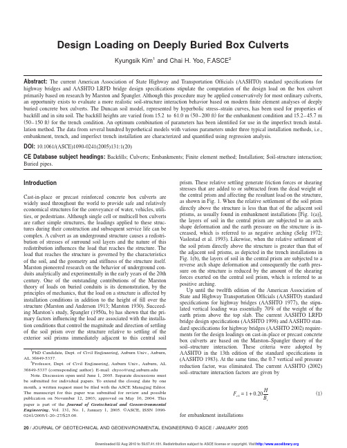
Design Loading on Deeply Buried Box CulvertsKyungsik Kim1and Chai H.Yoo,F.ASCE2Abstract:The current American Association of State Highway and Transportation Officials(AASHTO)standard specifications for highway bridges and AASHTO LRFD bridge design specifications stipulate the computation of the design load on the box culvert primarily based on research by Marston and Spangler.Although this procedure may be applied conservatively for most ordinary culverts, an opportunity exists to evaluate a more realistic soil-structure interaction behavior based on modernfinite element analyses of deeply buried concrete box culverts.The Duncan soil model,represented by hyperbolic stress–strain curves,has been used for properties of backfill and in situ soil.The backfill heights are varied from15.2to61.0m͑50–200ft͒for the embankment condition and15.2–45.7m ͑50–150ft͒for the trench condition.An optimum combination of parameters has been identified for use in the imperfect trench instal-lation method.The data from several hundred hypothetical models with various parameters under three typical installation methods,i.e., embankment,trench,and imperfect trench installation are characterized and quantified using regression analysis.DOI:10.1061/(ASCE)1090-0241(2005)131:1(20)CE Database subject headings:Backfills;Culverts;Embankments;Finite element method;Installation;Soil-structure interaction; Buried pipes.IntroductionCast-in-place or precast reinforced concrete box culverts are widely used throughout the world to provide safe and relatively economical structures for the conveyance of water,vehicles,utili-ties,or pedestrians.Although single cell or multicell box culverts are rather simple structures,the loadings applied to these struc-tures during their construction and subsequent service life can be complex.A culvert as an underground structure causes a redistri-bution of stresses of surround soil layers and the nature of this redistribution influences the load that reaches the structure.The load that reaches the structure is governed by the characteristics of the soil,and the geometry and stiffness of the structure itself. Marston pioneered research on the behavior of underground con-duits analytically and experimentally in the early years of the20th century.One of the outstanding contributions of the Marston theory of loads on buried conduits is its demonstration,by the principles of mechanics,that the load on a structure is affected by installation conditions in addition to the height offill over the structure(Marston and Anderson1913;Marston1930).Succeed-ing Marston’s study,Spangler(1950a,b)has shown that the pri-mary factors influencing the load are associated with the installa-tion conditions that control the magnitude and direction of settling of the soil prism over the structure relative to settling of the exterior soil prisms immediately adjacent to this central soil prism.These relative settling generate friction forces or shearing stresses that are added to or subtracted from the dead weight of the central prism and affecting the resultant load on the structure, as shown in Fig.1.When the relative settlement of the soil prism directly above the structure is less than that of the adjacent soil prisms,as usually found in embankment installations[Fig.1(a)], the layers of soil in the central prism are subjected to an arch shape deformation and the earth pressure on the structure is in-creased,which is referred to as negative arching(Selig1972; Vaslestad et al.1993).Likewise,when the relative settlement of the soil prism directly above the structure is greater than that of the adjacent soil prisms,as depicted in the trench installations in Fig.1(b),the layers of soil in the central prism are subjected to a reverse arch shape deformation and consequently the earth pres-sure on the structure is reduced by the amount of the shearing forces exerted on the central soil prism,which is referred to as positive arching.Up until the twelfth edition of the American Association of State and Highway Transportation Officials(AASHTO)standard specifications for highway bridges(AASHTO1977),the stipu-lated vertical loading was essentially70%of the weight of the earth prism above the top slab.The current AASHTO LRFD bridge design specifications(AASHTO1998)and AASHTO stan-dard specifications for highway bridges(AASHTO2002)require-ments for the design loadings on cast-in-place or precast concrete box culverts are based on the Marston–Spangler theory of the soil–structure interaction.These criteria were adopted by AASHTO in the13th edition of the standard specifications in (AASHTO1983).At the same time,the0.7vertical soil pressure reduction factor,was eliminated.The current AASHTO(2002) soil–structure interaction factors are given byF e1=1+0.20HB c͑1͒for embankment installations1PhD Candidate,Dept.of Civil Engineering,Auburn Univ.,Auburn,AL36849-5337.2Professor,Dept.of Civil Engineering,Auburn Univ.,Auburn,AL36849-5337(corresponding author).E-mail:chyoo@Note.Discussion open until June1,2005.Separate discussions mustbe submitted for individual papers.To extend the closing date by onemonth,a written request must befiled with the ASCE Managing Editor.The manuscript for this paper was submitted for review and possiblepublication on November12,2003;approved on May10,2004.Thispaper is part of the Journal of Geotechnical and GeoenvironmentalEngineering,V ol.131,No.1,January1,2005.©ASCE,ISSN1090-0241/2005/1-20–27/$25.00.20/JOURNAL OF GEOTECHNICAL AND GEOENVIRONMENTAL ENGINEERING©ASCE/JANUARY2005F e 2=C d B d2HB c͑2͒for trench installations where F e 1,F e 2=soil–structure interaction factor;H =backfill height;B c =width of the structure;C d =load coefficient for trench installation;and B d =horizontal width of trench.BackgroundIf the result of a soil–structure interaction analysis is to be real-istic and meaningful,it is important that the stress–strain charac-teristics of the soil be represented in a reasonable way.There are two general categories of stiffness and/or compressibility models for soils:(1)models based on constant confining pressure triaxial tests,and (2)models based on uniaxial strain confined compres-sion tests.Soil models in the first category usually incorporate a failure condition,whereas those in the second category do not,because the failure condition is not defined in the uniaxial tests.Examples of the first category are the Hardin model (Hardin 1971),the Duncan model (Duncan and Chang 1970),and the bilinear model (McVay and Selig 1981),while the overburden-dependent model (Katona et al.1976)falls into the second cat-egory.Since the Duncan model is capable of obtaining its com-pressibility parameters from the uniaxial compression test,it is the most general of the models in the first category.Duncan and Chang (1970)expanded the basic hyperbolic stress–strain rela-tionship for soil suggested by Kondner (1963)to derive the tan-gent modulus of elasticity and Poisson’s ratio as follows:E t =ͫ1−R f ͑1−sin ␾͒͑␴1−␴3͒2c cos ␾+2␴3sin ␾ͬ2Kp aͩ␴3p aͪn͑3͒␯t =G −F logͩ␴3p aͪͭ1−Kp aͩ␴3p aͪnͫd ͑␴1−␴3͒͑1−sin ␾͒2c cos ␾+2␴3sin ␾ͬͮ2͑4͒where R f =failure ratio;␴1,␴3=maximum and minimum principal stresses;K =modulus number;n =modulus exponent;c =cohesion intercept;␾=friction angle;G,F,d =Poisson’s ratio parameters;and p a =atmospheric pressure.An attempt to reduce the load on the structure led to the de-velopment of the imperfect trench method (sometimes called the induced trench method )of construction,where larger relative ver-tical displacements of the soil prism above the structure are in-duced by replacing some part of the fill with lightweight material.Baled straw,leaves,compressive soil,or expanded polystyrene blocks are examples of the types of lightweight material that can be used.It was intuitively expected that the result of this light-weight backfill was to introduce a reverse arch shape deforma-tion,causing a radical alteration of the culvert pressure distribu-tion due to the fill subsequently placed above the soft zone.Brown (1967)quantified the pressure reduction effect of the hay layers based on the finite element method of plane elasticity.Vaslestad et al.(1993)revisited this imperfect trench installation method to examine the long-term behavior of the load reduction characteristics on rigid culverts beneath high fills.Linear and nonlinear stress analyses in geotechnical engineer-ing for static and dynamic loading were introduced in the late 1960s and early 1970s.Kulhawy et al.(1969)developed LSBUILD ,a finite element program for stresses and movements in embankments during construction.In ISBILD ,an updated ver-sion of LSBUILD ,Ozawa and Duncan (1973)incorporated a non-linear incremental finite element procedure employing a hyper-bolic stress–strain relationship.Techniques for determining values of the hyperbolic parameter were later presented and updated (Wong and Duncan 1974;Duncan et al.1980).Allen and Meade (1984)used the program ISBILD to predict loads on and settle-ments of concrete culverts that had been actually installed in Ken-tucky.Their results indicated that the finite element method pre-dicted the pressure on box culverts more accurately than other analytical methods available at the time.Katona et al.(1976)developed CANDE ,which is a special-purpose finite element pro-gram primarily intended for the design and analysis of buried culverts.The CANDE program has been widely used for soil–structure analysis and evaluation of buried box culvert designs by a number of researchers,including Chang et al.(1980),Katona and Vittes (1982),and Tadros et al.(1989).CANDE has been upgraded several times,with the latest version being CANDE-89(Musser 1989).Most recently,Kim and Yoo (2002a,b )investi-gated load distributions on deeply buried concrete box culverts using the programs ISBILD and CANDE-89.Finite Element ModelIn the present study,ABAQUS (1998)and ISBILD were used pri-marily for the analysis and CANDE-89for verification and com-parison.The ISBILD code incorporates a nonlinear incremental finite element method employing the hyperbolic stress–strain re-lationship and incremental analysis procedures based on plane strain elements.As required ABAQUS inputs for the material properties of soils,the tangent modulus of elasticity and Poisson’s ratio,are evaluated for each construction layer using Eqs.(3)and (4).In order to quantify the maximum and minimum principal stresses that are needed in Eqs.(3)and (4),the following equa-tions are derived based on the assumption that soil layers are subjected to normal stresses without any induced shear stress:␴1͑i ͒=␥i ͑h i /2͒+͚j =i +1n␥j h j͑5͒Fig.1.Pressure transfer within soil-structure system:(a )embank-ment installation and (b )trench installationJOURNAL OF GEOTECHNICAL AND GEOENVIRONMENTAL ENGINEERING ©ASCE /JANUARY 2005/21␴3͑i ͒=R ␴1͑i ͒͑6͒where h i ,␥i =depth and density of the i th soil layer (numberingfrom the bottom to the top of the backfill,or original ground )and R ,the coefficient of lateral pressure,is taken to be 0.5in this study.Taking advantage of the symmetry,only one half of the struc-ture and the surrounding soil were modeled.Exactly the same geometric mesh,boundary conditions,and numbers of construc-tion layers were considered in both ABAQUS and ISBILD runs.It is expected that the width of the surrounding soil taken in the finite element model will affect the analysis results of soil-structure models.Soil–structure interaction factors or the effective densities (equivalent hydrostatic pressure )of the overburden soil increase as the ratio of the width of the soil layer ͑W s ͒to the width of the box culvert ͑B C ͒increases.Kim and Yoo (2002b )reported that the value of the soil–structure interaction factor in-crease gradually until W s /B c reaches approximately 12–14,after which no significant increase was observed.Therefore,W s /B c was taken to be 14in all subsequent analyses of soil–structure models.The width of the surrounding soil was taken to be six times the culvert width in the trench installations and the depth of the foundation below the bottom slab was taken to be four times the culvert height,as models based on a greater amount of in situ soil either vertically or horizontally did not affect the results.Typical soil–structure models with incremental sequences consid-ered for the embankment and trench installations are illustrated in Fig.2.Heights of backfill varied from 15.2m ͑50ft ͒to 61.0m ͑200ft ͒for the embankment installations,and from 15.2m ͑50ft ͒to 45.7m ͑150ft ͒for the trench installations.The constant exterior dimensions of the culvert were 2.4m ͑8ft ͒by 2.4m ͑8ft ͒,with 305mm ͑12in.͒thick walls and slabs.In cases where the height of the backfill exceeds 47.5m ͑150ft ͒,the thickness of walls and slabs may have to be increased to resist the induced shearing force near the wall face.It was found from a series of numerical analyses that the thickness of the culvert did not sig-nificantly alter the total load at the top of the culvert,having an effect only in the order of 1%.The modulus of elasticity of con-crete box culverts was computed to be 25,181MPa ͑3,605ksi ͒,assuming the 28day strength of concrete f c Јis 27.58MPa ͑4,000psi ͒and Poisson’s ratio ␯is 0.20.Hyperbolic parameters for the Duncan soil model were taken from Allen and Meade (1984).Effects of Soil–Structure Interface ModelingAn interface phenomenon that is frequently discussed is slip be-tween the soil and sidewalls of a culvert.Research has shown that there are basically two modeling techniques for the soil–structure interface examination,one of which is a shear element interface and the other a spring element (Katona et al.1976).Fig.3illus-trates the basic concept of these two modeling techniques.Table 1summarizes soil-structure interaction factors evaluated based on models with and without the effect of soil–structure interface.The hypothetical models examined in Table 1were assumed buried at a depth of 30.5m ͑100ft ͒.The dimensions of the box culvert are the same as those used for the comparative study presented here and other details such as the spring constant can be found in Kim and Yoo (2002b ).As can be seen from Table 1,the effect of a potential slip of the soil along the exterior culvert wall is insig-nificant.Therefore,the effect of interface action was not consid-ered in subsequent analyses.Comparison of Finite Element ModelingIn order to assess the validity of the soil modeling technique adopted in this study,an example used by Katona and Vittes (1982)was reanalyzed.The example is a single cell box culvert with interior dimensions of 1.22m ϫ1.22m and 254mm thick walls (4ft ϫ4ft and 10in.thick )tested in Kentucky in 1975.Pressure gage readings were taken at the backfill height of 6.6m ͑21.6ft ͒and 23.5m ͑77ft ͒.Fig.4shows the soil pressure around the box culvert predicted analytically by CANDE and ABAQUS .As can be seen from Fig.4,the analytically predicted values from ABAQUS are fairly close to those from CANDE .The analytically predicted soil pressure values are also fairly close to those deter-mined experimentally.The soil pressure directly above the side-Table parison of Soil–Structure Interaction Factors (SSIFs )SSIFDifferences a (%)Without interface 1.264—Spring model 1.2760.9Shear modelE S /E I bϭ101.277 1.0E S /E I bϭ201.288 1.9E S /E I bϭ501.310 3.6E S /E I bϭ1001.333 5.5E S /E I bϭ5001.3859.6aDifferences were computed based on the case without soil–structure interface.bE S /E I =ratio of the modulus of elasticity of soil to the fictitious shearelement.Fig.2.Incremental sequences:(a )embankment installation and (b )trenchinstallationFig.3.Interface modeling of culvert wall and soil elements:(a )shear element model and (b )spring element model22/JOURNAL OF GEOTECHNICAL AND GEOENVIRONMENTAL ENGINEERING ©ASCE /JANUARY 2005wall is substantially higher than the soil pressure at the center of the top slab,where the largest relative vertical deflection is ex-pected to occur.Embankment InstallationsThe pressure values on the topflange of the box culverts were averaged and conservatively converted to the effective densities or soil-structure interaction factors F e1and F e2,given by Eqs.(1) and(2).The effective density or the soil-structure interaction fac-tor is higher for an unyielding foundation than for a yielding foundation.Examination of the soil settlement adjacent to the culvert reveals that soil layers on an unyielding foundation[Fig. 5(b)]settle more at the level of the topflange than those on a yielding foundation[Fig.5(a)].As explained earlier and shown in Fig.1,the magnitude of relative settlements of soil prisms adja-cent to the central soil prism affects the effective soil density.Fig.6shows the effective density versus backfill height for culverts on yielding foundations.Effective densities increase as the backfill heights increase.The relative settlement of soil layers on a yielding foundation,illustrated in Fig.5,increases slightly more than linearly.Effective densities from ABAQUS are slightly higher than those from ISBILD.The predicted values from both ABAQUS and ISBILD lie between the values given for the com-pacted and the uncompacted side-fill by AASHTO(2002).Termi-nologies for compaction requirements in AASHTO such as“un-compacted”or“compacted,”used without quantitative references,are difficult to interpret in modern construction con-tracts.The compactness offill along the sides of the box section does not appear to significantly affect the effective density for deeply buried box culverts.It is clear that the effective density is most sensitive to the foundation characteristics.However,concrete box culverts are most likely to be installed on yielding foundations unless a solid rock layer is encountered immediately under the concrete box culverts.The AASHTO stipulates that a special analysis is re-quired for a culvert on an unyielding foundation.Fig.7shows the effective density versus backfill height for box culverts installed on unyielding foundations.The value of the effective density from ABAQUS showed somewhat higher values than those ob-tained from ISBILD.The following equations are proposed for the effective densities for yielding and unyielding foundations,re-spectively:D E=1.047H0.055;yielding foundation͑7͒D E=1.200H0.059;unyielding foundation͑8͒where DE and H stand for effective density andfilling height, respectively.While there are only small differences in the effec-tive densities determined from ABAQUS and ISBILD runs for yielding foundations,as shown in Fig.6,there are fairly large differences in the effective densities determined from ABAQUS and ISBILD for unyielding foundations,as shown in Fig.7.Eqs.Fig.5.Deformed shapes of soil layers adjacent to box culvert:(a) yielding foundation and(b)unyieldingfoundation Fig.6.Effective density for embankment installations on yieldingfoundations parison of soil pressure around box culvertTrench InstallationsThe pressure values on the top flange of the box culverts were averaged and conservatively converted to effective densities.The effect of sloping trench walls and vertical sidewalls was investi-gated.The effective density asymptotically approaches that for embankment installation as the ratio of the horizontal width of the trench to the box width ͑B d /B c ͒increases,as expected.The ef-fective density for vertical sidewalls is plotted as a function of the ratio of backfill height to horizontal width ͑H /B d ͒on yielding and unyielding foundations in Figs.8and 9,respectively.As in the case of embankment installation,the effective densities deter-mined from ABAQUS are slightly higher than those computed from ISBILD .Most values of the soil–structure interaction factor from AASHTO (2002)are 1.4,the upper limit value.It is clear from Fig.8that the effective density given by the current AASHTO is conservative compared to the analytically predicted values from this study.The curves shown are fitted from a regres-sion analysis on the data from ABAQUS and ISBILD as functions of H /B d .It is noted that different effective densities can be found for the same value of H /B d as the magnitude of the backfill height H may have a nonlinear effect on the effective density,as men-tioned earlier.It should also be noted that there are no effective densities plotted in Fig.9,as there are no procedures presented in the current AASHTO other than stipulating a special analysis re-quirement.Predictor equations for effective densities formulated from ABAQUS runs are proposed as follows:D E =exp ͓0.012͑H /B d ͒2−0.288͑H /B d ͒+0.375͔;yielding foundation͑9͒D E =exp ͓0.011͑H /B d ͒2−0.273͑H /B d ͒+0.465͔;unyielding foundation͑10͒In most theoretical treatments,the trench walls are generally taken to be vertical.However,for deep trenches,it is not practical to maintain the trench walls to be vertical.Sloping trench side-walls are expected to have a significant effect on the soil pressure on culverts.For cases where the trench is constructed with slop-ing walls,it is usual that the width of the trench B d is taken as the horizontal distance between the sloping walls at the top of the box.In order to investigate the effect of the sloping sidewalls on the effective density,a number of hypothetical concrete culverts installed in a trench with sloping sidewalls were analyzed.Fig.10shows the effective densities for trench installations with sloping sidewalls.It is believed that such quantified information on the effect of the sloping sidewall has not previously been available.The ranges of the parameters used to generate Fig.10were:ratio of the trench width to the concrete box culvert width B d /B c =2,3,4;and fill height H =15.2m ͑50ft ͒,30.5m ͑100ft ͒,45.7m ͑150ft ͒.␪represents the angle between the vertical line and the sloping sidewall of the trench.Effective densities increase to ap-proximately 90%of those for embankment installations when ␪approaches 45°.Although Fig.8shows large differences between the values of the effective density computed from AASHTO pro-visions and finite element analyses where the trench walls are assumed to be vertical,the actual differences are likely to be smaller when the sloping trench walls are taken into account.Imperfect Trench InstallationsThe loads on concrete box culverts in embankment installations are greater than the weight of the soil directly above the structure,as stated previously.An attempt to reduce the load on the struc-ture led to the development of the imperfect trench method of construction,as shown in Fig.11.As the embankment is con-structed,the soft zone compresses more than the surrounding fill and thus induces a reverse arch deformation above the culvert.Concrete box culverts buried with a lightweight material zone were analyzed for several different geometric configurations and backfill material properties.The modulus of elasticity of the light-Fig.7.Effective density for embankment installations on unyieldingfoundationsFig.8.Effective density versus H /B d for trench installations on yieldingfoundationsFig.9.Effective density versus H /B d for trench installations on unyielding foundations4.79kPa ͑10ksf ͒and the weight was taken to be 1.57kN/m 3͑10lb/ft 3͒.A typical average value of modulus of elasticity of soil E is about 10–20kPa at ground level and 200kPa at a depth of 30m.The width of the lightweight backfill or the loose mate-rial zone w was varied from 1to 2.5times the width of the culvertB c .The exterior dimensions of the box culvert were 2.44m ͑8ft ͒high and 2.44m ͑8ft ͒wide,and the thickness of the slab and wall were both 305mm ͑12in.͒.Table 2shows the load reduction rate of the imperfect trench method in terms of percentage for a concrete box culvert buried at a depth of 30.5m ͑100ft ͒with a lightweight material zone above 0.6m ͑2ft ͒from the top of the culvert.The height of the lightweight material zone was set at 2.44m ͑8ft ͒.Table 2clearly demonstrates that the width of the lightweight backfill zone need not be greater than 1.5times the width of the culvert,as no significant load reduction is realized beyond that.This number agrees well with the recommendation by Vaslestad et al.(1993).The effects of the height of the lightweight material zone h and the distance between the culvert and the lightweight material zone h Јwere also examined.h and h Јwere varied from 0.75m ͑2.5ft ͒to 4.5m ͑15ft ͒,and from 0to 2.44m ͑8ft ͒,respectively.The load reduction rates as functions of the ratio of the height of the soft zone to that of the culvert h /H c are plotted with different values of w /B c in Fig.12and with different moduli in Fig.13.It can be seen from Figs.12and 13that the ratio h /H c need not be greater than 1.5;after which no significant load reduction is real-ized.The variations of load reduction rates are shown in Fig.14as a function of the ratio of the distance between the culvert and the lightweight material zone to the height of the culvert h Ј/H c .Note that the maximum load reduction rate is realized if the light-weight backfill or the soft zone is placed immediately above the box culvert.However,it may be necessary to place a nominal layer of backfill over the box in order to facilitate the construction of the lightweight material zone.Typical effective density distri-butions on the box culverts are shown in Fig.15for different values of w /B c ,E ,and h Ј/H c .It is evident from Figs.12–15that the imperfect trench method can significantly reduce the effective densities or the soil–structure interaction factors.The notion of inducing artificial reverse arch shape deformations in the backfill above buried conduits,thereby reducing the vertical soil pressure,Fig.12.Effects of w /B c and h /H c in imperfect trench installationsFig.10.Effect of sloping sidewall in trench installationsFig.11.Concept and notation in imperfect trench installationsTable 2.Load Reduction Rates (%)Due to Imperfect Trench Installation Modulus of lightweight materialWidth of back fill layer,w /B c 1.0 1.5 2.0 2.547.9kPa ͑100ksf ͒32.841.139.136.723.9kPa ͑50ksf ͒43.658.657.054.34.79kPa ͑10ksf ͒56.983.785.384.8JOURNAL OF GEOTECHNICAL AND GEOENVIRONMENTAL ENGINEERING ©ASCE /JANUARY 2005/25has been known and tried intermittently (Brown 1967).It is be-lieved,however,that numerical values of the parameters for the optimum size of the lightweight material zone and its desired location have not been available elsewhere before this study.However,the imperfect trench method is an emerging technology that so far lacks a great deal of construction experience.Vaslestad et al.(1993)recommend a judicious selection of the lightweight backfill material and its careful installation,as many unsatisfac-tory experiences have been reported.Summary and Concluding RemarksLinear and nonlinear finite element analyses have been conducted to investigate the effective density or soil–structure interaction factor for deeply buried concrete box culverts.The effective den-sities are sensitively affected by many parameters,including in-stallation methods and foundation characteristics.Although con-servative classical methods will continue to be applied to the design and construction of buried conduits,an opportunity exists to utilize the modern numerical techniques made possible by ad-vances in finite element methods.The findings from this study presented in the form of proposed regression equations and charts should find their applicability.Highlights of the study are as fol-lows:1.Soil–structure interaction factors for deeply buried box cul-verts are more sensitively affected by the foundation charac-teristics.Predictor equations for soil–structure interaction factors were derived based on numerical data for culverts on both yielding and unyielding foundations constructed by em-bankment,trench,and imperfect trench installation methods.2.The effect of possible slips of the sidefill materials along the exterior culvert wall on the vertical soil pressure on the box culvert was found to be negligibly small.3.The current AASHTO provisions and most other references stipulate the effective densities for the trench installations under the assumption that the trench walls are excavated ver-tically.However,it was found that the effect of sloping trench walls on the soil–structure interface factors is very high.Fig.10presents variations of the soil–structure interac-tion factors as functions of major parameters,including the fill height,the degree of slope,and other trench geometry.4.Effective densities or the soil–structure interaction factors may be significantly reduced by properly implementing the imperfect trench method.Load reduction rates afforded by inducing artificial reverse arch shape deformations can be as high as 85%,depending on the dimensions of the lightweight material zone and the modulus of elasticity of the lightweight material.The height and the width of the lightweight mate-rial zone need not be greater than 1.5times those of the box culvert,beyond which no significant load reduction is real-ized.The greatest effect on load reduction is also obtained if the lightweight material zone can be placed immediately above the box culvert,although it may be necessary to place a nominal backfill layer immediately above the box to facili-tate the construction of the lightweight material zone.It is believed that the optimum values defining the lightweight material zone and its location have not been available else-where before this study.AcknowledgmentFunding for this research project was provided by the Highway Research Center,Auburn University.This financial support is gratefullyacknowledged.Fig.13.Effects of Young’s modulus and h /H c in imperfect trenchinstallationsFig.15.Effective density affected by imperfect trenchinstallationsFig.14.Effects of w /B c and h Ј/H c in imperfect trench installations26/JOURNAL OF GEOTECHNICAL AND GEOENVIRONMENTAL ENGINEERING ©ASCE /JANUARY 2005。

高产优质两系杂交稻新品种Y 两优919的综合评价任代胜,王思哲,杨家来,乔保建∗㊀(安徽袁粮水稻产业有限公司,安徽芜湖241003)摘要㊀旨在评价长江中下游稻区新选育的中籼迟熟新品种Y 两优919,满足市场对水稻新品种的需求㊂基于2018 2019年长江中下游稻区新选育的中籼迟熟新品种的区试与生产试验数据,利用相关性㊁主成分(PCA )与偏最小二乘判别分析方法(PLS -DA ),综合评价Y 两优919的农艺经济性状㊁主要病虫害抗性与品质㊂结果表明,与对照品种丰两优4号相比,Y 两优919两年产量均显著提高,增幅分别达到8.03%和8.14%;同时2年各区试点产量变异系数较低,分别为1.61%和2.41%,表现出较好的丰产性与稳产性;Y 两优919的病虫害抗性均优于各区试点对照品种,其米质更是达到部颁三等优质稻标准㊂此外,相关性㊁PCA 与PLS -DA 分析结果表明,产量为丰两优4号与Y 两优919的关键差异性状㊂综上可知,Y 两优919农艺经济性状㊁主要病虫害抗性与品质等综合表现优良,应进一步示范试验和推广应用㊂关键词㊀两系杂交中籼稻;相关性分析;主成分分析;偏最小二乘判别分析中图分类号㊀S 511㊀㊀文献标识码㊀A㊀㊀文章编号㊀0517-6611(2023)21-0023-06doi :10.3969/j.issn.0517-6611.2023.21.007㊀㊀㊀㊀㊀开放科学(资源服务)标识码(OSID):Comprehensive Evaluation of the Newly Two-line Hybrid Rice Variety Y-liangyou 919with High-yield and Fine-quality REN Dai-sheng ,WANG Si-zhe ,YANG Jia-lai et al㊀(Anhui Yielead Rice Industry Co.,Ltd.,Wuhu,Anhui 241003)Abstract ㊀The aim is to evaluate the newly selected new medium Indica late-maturing variety Y-liangyou 919in the middle and lower reaches of Yangtze River rice region to meet the market demand for new rice varieties.Based on data from regional and production trials of newly se-lected new medium Indica late-maturing varieties in the middle and lower reaches of the Yangtze River rice region in 2018and 2019,the cor-relation,principal component (PCA)and partial least squares discriminant analysis (PLS-DA)methods were applied to comprehensively e-valuate the agronomic and economic traits,major pest and disease resistance and quality of Y-liangyou 919.The results showed that compared with the control variety Fengliangyou 4,the yields of Y-liangyou 919were significantly higher in both years,with increment of 8.03%and 8.14%,respectively.Meanwhile,its yield coefficients of variation were low in both years,1.61%and 2.41%in each pilot zone,respective-ly,showing better yield and stability.Importantly,the pest and disease resistance of Y-liangyou 919was better than that of the control variety in each district pilot,and its rice quality even reached the third grade quality rice standard of the Ministry.In addition,the results of correla-tion,PCA and PLS-DA analyses showed that yield was the key differential trait between Fengliangyou 4and Y-liangyou 919.Above all,it could be concluded that Y-liangyou 919had excellent agronomic and economic traits,major pest and disease resistance and quality,and should be further demonstrated and applied.Key words ㊀Two-line hybrid rice;Correlation analysis;Principal component analysis;Partial least-squares discriminant analysis基金项目㊀安徽省重点研究与开发计划面上攻关-农业领域项目(202104a06020039)㊂作者简介㊀任代胜(1989 ),男,安徽广德人,农艺师,硕士,从事水稻遗传育种研究㊂∗通信作者,副研究员,博士,从事高产优质杂交稻育种研究㊂收稿日期㊀2022-10-21㊀㊀水稻杂交是第二次绿色革命的首选技术,杂交水稻更关系到我国粮食与种业安全[1-2]㊂2015年新‘种子法“的施行更推进杂交水稻种子产业的振兴与产权保护[3]㊂水稻品种从选育到推广离不开区域试验,长江中下游地区历来是我国水稻主要产出地,籼稻种植面积和总产量约占全国50%,安徽省是我国主要的水稻生产区域,水稻常年播种面积247万hm 2,占全国水稻种植面积的8.5%[4]㊂在长江中下游地区进行品种选育,从丰产性㊁稳产性㊁抗病虫性和稻米品质等方面鉴定和评价新品种,既可为水稻品种的国家审定提供科学依据,也为新品种推广提供理论依据[5-6]㊂安徽袁粮水稻产业有限公司自主选育的两系杂交中籼水稻品种Y 两优919,其不育系Y58S 广适性水稻光温敏[7-8];恢复系R919是2012年安徽袁粮水稻产业有限公司利用R17/R9311//R425进行杂交㊁复交,选择抗倒伏㊁抗病㊁早熟㊁优质株系自交纯和育成㊂Y 两优919是安徽袁粮水稻产业有限公司在2016年冬在三亚配组而成,经2016 2017年多点测试,综合表现优良,定名为Y 两优919㊂鉴于此,笔者根据Y 两优919在2018 2019年长江中下游稻区多点区试产量和抗性的表现,利用相关性分析㊁主成分(principal component analysis,PCA)与偏最小二乘判别分析方法(partial least -squares discrimi-nant analysis,PLS -DA)综合评价中籼稻Y 两优919的农艺经济性状㊁主要病虫害抗性与稻米品质,为该水稻产区品种选用与推广应用提供理论依据㊂1㊀材料与方法1.1㊀试验材料与区试点㊀供试水稻品种Y 两优919(YLY919),以丰两优4号(FLY4)为对照品种㊂采用2018 2019年在14个长江中下游稻区区试点鉴定结果,试验点具体经纬度和海拔见表1㊂1.2㊀试验设计与方法㊀各区试点大田试验小区面积均为0.0013hm 2,3次重复,各小区采用完全随机区组设计㊂同时,各区试点采用与当地大田生产相同的栽培管理措施㊂1.3㊀指标检测1.3.1㊀产量与主要农艺性状㊂指标测定方法参照‘国家水稻品种试验观察记载项目㊁方法及标准“㊂1.3.2㊀主要病虫害抗性鉴定㊂根据病虫害抗性鉴定单位的结果报告为主要依据,即以水稻穗瘟发病率(%)与损失率(%)为依据评价稻瘟病抗性[9]㊂同时,白叶枯病与褐飞虱抗性的主要评价指标为最高级㊂1.3.3㊀稻米品质评价㊂品质评价依照农业行业标准NY /T安徽农业科学,J.Anhui Agric.Sci.2023,51(21):23-28㊀㊀㊀593 2013‘食用稻品种品质“进行,具体级别分别为优质1㊁2与3级,未达优质级则为普通级㊂表1㊀长江中下游区试试验点基本情况Table1㊀Basic information of the pilot sites in the middle and lower reaches of Yangtze River编号Number承试单位Undertakingorganization试验地点Test site经度Longitude(E)纬度Latitude(N)1安徽滁州市农业科学研究所滁州市国家农作物区域试验站118ʎ26ᶄ32ʎ09ᶄ2安徽黄山市种子站黄山市农科所双桥基地118ʎ14ᶄ29ʎ40ᶄ3安徽省农业科学院水稻研究所合肥市117ʎ32ʎ4安徽袁粮水稻产业有限公司芜湖市镜湖区利民村试验基地118ʎ27ᶄ31ʎ14ᶄ5河南信阳市农业科学研究院信阳市本院试验田114ʎ05ᶄ32ʎ07ᶄ6湖北京山县农业科学研究所京山县永兴镇苏佘畈村五组113ʎ07ᶄ31ʎ01ᶄ7湖北宜昌市农业科学研究院枝江市问安镇四岗试验基地111ʎ05ᶄ30ʎ34ᶄ8湖南怀化市农业科学研究所怀化市洪江市双溪镇大马村109ʎ51ᶄ27ʎ15ᶄ9湖南岳阳市农业科学研究所岳阳县麻塘试验基地113ʎ05ᶄ29ʎ24ᶄ10江苏里下河地区农业科学研究所扬州市119ʎ25ᶄ32ʎ25ᶄ11江苏沿海地区农业科学研究所盐城市120ʎ08ᶄ33ʎ23ᶄ12江西九江市农业科学研究所九江县马回岭镇115ʎ48ᶄ29ʎ26ᶄ13江西省农业科学研究院水稻研究所高安市鄱阳湖生态区现代农业科技示范基地115ʎ22ᶄ28ʎ25ᶄ14中国水稻研究所杭州市富阳区120ʎ19ᶄ30ʎ12ᶄ1.4㊀数据统计㊀利用Microsoft Excel2010收集整理统计数据㊂产量及主要农艺性状利用GraphPad Prism8.3作T-Test 差异显著性检验分析并绘图,利用变异系数(coefficient of variation,CV)评价品种稳产性和适应性㊂关键差异指标的PCA㊁PLS-DA分析与相关性热图绘制通过在线网站Metabo-Analyst5.0进行㊂2㊀结果与分析2.1㊀区试产量与主要农艺性状㊀2018年国家水稻品种区试与2019年生产试验结果显示,与丰两优4号相比,Y两优919的14个试验点的产量与主要农艺性状(千粒重与株高除外)均显著提高(图1)㊂Y两优919的产量分别为9895.80和10311.75kg/hm2,增幅达到8.03%与8.14%(图1b);每穗总粒数分别为193.8和201.4粒,增幅均达到5.09%(图1c);有效穗数分别为256.5万和250.5万/hm2,增幅达到11.50%和8.24%(图1d);每穗实粒数分别为193.80与180.44粒,增幅达到1.78%和11.38%(图1f);穗长均为27.7cm,增幅分别达到8.42%与8.03%(图1i)㊂此外,Y两优919的平均全生育期分别为137.5与139.2d,比丰两优4号分别迟熟4.3与4.2d(图1j)㊂2.2㊀主要病虫害抗性鉴定㊀2018年各试点水稻稻瘟病发病率与损失率结果可知(图2),与丰两优4号和各试点感稻瘟病品种CK相比,Y两优919的发病率与损失率均较低㊂根据综合评价结果可知(表2),丰两优4号的稻瘟病平均综合指数达到6.6级,穗瘟病损失率最高级为9级,属于高感稻瘟病品种;白叶枯病5级,属于中感白叶枯病品种;褐飞虱9级,属于高感褐飞虱品种㊂此外,Y两优919的稻瘟病平均综合指数则为5.0级,穗瘟损失率最高级为7级,属于感稻瘟病品种;白叶枯病5级,属于中感白叶枯病品种;褐飞虱9级,属于高感褐飞虱品种㊂㊀㊀2019年各试点结果可知(图2),与丰两优4号和各试点感稻瘟病品种CK相比,Y两优919的发病率与损失率较低㊂综合评价结果可知(表2),丰两优4号的稻瘟病平均综合指数7.5级,穗瘟损失率最高级9级,属于高感稻瘟病品种;白叶枯病5级,属于中感白叶枯病品种;褐飞虱9级,属于高感褐飞虱品种㊂Y两优919的稻瘟病平均综合指数4.6级,穗瘟损失率最高级7级,属于感稻瘟病品种;白叶枯病5级,属于中感白叶枯病品种;褐飞虱9级,属于高感褐飞虱品种㊂2.3㊀稻米品质分析㊀2018㊁2019年米质检测分析结果可知(表3),丰两优4号的糙米率分别为81.80%和80.90%,精米率分别为73.10%和73.60%,整精米率分别为59.00%与65.20%,粒长分别为6.90和6.70mm,长宽比均为3.10,垩白粒率分别为12%和25%,垩白度分别为1.60和2.20,透明度分别为1和2级,碱消值分别为6.2和6.5级,胶稠度分别为73与75mm,直链淀粉含量分别为15.10%和15.70%,综合评级为优质二级㊂Y两优919在2018㊁2019年的糙米率分别为81.60%和80.30%,精米率分别为73.50%和73.40%,整精米率分别为68.80%和70.30%,粒长分别为6.60和6.30mm,长宽比均为3.00,垩白粒率分别为5%和7%,垩白度分别为0.40%和0.60%,透明度均为2级,碱消值分别为5.3和5.0级,胶稠度分别为77和78mm,直链淀粉含量分别为13.30%和13.80%,综合评级为优质三级㊂2.4㊀产量成因性状分析㊀为进一步分析2个品种的产量与主要农艺经济性状的关系,以测定指标为自变量进行相关性㊁PCA与OPLS-DA分析㊂产量与农艺经济性状的相关性热图可知,产量与穗长㊁穗总粒数㊁穗实粒数与有效穗数间显著正相关(图3a)㊂进一步对所有农艺经济性状指标进行分类排序,相关性越强与产量越靠近,其直方柱状越长㊂由图3b可知,产量相关性由强到弱依次为穗长㊁穗实粒数㊁有效穗数㊁穗总粒数㊁全生育期㊁千粒重㊁结实率和株高㊂为更好地可视化丰两优4号与Y两优919的农艺经济性状差异,同时以测定指标为自变量进行PCA和PLS-DA 分析,以确定2个品种的关键差异性状㊂此外农艺性状的42㊀㊀㊀㊀㊀㊀㊀㊀㊀㊀安徽农业科学㊀㊀㊀㊀㊀㊀㊀㊀㊀㊀㊀㊀㊀㊀㊀㊀㊀㊀㊀㊀㊀㊀㊀㊀㊀2023年VIP 值(variable importance in projection)>1.0可作为品种关键差异性状㊂PCA 分析结果(图3c)可知,所有测定指标降维为5个主成分,其百分比分别为70.2%㊁25.3%㊁2.2%㊁1.2%和0.9%㊂同时,PLS -DA 分析(图3d)变量1和2可以很好地表征所有性状95.5%的信息,并将2个品种的农艺经济性状进行分组㊂进一步,对PLS -DA 分析中的成分1与2进行VIP 得分图可视化,以筛选区分2个品种差异的指标,同时验证品种的差异表型㊂从图3e 与3f 可以看出,产量是形成2品种分组的关键因素㊂注:∗表示2个品种间在0.05水平差异显著;∗∗表示2个品种间在0.01水平差异极显著;ns 表示2个品种间无显著差异(P ȡ0.05)㊂Note:∗indicated significant difference between two varieties (P <0.05),∗∗indicated highly significant difference between two varieties (P <0.01),and ns indicated no significant difference between two varieties (P ȡ0.05).图1㊀2018和2019年2个品种各试点的产量㊁构成因素与农艺性状比较Fig.1㊀Comparison of yield ,component factors and agronomic traits for each pilot of the two varieties in 2018and 20195251卷21期㊀㊀㊀㊀㊀㊀㊀㊀㊀㊀㊀㊀㊀㊀任代胜等㊀高产优质两系杂交稻新品种Y 两优919的综合评价注:感稻瘟病CK 在浙江㊁安徽均为Wh26,在湖南㊁湖北㊁福建㊁江西分别为湘晚籼11号㊁丰两优香1号㊁明恢86+龙黑糯2号㊁恩糯㊂Note:As forice plague-sensitive varieties (CK),Wh26was used in Zhejiang and Anhui;Xiangwanshan 11,Fengliangyouxiang 1,Minghui 86+Long-heinuo 2,Ennuo were used in Hunan,Hubei,Fujian and Jiangxi,respectively.图2㊀2018和2019年不同品种各试点稻瘟病抗性鉴定Fig.2㊀Identification of rice blast resistance in different varieties for each pilot in 2018and 2019表2㊀不同品种对主要病虫抗性综合评价Table 2㊀Comprehensive evaluation of the resistance of different varieties to major diseases and insects年份Year品种名称Variety name稻瘟病Rice blastʊ级浙江Zhejiang 湖南Hunan 湖北Hubei 安徽Anhui 福建Fujian 江西Jiangxi 平均综合指数Average composite index 损失率最高级The highest loss rate 抗性水平Resistance level 白叶枯病Rice bacterial blightʊ级平均综合指数Average composite index 抗性水平Resistance level 褐飞虱Brown rice planthopperʊ级平均综合指数Averagecompositeindex抗性水平Resistancelevel2018丰两优4号6.3 6.3 6.3 6.58.5 6.0 6.69HS 5MS 9HSY 两优919 2.8 4.5 4.5 5.87.3 5.3 5.07S 5MS 9HS CK17.58.88.58.58.58.58.49HS 9HS 9HS2019丰两优4号6.37.38.5 6.58.38.07.59HS 5MS 9HSY 两优919 4.8 6.0 2.5 4.3 3.5 4.5 4.67S 5MS 9HS CK27.59.08.58.88.58.58.59HS 9HS 9HS㊀注:CK1与CK2分别为金刚30(感白叶枯病)和TN1(褐飞虱); MS 为中感㊁ S 为感㊁ HS 为高感㊂㊀Note:CK1and CK2were Jingang 30(susceptible to white leaf blight)and TN1(brown fly),respectively;MS was moderately susceptible,S was susceptibleand HS was highly susceptible.表3㊀稻米品质评价结果Table 3㊀The results of rice quality evaluation品种名称Variety name 年份Year 糙米率Rough rice rate%精米率Fine rice rate %整精米率Whole fine rice rateʊ%粒长Grain length mm长宽比Aspect ratio 垩白粒率Chalk rateʊ%垩白度Chalkiness%透明度Transp-arency级碱消值Alkali depletion valueʊ级胶稠度Gum consistency mm 直链淀粉Straight chain starchʊ%综合评级Comph-rehensive standard丰两优4号201881.8073.1059.00 6.90 3.1012 1.601 6.27315.10优质二级Fengliangyou 4201980.9073.6065.20 6.70 3.1025 2.202 6.57515.70优质二级Y 两优919201881.6073.5068.80 6.60 3.0050.402 5.37713.30优质三级Y-liangyou 919201980.3073.4070.306.30 3.0070.6025.07813.80优质三级62㊀㊀㊀㊀㊀㊀㊀㊀㊀㊀安徽农业科学㊀㊀㊀㊀㊀㊀㊀㊀㊀㊀㊀㊀㊀㊀㊀㊀㊀㊀㊀㊀㊀㊀㊀㊀㊀2023年注:红㊁绿与黑色分别表示正㊁负与无相关性,其颜色越深则相关性越强㊂Note:Red,green and black indicate positive,negative and no correlation respectively;the darker the color the stronger the correlation.图3㊀不同品种各试点各指标的相关性㊁PCA与PLS-DAFig.3㊀The correlation,PCA and PLS-DA of each index for each pilot of different species3㊀结论与讨论多点区试和生产试验是选育和推广水稻新品种的基本流程,基于此新品种在不同水稻种植区的丰产性㊁稳产性和适应性可以最直观地展现[10-11]㊂试验期间,各区试点地理环7251卷21期㊀㊀㊀㊀㊀㊀㊀㊀㊀㊀㊀㊀㊀㊀任代胜等㊀高产优质两系杂交稻新品种Y两优919的综合评价境与气候条件的差异㊁人工统计误差等,都会造成新品种鉴定与评价的不客观[12]㊂因此,该研究对Y两优919的2018年区域试验和2019年生产试验的产量与主要农艺经济形状㊁病虫害抗性和稻米品质进行综合分析,进一步明确该品种特性㊂周健等[12]研究表明,水稻产量与其异地环境的生态适应性高度相关;李杰等[13]研究表明不同区域的栽培方式显著影响不同类型品种水稻产量及其农艺性状㊂此外,结合变异系数分析产量与农艺经济性状更能直接衡量新品种的稳定性与适应性[14-15]㊂该研究试验材料Y两优919的产量㊁每穗总粒数㊁每穗实粒数㊁有效穗数和穗长均显著高于对照品种,同时这些形状指标的变异系数均小于5%,表明Y两优919具有较好的丰产与稳产潜力;此外,PCA与PLS-DA分析结果表明,产量是Y两优919与对照品种的关键差异特性㊂然而,PCA分析结果可知,2个品种的产量与千粒重呈负相关,这是由于有效穗数㊁每穗实粒数和千粒重三者相互协调决定水稻产量,而Y两优919的有效穗数和每穗实粒数显著提高,表现其较优的品种特性[16]㊂此外,主要病虫害抗性中稻瘟病抗性鉴定评价最为严格,其抗性强弱以苗叶瘟㊁穗瘟发病率和穗瘟损失率病级进行加权统计形成的综合指数进行比较[6,9]㊂一般情况下,穗瘟导致水稻减产较为严重,穗瘟损失率与产量呈显著正相关,因此,综合指数和穗瘟损失率同时达标才符合国家审定标准[9,17]㊂Y两优919区域试验和生产试验的综合指数与穗瘟损失率均低于对照品种,说明其稻瘟病抗性基本达到国审标准㊂此外,稻米品质作为水稻的综合性状,已经成为现今水稻育种重要方向[18-19],因此现行稻米品质行业标准‘食用稻品种品质“(NY/T593 2013)要求更为严格[20]㊂该研究Y两优919具有较好的垩白度与直链淀粉含量,综合达到部颁优质三级标准㊂综上,Y两优919具有较好的丰产性与稳产性,稻瘟病抗性和主要农艺经济性状等综合表现优于对照品种,表现出较强的生态环境适应性,达到国家审定标准,具有市场推广潜力㊂参考文献[1]邹江石,吕川根.水稻超高产育种的实践与思考[J].作物学报,2005,31(2):254-258.[2]袁隆平.发展超级杂交水稻保障国家粮食安全[J].杂交水稻,2015,30(3):1-2.[3]邓光联.法律保障支撑推动种业发展:学习新修订‘种子法“的体会[J].中国种业,2016(2):1-7.[4]刘书通,李春生,方福平,等.长江中下游中籼杂交稻区试品种产量成因性状分析[J].中国农学通报,2015,31(15):7-11.[5]程本义,杨仕华,励立庆,等.中国长江流域新育成籼稻品种分析及育种应用[J].中国农学通报,2004,20(2):92-96.[6]林海,李红英,鄂志国,等.2020年我国审定的水稻品种基本特性分析[J].中国稻米,2021,27(6):6-11.[7]邓启云.广适性水稻光温敏不育系Y58S的选育[J].杂交水稻,2005,20(2):15-18.[8]吴俊,邓启云,袁定阳,等.超级杂交稻研究进展[J].科学通报,2016,61(35):3787-3796.[9]郝中娜,毛雪琴,柴荣耀,等.国家长江中下游稻区品种区域试验籼稻稻瘟病抗性分析[J].中国水稻科学,2019,33(2):152-157.[10]潘高峰,房振兵,田永宏,等.基于GGE双标图评价湖北省2017年中稻区试的品种和试点[J].湖北农业科学,2018,57(15):24-27. [11]廖留英,王洪飞,丁信良,等.早籼两系杂交水稻新品种聚两优919丰产稳产性分析与综合评价[J].现代农业科技,2022(8):11-14,17. [12]周健,崔迪,赵洙敏,等.不同年代水稻品种主要农艺性状的表型评价[J].植物遗传资源学报,2019,20(6):1566-1578.[13]李杰,张洪程,董洋阳,等.不同生态区栽培方式对水稻产量㊁生育期及温光利用的影响[J].中国农业科学,2011,44(13):2661-2672. [14]李忠芳,娄翼来,李慧,等.长期施肥下我国南方不同轮作制度水稻的高产稳产性分析[J].土壤,2015,47(5):830-835.[15]王鹤璎,郭晓红,张钦明,等.水条播对寒地水稻农艺性状和产量构成因素的影响[J].作物杂志,2020(1):81-88.[16]翟来圆,王峰,闫安,等.水稻穗粒数基因GNP1对库㊁源㊁流的生理机制剖析[C]//第十九届中国作物学会学术年会论文摘要集.北京:中国作物学会,2020:216.[17]李智谋,姜守全,于江辉,等.三系杂交稻稻瘟病抗性与产量的配合力分析[J].热带农业科学,2022,42(3):24-31.[18]卢朝军,周佳民,黄敏,等.长江中下游中籼迟熟水稻新品种稻米品质性状的主成分及聚类分析[J].现代农业科技,2008(5):136-138. [19]阙补超,孙滨,张伟,等.辽宁省中晚熟水稻新品种食味与品质性状的关系[J].中国农学通报,2013,29(33):379-382.[20]中华人民共和国农业部.中华人民共和国农业行业标准食用稻品种品质:NY/T593 2013[S].北京:中国标准出版社,2013.82㊀㊀㊀㊀㊀㊀㊀㊀㊀㊀安徽农业科学㊀㊀㊀㊀㊀㊀㊀㊀㊀㊀㊀㊀㊀㊀㊀㊀㊀㊀㊀㊀㊀㊀㊀㊀㊀2023年。

RICE2010模型一、模型描述RICE模型（区域气候和经济的综合模型）是从经济增长理论的框架上看待气候变化。

在一个被称为拉姆齐模型的标准新古典主义的最优增长模型中，社会在资本商品投资，减少现在的消费，来增加未来的消费。

RICE模型修改拉姆齐模型来包括气候投资。

常规模型的资本存量的被扩展到包括环境中的投资（“自然资本”）。

在扩展模型中减排类似于主流机型中的资本投资。

也就是说，我们可以把温室气体浓度看成“负自然资本”，减排看作负资本数量的减少。

通过致力于减排，降低现在的消费，防止经济上有害的气候变化，从而提高未来消费的可能性。

模型把世界分为12个区域。

有些是大的国家，如美国和中国；其他的是大的区域，如欧盟和拉美。

每个区域都假定有一个社会福利函数，随着时间的推移，每个区域都最优化它的消费量，温室气体的政策，以及投资。

在社会福利函数中消费边际效用递减，每一代人的人均消费增加。

一代人人均消费的重要性取决于人口规模。

不同代际的相对重要性受两个中央规范参数影响：纯时间偏好率和消费的边际效用弹性。

这两个参数相互作用决定了商品的折现率，这对跨经济选择是至关重要的。

在建模中，我们设置这些参数与观察到的经济成果是一致的，通过利率和资本回报率反映。

经济部门：假定每个区域只产生一个单一的商品，可以用于消费，投资，或减排。

每个区域被赋予了一个初始的资本存量和劳动力以及初始的技术水平。

人口数据来自联合国，更新的最新估计到2009年，采用联合国预测的2300年数据。

产出按恒定价格计算国内生产总值，不同国家的GDP转换成定值美元。

采用购买力平价汇率（PPP）计算的国际价格。

产出数据来自2009年世界银行和国际货币基金（IMF）的数据，从国际货币基金组织（IMF）得到直到2014年的预测。

直到2008年的二氧化碳的排放量数据来自美国能源情报署和二氧化碳信息分析中心。

人口增长和技术变革是特定区域和外生的，而资本积累是通过优化消费确定的。

作物学报ACTA AGRONOMICA SINICA 2024, 50(1): 126 137 / ISSN 0496-3490; CN 11-1809/S; CODEN TSHPA9E-mail:***************DOI: 10.3724/SP.J.1006.2024.34045棉花AP2/ERF转录因子GhTINY2负调控植株抗盐性的功能分析肖胜华1,2,**,*陆妍1,**李安子1覃耀斌1廖铭静1闭兆福1卓柑锋1朱永红2朱龙付2,*1 广西大学农学院 / 亚热带农业生物资源保护与利用国家重点实验室, 广西南宁 530000; 2华中农业大学 / 作物遗传改良国家重点实验室, 湖北武汉 430000摘要: 棉花属于相对耐盐作物, 但高盐胁迫同样会造成棉花产量和纤维品质的大幅下降。

深入挖掘抗盐基因并解析棉花响应盐胁迫的分子机理, 对加快棉花抗盐遗传改良育种进程具有重要意义。

本研究从棉花响应盐胁迫的转录组数据中鉴定到一个受盐诱导极显著下调表达的AP2/ERF转录因子GhTINY2, 并分析了GhTINY2超表达拟南芥的抗盐表型和各生理指标。

结果显示, 在盐胁迫下, GhTINY2超表达植株的种子萌发率显著下降; 脯氨酸、可溶性糖、叶绿素含量等均显著减少; 多个盐胁迫响应基因显著下调表达; 因而表现出更为严重的叶片萎蔫枯黄表型。

通过分析GhTINY2超表达拟南芥中的RNA-seq数据, 发现差异表达基因(DEGs)富集到叶绿素代谢、刺激响应等生物过程中,且DEGs均呈下调表达趋势。

此外, 在棉花中通过病毒诱导的基因沉默(VIGS)试验沉默GhTINY2后, TRV:GhTINY2植株在盐胁迫下叶绿素和脯氨酸含量显著增加, 从而增强了棉花的抗盐性。

综上, GhTINY2是棉花中一个负调控盐胁迫抗性的重要基因, 未来将有望通过现代基因工程技术利用GhTINY2创制耐盐棉花材料。

关键词:棉花; GhTINY2; 盐胁迫; 转录因子; 转基因Function analysis of an AP2/ERF transcription factor GhTINY2 in cotton nega-tively regulating salt toleranceXIAO Sheng-Hua1,2,**,*, LU Yan1,**, LI An-Zi1, QIN Yao-Bin1, LIAO Ming-Jing1, BI Zhao-Fu1, ZHUOGan-Feng1, ZHU Yong-Hong2, and ZHU Long-Fu2,*1 State Key Laboratory of Conservation and Utilization of Agro-Biological Resources in Subtropical Region / College of Agriculture, Guangxi Uni-versity, Nanning 530000, Guangxi, China; 2 State Key Laboratory of Crop Genetic Improvement, Huazhong Agricultural University, Wuhan 430000,Hubei, ChinaAbstract: Cotton is a relatively salt-tolerant crop, but high salt stress leads to a significant decline in cotton yield and fiber quality.Mining the genes involved in salt-tolerance and illuminating the molecular mechanisms that underlie this resistance is of greatimportance in cotton breeding programs. Here, we identified an AP2/ERF transcription factor GhTINY2 in the transcriptome da-tabase from cotton treated with salt, and the relative expression level of GhTINY2 was reduced by salt. Subsequently, thesalt-resistant phenotype and physiological indicators of the GhTINY2-overexpression Arabidopsis were analyzed. The resultsrevealed that the GhTINY2-overexpression Arabidopsis had a significant decrease in seed germination rate, the content ofproline, soluble sugar, and chlorophyll under salt stress, leading to more severe leaf wilting compared with WT. RNA-seq datafrom GhTINY2-transgenic Arabidopsis revealed that differentially expressed genes (DEGs) were enriched in a series of bio-logical processes, including chlorophyll metabolism and response to stimulus, and the relative expression level of these DEGs本研究由广西大学高层次人才科研启动基金项目(A3310051044)和广西大学农学院科研发展金项目(EE101711)资助。

色谱long term stability 定义Long term stability of chromatography is a crucial factor for ensuring consistent results in the analysis of biomolecules and for reliable applications in clinical and research settings.By definition, chromatography long term stability is the ability to maintain high-performance results, over time. That is, the ability of the chromatographic system to maintain precise and reproducible separations on a daily basis over a course of months or years. It is a quality indicator that measures the degree of variance in the individual components of the chromatographic system over a long period of time.High-resolution chromatographic separations require precise control of pressure, temperature, flow rate, mobile phase composition and detector parameters. Long term stability is strongly affected by factors such as instrument maintenance and calibration, column aging, particle stability, solvent evaporation and slowing, and any other external influences. The stability of the chromatographic system must be regularly monitored in order to ensure that it remains consistently stable.The stability of the chromatography system can be evaluated both experimentally and computationally. Experimentally, chromatographic results are subjected to a wide range of experiments and tests in order to determine the extent of the system's stability. Computer simulations are also employed to understand how different components of the system may interact with one another and how they affect the performance of the system.In summary, long term stability of chromatographic systems is an important indicator of a system's quality. It is a measure of overall system performance and helps to ensure that reliably accurate and reproducible results are obtained. Proper maintenance and calibration of the system is essential for ensuring superior long term stability.。

A race to the bottom?Employment protection and foreign direct investment ☆William W.OlneyDepartment of Economics,Williams College,Williamstown,MA 01267,United Statesa b s t r a c ta r t i c l e i n f o Article history:Received 31July 2012Received in revised form 1August 2013Accepted 21August 2013Available online 16September 2013JEL classi fication:F16F23J80Keywords:Foreign direct investment Employment protection Race to the bottomA common critique of globalization is that it leads to a race to the bottom.Speci fically,it is assumed that multi-nationals invest in countries with lower regulatory standards and that countries competitively undercut each other's standards in order to attract foreign capital.This paper tests this hypothesis and finds robust empirical support for both predictions.First,a reduction in employment protection rules leads to an increase in foreign direct investment (FDI).Furthermore,changes in employment protection legislation have a larger impact on the relatively mobile types of FDI.Second,there is evidence that countries are competitively undercutting each other's labor market standards.©2013Elsevier B.V.All rights reserved.1.IntroductionA frequent critique of globalization is that it can lead to a race to the bottom,where countries lower their labor standards,environmental stan-dards,or tax rates in order to attract foreign capital.1More speci fically,the race to the bottom hypothesis hinges on two important predictions.First,multinational enterprises (MNE)choose to invest in countries with less restrictive standards.Second,foreign countries competitively undercut each other's standards in order to attract foreign direct investment (FDI).While these are common fears associated with globalization,there is relatively little empirical evidence supporting either of these pre-dictions.This paper tests these assumptions by examining the impact of employment protection rules on inward FDI and on labor market stan-dards in other countries.The results provide compelling support for both predictions of the race to the bottom hypothesis.However,whether a race to the bottom is an undesirable outcome is a normative question that is outside the scope of this paper and ultimately depends on one's view of employment protection rules.Anecdotal evidence suggests that there is an important relationship between FDI and labor standards.For instance,in 1993Hoover,an American multinational firm,relocated a vacuum cleaner plant from Dijon,France to Cambuslang,Scotland.At the time,the U.K.wasencouraging inward investment by highlighting it's relatively flexible hiring and firing rules.In addition,a Hoover executive said that the signi ficantly higher non-wage labor costs in France relative to Scotland was a factor in the company's decision to relocate.2The French govern-ment indicated that this was a case of “social dumping ”in which the competitive undercutting of labor standards was used to attract foreign investment and asked the European Commission to investigate.3This and other highly publicized cases led to concern among European Union of ficials that countries were lowering labor standards in order to attract large multinational companies.4This paper examines whether stories like this are indicative of a more general race to the bottom in employment protection rules.A preliminary check of the data seems to support these types of anecdotes.Foreign direct investment has increased substantially in the last twenty five years.For instance,the share of U.S.direct investment in OECD countries relative to U.S.gross domestic product has increased from 4.3%in 1985to 14.5%in 2007(see Fig.1).5In addition,employment protection rules in OECD countries have decreased from an average of 2.45in 1985to 2.04in 2007(see Fig.1).Certainly there are many other factors that can in fluence both FDI and labor standards and thusJournal of International Economics 91(2013)191–203☆I am grateful to Dan Hickman,Terry Logan,Dani Rodrik,Bob Stern,and numerous seminar participants for their helpful comments and suggestions.E-mail address:william.olney@ .1The origins of the phrase race to the bottom are often traced to U.S.Supreme Court Justice Louis Brandeis in his dissenting opinion in Liggatt v Lee where he describes how firms were formed in U.S.“states where the cost was lowest and the laws least restrictive ”which led to a race “not of diligence but of laxity ”(Louis K.Liggett CO v.Lee,288U.S.517,1933).2See Rodrik (1997)and “Social dumping –hardly an open and shut case:The arguments about switching jobs between countries are not so simple ”by David Goodhart,Financial Times,February 4,1993.3“French promise to make Hoover pay dear ”by David Buchan,Financial Times,February 4,1993.4“EU looks to extend laws on worker consultation,”by Caroline Southey,Financial Times,September 23,1996.5If non-OECD countries are included,the increase is evenlarger.0022-1996/$–see front matter ©2013Elsevier B.V.All rights reserved./10.1016/j.jinteco.2013.08.003Contents lists available at ScienceDirectJournal of International Economicsj o ur n a l h o m e p a g e :w ww.e l s e v i e r.c o m/l o c a t e /j iethe goal of this paper is to examine to what extent these trends in the data are related.According to thefirst prediction of the race to the bottom hypothesis, a reduction in labor market standards will increase FDI.As employment protection rules become less strict,the cost of operating a foreign affiliate falls,and thus multinationals will shift production activities to that country.Taking this prediction a step further,the response of multina-tionals to employment protection rules likely depends on the type of FDI.Relatively mobile types of FDI will be more likely to respond to changes in labor market standards than FDI that is tied to a specific location.For instance,vertical FDI,which is motivated by the desire to take advantage of low foreign factor prices,can be relocated to less expensive locations relatively easily.However,horizontal FDI,which is motivated by the desire to access a foreign market,needs to be near the foreign consumers and is thus less mobile.The second key prediction of the race to the bottom hypothesis is that countries lower their labor standards in order to undercut their competitors and attract FDI.As the average labor standard among your competitors decreases,the foreign host country will lower their own labor standards in response.Thus,the average employment re-strictions in other foreign countries should have a positive impact on the employment protection rules in the host country.While the race to the bottom hypothesis is a common fear of globalization and the in-tuition is relatively straightforward,there is little empirical research studying either of these predictions.This paper tests these predictions using data on U.S.FDI and data on employment protection legislation in twenty six foreign countries which collectively account for over three quarters of U.S.outward FDI. FDI is measured using data from the Bureau of Economic Analysis (BEA)on U.S.MNE's foreign affiliate sales.This is appealing because it allows horizontal,export-platform,and vertical FDI to be separately identified based on the ultimate destination of these affiliate sales.The measure of employment protection used in this analysis is a composite index of hiring andfiring costs obtained from the OECD.This provides a consistent and objective measure of differences in employment protec-tion legislation across countries and over time.Spanning twenty six countries and twenty three years,the data set provides the scale and scope necessary to examine both predictions of the race to the bottom hypothesis.6To test thefirst prediction,the impact of employment protection on FDI is estimated after controlling for timefixed effects,countryfixed ef-fects,and a wide variety of foreign country characteristics that influence FDI.This alleviates concerns that changes in employment protection rules could be inadvertently capturing other types of institutional or economic changes which are correlated with FDI.In addition to the baseline ordi-nary least squares(OLS)estimation strategy,an instrumental variables (IV)and a dynamic panel generalized methods of moments(Arellano–Bond GMM)are also used which more carefully address endogeneity concerns.The results are remarkably robust across all specifications and indicate that employment protection has a significant,negative impact on the foreign affiliate sales of U.S.multinationals.This is consistent with the prediction that a reduction in employment protection rules will decrease the costs of production in the host country and thus in-crease U.S.FDI to that foreign country.Even more compelling is that the impact of employment protection rules vary across different types of FDI in the manner predicted.While employment protection legislation has a negative effect on all types of FDI,the impact is relatively small on affiliate sales to the local market(horizontal FDI)but relatively large on affiliate sales back to the U.S.(vertical FDI).These contrasting results verify that em-ployment protection rules have the largest effect on the relatively more mobile types of FDI.Thus,there is evidence that FDI responds to labor market restrictions and that this response is strongest among the most footloose types of FDI.This confirms thefirst prediction of the race to the bottom hypothesis and provides a motive for countries to competitively undercut each other's employment protection rules in order to attract FDI.To test the second key prediction of the race to the bottom hypothesis, this paper examines whether host country employment protection rules depend on labor market standards in other countries.Specifically,an unweighted average,a weighted average based on distance,and a weighted average based on U.S.affiliate sales is used to quantify the employment protection rules in other competing foreign countries.A baseline OLS estimation strategy is used,as well as IV and Arellano–Bond GMM specifications which more carefully identify causality.The results indicate that labor market standards in other foreign countries have a significant positive impact on host country employment protec-tion legislation.As competitors lower their labor standards,the foreign host country responds by lowering their own employment protection rules.This result is robust to all three weighting schemes and all three empirical specifications.Thus,this paperfinds compelling empirical evidence supporting both predictions of the race to the bottom hypothesis.Previous research has found little evidence of a race to the bottom in labor standards.Brown et al.(1996)and Martin and Maskus(2001) examine the theoretical implications of international labor standards on trade and are skeptical of the race to the bottom hypothesis.The few empirical studies that test this hypothesis typically just examine thefirst prediction by looking at the relationship between employment protection and FDI.7For instance,Rodrik(1996),OECD(2004),and Kucera(2002)find a positive correlation between FDI and labor stan-dards in a cross section of countries,contrary to the predictions of the race to the bottom hypothesis.Thus,in surveys of the literature Bhagwati(2007)and Brown et al.(2013)argue that there is no evidence that multinationals are attracted to countries with lower labor standards. Relative to these earlier studies,this paper makes a number of important contributions such as using a panel data set that is able to control for unobserved country and year characteristics and using IV and GMM ap-proaches to address endogeneity concerns.Fig.1.U.S.Foreign Direct Investment and Employment Protection in OECD.6Unfortunately,there is no employment protection data for other developing countries. However,focusing on relatively similar OECD countries should,if anything,attenuate the results.7A number of other papers have looked at how labor market standards affect domestic factors such as employment(Lazear,1990;Acemoglu and Angrist,2001;Di Tella and MacCulloch,2005;Boeri and Jimeno,2005)and output(Besley and Burgess,2004).192W.W.Olney/Journal of International Economics91(2013)191–203More recent related studies,which are not explicit tests of the race to the bottom hypothesis,find that less restrictive employment protection rules do in fact increase FDI(Gorg,2005;Dewit et al.,2009;Javorcik and Spatareanu,2005;Benassy-Quere et al.,2007).While similar in spirit, these papers typically rely on more subjective measures of hiring and firing costs than the employment protection measured used in this analysis.Furthermore,none of these papers examine the impact of labor market standards on different types of FDI.An important contribu-tion of this paper is thefinding that the impact of labor standards on for-eign investment depends crucially on the type of FDI.While Azemar and Desbordes(2010)also look at different types of FDI,their measure of labor standards has no annual variation.In contrast,this paper uses a consistent and objective measure of employment protection rules that varies across countries and over time.Tests of the race to the bottom hypothesis tend to focus on whether multinationals invest in countries with lower regulatory standards.As mentioned,the evidence regarding thisfirst prediction is mixed.Tests of the second prediction of the race to the bottom hypothesis are even rarer.While admittedly this is more difficult to prove empirically,it is an important component of the race to the bottom hypothesis.To the best of my knowledge,the only other study to examine whether coun-tries competitively undercut one another's labor standards is Davies and Vadlamannati(2013).Using an alternate sample and a different measure of labor standards,they alsofind evidence that countries are competitively undercutting one another's labor standards.Thus,their findings complement the results of this paper.However,Davies and Vadlamannati(2013)do not examine the cause of this competition in labor standards or specifically whether it is motivated by the desire to attract FDI.Thus,by examining both thefirst and second predictions of the race to the bottom hypotheses,this paper is thefirst comprehensive test of this theory.The remainder of the paper proceeds as follows.Section2discusses the predictions of the race to the bottom hypothesis.The estimation strategy is described in Section3,while the data and descriptive statistics are presented in Section4.The results are discussed in Section5and extensions,such as an industry level analysis,are presented in Section6. Finally,Section7concludes.2.Race to the bottom2.1.Hypothesis1Thefirst prediction of the race to the bottom hypothesis is that multinationals choose where to invest based in part on the labor market standards within the foreign country.Less strict employment protection rules will reduce operating costs for the MNE and thus make investing in that particular foreign country more appealing.Taking this important first prediction a step further,the responsiveness of FDI to employment protection legislation will depend crucially on the type of FDI.Specifically, FDI that is relatively more mobile,in the sense that it can be equally effec-tive in a variety of different countries,should be more responsive to labor standards.Thus,as further confirmation of thisfirst race to the bottom hypothesis,it is worth examining the impact of employment protection rules on different types of FDI.Horizontal FDI occurs when a multinational invests in a country in order to sell to that foreign market and avoid transport costs associated with exporting(Markusen,1984).The MNE shifts the entire production process to the foreign country and then sells the output to local con-sumers.With horizontal FDI,the choice set facing the multinational is to produce at home and export or to produce in the foreign country and sell directly to that market.Since the goal of horizontal FDI is to access a foreign market,there is little reason for a MNE to shift produc-tion activities from one foreign country to another.Given limited outside options,horizontal FDI will be the least sensitive to employment protec-tion legislation in the foreign country.Export-platform FDI occurs when a multinational sells to a foreign market by setting up an affiliate in a neighboring country and exporting to the desired country(Ekholm et al.,2007).The motivation is still to access a foreign market but now one foreign affiliate can export to a variety of neighboring countries.Thus,the multinational can serve multi-ple markets with one well placed foreign affiliate.With export-platform FDI,the relevant choice set facing the MNE is to produce at home and ex-port or to produce in one of many potential host countries and export to the rest of the region.Since there are more options available to the MNE, export-platform FDI will be more sensitive to employment protection leg-islation than horizontal FDI.Finally,vertical FDI occurs when multinationals invest in a country in order to take advantage of low foreign factor prices and minimize costs (Helpman,1984).The MNE shifts part of the production process to the foreign affiliate and then ships the output back to the home country for further processing or forfinal sales.Unlike horizontal and export-platform FDI which need to be near a specific foreign market,vertical FDI can be located in any foreign country regardless of location.The MNE simply chooses to invest in the country that generates the greatest cost savings.If the costs associated with operating in one foreign country decrease,the MNE can relocate production activities from other foreign locations to that particular low cost country.Given that the motivation for vertical FDI is to take advantage of low foreign factor prices,vertical FDI will be especially sensitive to changes in employment protection rules.The ordering of FDI types according to their mobility,with horizontal FDI being the least mobile and vertical FDI being the most mobile,is a fairly intuitive result that has been referred to often in the literature (Blonigen,2005).Furthermore,Yeaple(2003b)finds evidence that is consistent with vertical FDI being more footloose that horizontal FDI. Also,Azemar and Desbordes(2010)show that export-platform FDI and vertical FDI are more spatially interdependent than horizontal FDI. Thus,the empirical analysis that follows will not only examine whether employment protection rules reduce FDI,but also whether these labor market standards have a relatively larger impact on the more mobile types of FDI.2.2.Hypothesis2The second prediction of the race to the bottom hypothesis is that countries competitively undercut each other's labor market standards in order to attract foreign investment.Given that FDI is often associated with increases in production,capital stock,infrastructure,and knowledge spillovers,attracting foreign investment is particularly appealing for many countries.If,according to hypothesis one,multinationals are attracted to countries with less restrictive labor standards,then each country has an incentive to lower their employment protection rules slightly below that of their competitors.By undercutting the employment standards in other foreign countries,each host country has the ability to lure FDI away from its competitors.Thus,the race to the bottom hypothesis also predicts that as the weighted average of employment protection rules among a country's competitors falls,the foreign country will reduce its own employment protection rules in response.The analysis that follows discusses how this weighted average is constructed and examines whether countries competitively undercut each other's labor standards.3.SpecificationThe goal of the empirical analysis is to examine whether there is evidence supporting either prediction from the race to the bottom hy-pothesis.This section outlines the benchmark OLS specification for each prediction as well as the IV and dynamic panel Arellano–Bond GMM estimation strategies which more carefully address endogeneity issues.193W.W.Olney/Journal of International Economics91(2013)191–2033.1.Testing Hypothesis1First,the impact of employment protection on FDI is examined.To test thisfirst prediction,the following baseline equation will be estimated using OLS:FDI c;t¼α1EP c;t−1þX c;t−1α2þλcþθtþ c;tð1Þwhere FDI c,t is U.S.foreign affiliate sales in country c in year t,EP c,t−1is employment protection in foreign country c in year t-1,and X c,t−1is a vector of host country control variables that includes GDP,population, trade costs,skill level,tax rate,investment costs,wages,and trade agree-ments.These independent variables are lagged to account for the fact that multinationals cannot immediately adjust FDI in response to these host country characteristics.8The natural logarithm of all variables is used in the empirical analysis.Finally,λc andθt are country and year fixed effects respectively.Despite the inclusion of country and yearfixed effects,the inclusion of a wide variety of control variables,and lagging all the independent variables,there may be lingering endogeneity concerns.9In order to identify a causal impact of employment protection on FDI,this analysis will estimate Eq.(1)using an IV approach.This second empirical strategy uses the strength and political ideology of the ruling party and the union-ization density as instruments for employment protection legislation in the foreign host country.A country that elects a relatively powerful liberal ruling party will be more likely to implement labor standards.In addition, a country may respond to a declining union presence by implementing employment protection legislation.10These instruments will identify variation in employment protection rules which is driven by election cycles,political parties,and long-run labor market characteristics that are plausibly exogenous to FDI.The results that follow indicate that both instruments are strong predictors of employment protection legisla-tion.Furthermore,the overidentification test indicates that the instru-ments only affect FDI through their impact on employment protection rules.The construction of both instruments will be discussed in greater detail in Section4.4.The third empirical strategy estimates a dynamic panel model, where current FDI also depends on the lagged value of FDI.This accounts for the possibility that FDI is persistent over time.Thus,adding lagged FDI to Eq.(1)andfirst differencing lead to the following estima-tion equation:ΔFDI c;t¼β1ΔEP c;t−1þΔX c;t−1β2þβ3ΔFDI c;t−1þΔθtþΔ c;tð2Þwhere the countryfixed effects are subsumed by the annual differences. The issue with estimating this equation is that the differenced residual,Δ c,t,is by construction correlated with the lagged dependent variable,ΔFDI c,t−1,since both are functions ofεc,t−1.Similarly,ΔEP c,t−1and the control variablesΔX c,t−1may also be correlated withΔ c,t.Therefore, OLS regressions of Eq.(2)can produce inconsistent estimates.To avoid this problem and to address potential endogeneity concerns, Eq.(2)will be estimated using the Arellano–Bond GMM estimator (Holtz-Eakin et al.,1988;Arellano and Bond,1991).The most general Arellano–Bond GMM specification possible is utilized,which instru-ments all right hand side variables with all their respective lagged levels.11This approach also identifies a causal impact of employment protection legislation on FDI.Given the predictions discussed in Section2,we expectα1b0and β1b0.As employment protection rules decrease,operating costs fall, multinationals shift production activities to that foreign host country, and thus foreign affiliate sales increase.In addition,the magnitude of α1andβ1will depend crucially on the type of FDI.Thus,each empirical specification will be separately estimated using total foreign affiliate sales,horizontal sales,export-platform sales,and vertical sales as the dependent variable.The coefficients on employment protection should be more negative as the degree of mobility exhibited by each type of FDI increases.Specifically,α1andβ1should be most negative in the vertical sales regression,it should be least negative in the horizontal sales regres-sion,and it should fall between these extremes in the export-platform sales regression.3.2.Testing Hypothesis2To test the second prediction of the race to the bottom hypothesis, this paper examines whether employment protection rules in the host country depend on labor standards in other foreign countries. Specifically,the following baseline equation is estimated using OLS: EP c;t¼ϕ1Competitor X EP c;t−1þX c;t−1ϕ2þλcþθdþ c;tð3Þwhere the dependent variable,EP c,t,is employment protection in for-eign country c and Competitor_EP c,t−1is the weighted average of employment protection in other foreign countries not including country c itself.This key independent variable is constructed using three different weighting techniques which will be discussed in greater detail in Section4.5.X c,t−1is the vector of host country charac-teristics discussed earlier,λc are countryfixed effects,andθd are decade fixed effects.Including yearfixed effects is not possible in this analysis because they would subsume the Competitor_EP c,t−1variable.Specifi-cally,if yearfixed effects were included,then the only variation left in Competitor_EP c,t−1would come from the exclusion of the host country's own employment protection value from the weighted average. Since EP is correlated over time,then EP c,t and Competitor_EP c,t−1 would be negatively correlated by construction.12This is a common issue in spatial econometric analyses(Davies and Vadlamannati,2013), and thus decadefixed effects are used instead which will capture long-run trends in the data.Finally,all variables are in natural logarithms and the independent variables are lagged to account for the fact that changes in employment protection legislation take time to implement.Despite the controls,lags,andfixed effects in Eq.(3),endogeneity may still be a concern.For instance,it may be important to disentangle a common trend across countries towards greater labor marketflexibility from the competitive undercutting of labor standards.To address these endogeneity concerns,an IV analysis identifies an exogenous source of variation in competitor employment protection.An instrument is constructed by identifying,in each foreign country,the variation in their employment protection rules that is driven by country specific factors.Specifically,employment protection isfirst regressed on the ideology and union variables used previously.Thefitted values from this regression are kept and represent the change in employment protec-tion that is due to these exogenous country specific factors.Then the weighted average of thesefitted values are calculated and used as an in-strument for the analogously weighted Competitor_EP.The second prediction of the race to the bottom hypothesis will also be tested using a dynamic panel estimation strategy,which accounts for the possibility that employment protection is persistent over time.Thus, the following equation is estimated using the Arellano–Bond GMM esti-mator:ΔEP c;t¼γ1ΔCompetitor X EP c;t−1þΔX c;t−1γ2þγ3ΔEP c;t−1þΔθdþ c;t:ð4Þ8The results that follow are robust to using longer lags.9However,it is not clear whether endogeneity would generate a spurious positive ornegative bias.Perhaps an increase in FDI encourages host countries to increase employmentprotection rules in order to protect local workers from being exploited by foreign multina-tionals or maybe increases in FDI encourage host countries to decrease employment protec-tions further to attract more FDI.10Besley and Burgess(2004)also use unionization rates as an IV for labor regulations.11The results that follow are robust to a wide variety of alternate GMM specifications,in-cluding instrumenting for fewer right hand side variables,including fewer lagged levels asinstruments,and using system GMM instead of difference GMM.12Section6.2discusses this issue in greater detail and uses alternate timefixed effects. 194W.W.Olney/Journal of International Economics91(2013)191–203。

四川盆地海相碳酸盐岩天然气资源量储量转换规律战薇芸1　刘辉1　陈尘1　李海涛1　吴雪峰1　未勇21.中国石油西南油气田公司勘探开发研究院2.中国石油西南油气田公司摘　要　分析油气资源潜力、预测新增探明储量规模是合理编制储量、产量规划方案、制定中长期发展战略的基础。

根据资源量、储量转换规律可以进一步评价、落实资源升级潜力。

通过研究已升级气藏储量转换规律，分析各项储量计算参数与储量在升级转换中的相关性，明确影响储量升级转换的关键因素并计算转换率。

根据已发现圈闭，利用圈闭钻探成功率、储量计算参数升级转换率测算资源量、储量升级转换率，最终预测新增探明储量规模。

该方法以资源量、储量升级规律为依据，以目前勘探发现为基础，可以较为精确地预测新增储量规模。

研究结果表明：①含气面积是引起储量升级变化的最关键因素，其次是有效储层厚度、有效孔隙度、含气饱和度等参数；②储量升级中，构造气藏含气面积变化最小，岩性气藏含气面积变化最大，储量丰度变化相对较小；③四川盆地海相碳酸盐岩从资源量到预测储量转换率43%左右，三级储量转换率介于60%～75%；④根据资源量、储量升级转换率，以可升级圈闭为基础，预测四川盆地海相碳酸盐岩可新增探明储量约1.8×1012 m3。

关键词　四川盆地　海相碳酸盐岩　资源潜力　转换规律　储量参数　储量升级转换率　新增储量预测DOI：10.12055/gaskk.issn.1673-3177.2020.04.005Rules on conversion of natural-gas reserves to resources inmarine carbonate rocks, Sichuan BasinZhan Weiyun1, Liu Hui1, Chen Chen1, Li Haitao1, Wu Xuefeng1, and Wei Yong2(1. Exploration and Development Research Institute, PetroChina Southwest Oil & Gasfield Company, Chengdu, Si-chuan 610041, China；2. PetroChina Southwest Oil & Gasfield Company, Chengdu, Sichuan 610051, China) Abstract: Both analyzing oil and gas resource potential and predicting additional proven reserves are the foundation to reasonably compile reserve and production plans and formulate middle- and long-term development strategies. The upgrading potential of oil and gas resources can be evaluated and confirmed further according to conversion rules on resources and reserves. Based on an in-vestigation on these rules of upgraded gas reservoirs, the correlation of upgrading conversion between reserve calculation parameters and reserves was analyzed. Then, the key factors affecting this conversion were clarified, and the conversion rate was calculated. The resource and reserve upgrading conversation rate was calculated according to discovered traps, combined with the success rate of trap drilling and the upgrading conversion rate of reserve calculation parameters, and eventually the additional proved reserves were predicted. With resource and reserve upgrading rules as the basis and the current exploration discoveries as the foundation, the above ways can predict the additional reserves more accurately. Results show that, (1) gas-bearing area is the most important factor affecting reserve upgrading, followed by effective reservoir thickness, porosity, and gas saturation; (2) for reserve upgrading, the gas-bearing area variation of structural reservoirs is the smallest and that of lithologic ones is the largest. And the reserve abundance varies less;(3) the conversion rate of predicted reserves from the resources in marine carbonate rocks of Sichuan Basin is about 43%, and the con-version rate of 3P reserves ranges from 60% to 75%; and (4) based on the upgradable traps, it is predicted according to the resource and the reserve upgrading conversion rate that the additional proved reserves in these carbonate rocks is about 1.8×1012 m3. Keywords: Sichuan Basin; Marine carbonate rock; Resource potential; Conversion rule; Reserve parameter; Reserve upgrading con-version rate; Prediction of additional reserves．基金项目：中国石油西南油气田公司科学研究与技术项目“四川盆地天然气发展战略—资源储量产量转化规律及增长趋势预测研究”（编号：20190310-03）。

建筑专业英语词汇整理大全常用的景观英文1.主入口大门/岗亭(车行& 人行) MAIN ENTRANCE GATE/GUARD HOUSE (FOR VEHICLE& PEDESTRIAN )2.次入口/岗亭(车行& 人行) 2ND ENTRANCE GATE/GUARD HOUSE (FOR VEHICLE& PEDESTRIAN )3.商业中心入口ENTRANCE TO SHOPPING CTR.4.水景WATER FEATURE5.小型露天剧场MINI AMPHI-THEATRE6.迎宾景观-1 WELCOMING FEATURE-17.观景木台TIMBER DECK (VIEWING)8.竹园BAMBOO GARDEN9.漫步广场WALKWAY PLAZA10.露天咖啡廊OUT DOOR CAFE11.巨大迎宾水景-2 GRAND WELCOMING FEATURE-212.木桥TIMBER BRIDGE13.石景、水瀑、洞穴、观景台ROCK'SCAPE WATERFALL'S GROTTO/ VIEWING TERRACE14.吊桥HANGING BRIDGE15.休憩台地(低处) LOUNGING TERRACE (LOWER )16.休憩台地(高处) LOUNGING TERRACE (UPPER )17.特色踏步FEATURE STEPPING STONE18.野趣小溪RIVER WILD19.儿童乐园CHILDREN'S PLAYGROUND20.旱冰道SLIDE21.羽毛球场BADMINTON COURT22.旱景DRY LANDSCAPE23.日艺园JAPANESE GARDEN24.旱喷泉DRY FOUNTAIN25.观景台VIEWING DECK26.游泳池SWIMMING POOL27.极可意JACUZZI28.嬉水池WADING POOL29.儿童泳池CHILDREN'S POOL30.蜿蜒水墙WINDING WALL31.石景雕塑ROCK SCULPTURE32.中心广场CENTRAL PLAZA33.健身广场EXERCISE PLAZA34.桥BRIDGE35.交流广场MEDITATING PLAZA36.趣味树阵TREE BATTLE FORMATION37.停车场PARING AREA38.特色花架TRELLIS39.雕塑小道SCULPTURE TRAIL40.(高尔夫)轻击区PUTTING GREEN41.高尔夫球会所GOLF CLUBHOUSE42.每栋建筑入口ENTRANCE PAVING TO UNIT43.篮球场BASKETBALL COURT44.网球场TENNIS COURT45.阶梯坐台/种植槽TERRACING SEATWALL/PLANTER46.广场MAIN PLAZA47.森林、瀑布FOREST GARDEN WATERFALL48.石景园ROCKERY GARDEN49.旱溪DRY STREAM50.凉亭PAVILION51.户外淋浴OUTDOOR SHOWER52.拉膜结构TENSILE STRUCTURE53.台阶STAIR54.高尔夫球车停车场PARKING ( GOLF CAR )55.健身站EXERCISE STATION56.晨跑小路JOGGING FOOTPATH57.车道/人行道DRIVEWAY /SIDEWALK58.人行漫步道PROMENADE59.瀑布及跳舞喷泉(入口广场) WATER FALL AND DANCING FOUNTAIN ( ENTRY PLAZA )60.特色入口ENTRY FEATURE 61.石景广场ROCKERY PLAZA常用造价英语词汇常用造价英语词汇估算/费用估算：estimate/cost estimate;估算类型：types of estimate;详细估算：是偏差幅度最小的估算，defined estimate;设备估算：equipment estimate;分析估算：analysis estimate;报价估算:proposal estimate;控制估算：control estimate;初期控制估算：interim control estimate/initial control estimate批准的控制估算：initial approved cost核定估算：check estimate首次核定估算：first check estimate二次核定估算：production check estimate人工时估算：man hour estimate材料费用/直接材料费用：material cost/direct material cost设备费用/设备购买费用：equipment cost/purchased cost of equipment散装材料费用/散装材料购买费用：bulk material cost/purchased cost of bulk material施工费用：construction cost施工人工费用：labor cost/construction force cost设备安装人工费用：labor cost associated with equipment散装材料施工安装人工费用：labor cost associated with bulk materials人工时估算定额：standard manhours施工人工时估算定额：standard labor manhours标准工时定额：standard hours劳动生产率：labor productivity/productivity factor/productivity ratio修正的人工时估算值：adjusted manhours人工时单价：manhours rate施工监督费用：cost of construction supervision施工间接费用：cost of contruction indirects分包合同费用/现场施工分包合同费用：subcontract cost/field subcontract cost公司本部费用：home office cost公司管理费用：overhead非工资费用：non payroll开车服务费用：cost of start-up services其他费用：other cost利润/预期利润：profit/expected profit服务酬金：service gains风险：risk风险分析：risk analysis风险备忘录：risk memorandum未可预见费：contingency基本未可预见费：average contingency最大风险未可预见费：maximum risk contingency用户变更/合同变更：cilent change/contract change认可的用户变更：approved client change待定的用户变更：pending client change项目变更：project change内部变更：internalchange批准的变更：authoried change强制性变更：mandatory change选择性变更：optional change内部费用转换：internal transfer认可的预计费用：anticipated approved cost涨价值：escalation项目费用汇总报告：project cost summary report项目实施费用状态报告：project operation cost status report总价合同：lump sum contract偿付合同：reimbursible contract预算：budget规划专业英语规划词典环境、基础设施、交通运输环境设计( Environmental design )以物质环境的质量为基本点，以优良环境是人的基本权利与需要为前提的土地利用规划。