认识VMD培训教程

认识VMD的三种陈列形式（Merchandise Presentaition）VP、PP、IP前面的文章中我们介绍了《什么是VMD?》，通过学习，我们了解了原来VMD只是商品计划视觉化的英文缩写。

既然是要将商品计划用视觉的形式表现出来。

那么视觉的表现就有许多形式。

就像我们要表现自己的个性与风格一样，我们要通过有颜色和形状的发型、着装这些形式来展现在与我们接触的人面前。

而与我们接触或看到我们的人，则通过视觉来对我们有一个初步的认识。

商品计划要视觉化其实也一样。

每个品牌有自己的特点和风格，而“打什么样的发型”和“穿什么样的衣服”就非常重要了。

因为它会影响消费者的消费感觉。

那么商品计划同样有自己的视觉化展示方式：VP、PP、IP。

它一般通过这三种方式来让顾客感受到不同的消费体验VP(visual presentation)译文：全店最大的氛围景观，注重情景氛围营造，强调主题。

国内的许多服饰陈列师又将它这样认知:VP是吸引顾客第一视线的重要演示空间，指展示台和橱窗,有时有人也会把它称为整个店铺在商圈里的展示区。

PP(point of sales presentation)译文：要点陈列，也叫售点陈列，讲究搭配。

国内的许多服饰陈列师又将它这样认知: PP是顾客进入店铺后视线主要集中的区域，是商品卖点的主要展示区域。

如：高背架的正挂或搁板上的展示。

有时有人也会把它叫视觉冲击区。

IP(Item presentation)译文：单品陈列，以商品摆放为主。

IP是主要的储存空间，也是顾客最后形成消费的必要触及的空间。

有时有人会把它叫容量区。

当然具体叫什么每个服饰品牌的陈列师都有不同的叫法。

但VMD（商品计划视觉化）的视觉表现形式基本是这三种了。

通过对VP、PP、IP的介绍，相信你已经知道要给商品计划穿什么“衣服”了。

如果想深入了解，就赶紧去实践一下吧！那样会更深刻！不过话又说回来。

如果你真的想去了解、学习、并熟练掌握VMD。

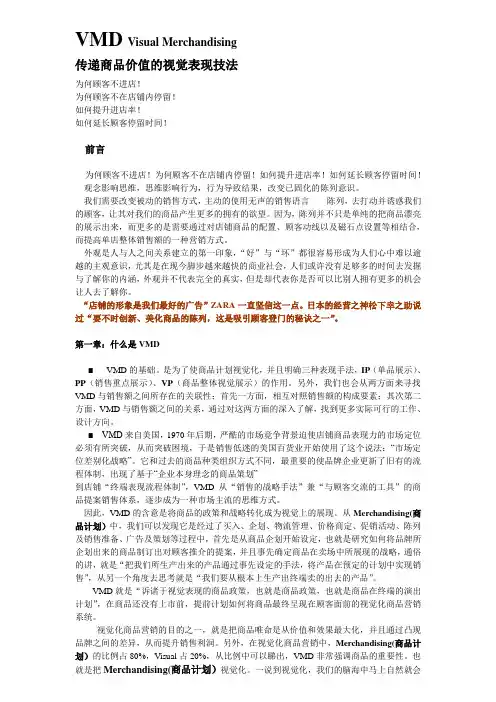
VMD Visual Merchandising传递商品价值的视觉表现技法为何顾客不进店！为何顾客不在店铺内停留！如何提升进店率！如何延长顾客停留时间！前言为何顾客不进店！为何顾客不在店铺内停留！如何提升进店率！如何延长顾客停留时间！观念影响思维，思维影响行为，行为导致结果，改变已固化的陈列意识。

我们需要改变被动的销售方式，主动的使用无声的销售语言------陈列，去打动并诱惑我们的顾客，让其对我们的商品产生更多的拥有的欲望。

因为，陈列并不只是单纯的把商品漂亮的展示出来，而更多的是需要通过对店铺商品的配置、顾客动线以及磁石点设置等相结合，而提高单店整体销售额的一种营销方式。

外观是人与人之间关系建立的第一印象，“好”与“坏”都很容易形成为人们心中难以逾越的主观意识，尤其是在现今脚步越来越快的商业社会，人们或许没有足够多的时间去发掘与了解你的内涵，外观并不代表完全的真实，但是却代表你是否可以比别人拥有更多的机会让人去了解你。

“店铺的形象是我们最好的广告”ZARA一直坚信这一点。

日本的经营之神松下幸之助说过“要不时创新、美化商品的陈列，这是吸引顾客登门的秘诀之一”。

第一章：什么是VMD■ VMD的基础。

是为了使商品计划视觉化，并且明确三种表现手法，IP（单品展示）、PP（销售重点展示）、VP（商品整体视觉展示）的作用。

另外，我们也会从两方面来寻找VMD与销售额之间所存在的关联性；首先一方面，相互对照销售额的构成要素；其次第二方面，VMD与销售额之间的关系，通过对这两方面的深入了解，找到更多实际可行的工作、设计方向。

■ VMD来自美国，1970年后期，严酷的市场竟争背景迫使店铺商品表现力的市场定位必须有所突破，从而突破困境，于是销售低迷的美国百货业开始使用了这个说法：“市场定位差别化战略”。

它和过去的商品种类组织方式不同，最重要的使品牌企业更新了旧有的流程体制，出现了基于“企业本身理念的商品策划”到店铺“终端表现流程体制”，VMD从“销售的战略手法”兼“与顾客交流的工具”的商品提案销售体系，逐步成为一种市场主流的思维方式。

vmd原子配位数
（最新版）
目录
1.VMD 简介
2.原子配位数的定义
3.VMD 中的原子配位数计算方法
4.VMD 原子配位数的应用
5.总结
正文
1.VMD 简介
VMD（Visual Molecular Dynamics）是一款功能强大的分子模拟软件，广泛应用于生物化学、化学和材料科学等领域。

VMD 能够模拟分子体系的各种物理和化学性质，帮助科研人员深入理解分子结构、动力学和热力学特性。

2.原子配位数的定义
原子配位数是指一个原子周围最近的邻近原子数。

在分子中，中心原子与周围原子通过共价键相连，形成一个原子团。

原子配位数反映了原子团中中心原子与周围原子的空间排列和结构特征。

3.VMD 中的原子配位数计算方法
在 VMD 中，原子配位数的计算方法基于分子结构数据。

首先，VMD 通过读取分子结构文件，建立分子模型。

然后，通过算法计算每个原子周围的最近邻原子数。

通常，VMD 使用距离阈值来确定原子间的相互作用。

距离阈值可以根据用户需求进行调整。

4.VMD 原子配位数的应用
VMD 中的原子配位数对于分析分子结构、稳定性和反应性具有重要意义。

科研人员可以通过分析原子配位数来研究分子的结构特征、键长和键角等参数。

此外，原子配位数还可以用于评估分子对接技术的准确性和分子动力学模拟的可靠性。

5.总结
VMD 是一款功能强大的分子模拟软件，能够为科研人员提供丰富的分子结构和性质信息。

在 VMD 中，原子配位数的计算和应用对于研究分子结构和反应性具有重要价值。

VMD之重要性对百货公司而言，VMD之重要性并非今日才受到关注。

在日本从泡沫经济破裂，日本经济进入低成长期，以致变成同业种之间的竞争，他业种之间的竞争，不管到任何店铺去都是相同的商品并列与其店中，差别化可谓比今日还难。

甚于此因，在购买当中则顾客的眼光变的锐利，以诉求方法而言，各家有必要做出自己独特的表现出来。

表现方法而言，虽有各种方法，丹优秀的VMD展现，并非只有形象使之变化而已，最重要的是让顾客有个容易选择、容易购买的百货公司，来支持顾客，这是绝对错不了的。

以百货公司而言，如果把公司招聘拿掉，则看起来每家都一样。

因此要与别家有“差别化”是绝对必要的。

对顾客而言，店铺的特微要比一般无特微的店铺会让顾客容易了解。

总之，“这个商品要买吧”能如此让顾客产生共鸣就好。

对顾客而言在附近最便利的店购买是最好的理由，丹如能缩小商圈的倾向当中，对这家店的忠诚度（对店之信赖性）无法确立，则会产生考虑到别家购买之意识。

以今日这个时期而言，并非把这个商品卖给谁，且这个商品之贩卖方法等之考虑是必要的。

再者有重要的问题，即组织和人才，为什么呢？因为VP工作看起来像多余，因此要VP的营运灵活利用，且要有领导者是绝对需要的，但能得到一般员工飞理解及协助也是必要的。

一、VMD的定义何谓Visual Merchandising(VMD)在了解VMD之前首先应对Merchandising(MD)这个术语要相当的了解才可以。

美国行销协会曾对Merchandising做了下列定义：Merchandising是指将商品或服务，在适当的场所、适当的时机、用适切的数量，以适当的价格提供给消费者的相关计划。

后来又重新定义：Merchandising乃是为了有效实现企业的销售目标，对特定是商品或服务，在一定的场所，一定的时间。

以一定的价格、一定的数量提供给市场的相关计划与管理工作。

因此，MD这个术语，一般而言，是指采购商品，陈列与店铺中贩卖之意。

V M D教程本页仅作为文档封面，使用时可以删除This document is for reference only-rar21year.March简介：这个教程为新用户介绍了VMD的用法。

老用户也可以用本教程进一步熟悉程序的应用，以更好地利用VMD。

本教程是针对VMD 设计的，需要约3个小时来完成。

本教程新增的内容可用三个独立的单元讲解。

第一个单元主要内容是分子图形表现方法基础，还会介绍制作形象逼真的图像要了解的知识。

另外的两个单元是针对高级用户，介绍了VMD的脚本。

尽管非技术性用户可以略去脚本的阅读，但是我们鼓励每个人都去试一试着读一下，因为它会提供一些有力而易用的工具，这些工具是简单的图形用户界面所无法提供的。

本教程以一种有趣的小蛋白质泛素的研究为例来说明VMD的应用。

在本文中，一些资料是在小框中出现的。

这些小框中包括教程的补充内容，例如泛素扮演的生物学角色，使用VMD的一些提示和捷径等等。

如果你有对本教程的评论和问题，请发邮件至。

邮件列表可以在list/tutorial-l/.中找到。

需要的程序：以下是本教程中需要的程序VMD: 可以从下载（在所有平台上均可使用）。

绘图程序：要观看从VMD输出的图像，需要专门的程序。

VMD有一个内置的绘图程序，也可以应用外部程序。

应用什么程序是由你的操作系统决定的。

例如：– Unix/Linux: xmgrace, Windows: Excel, 需要购买)– Mac/Multiple Platforms: Mathematica, 需要购买); gnuplot, 免费下载)现在开始学习VMD你可以在VMD-tutorial-files目录里找到本教程的文件。

如图1所示的VMD-tutorial-files的文件和目录图1：VMD-tutorial-files 的目录结构运行VMD ， 可以在Unix 终端窗口中键入vmd, 在Mac OS X 的应用文件夹中双击VMD 应用程序图标或者在windows 中单击开始——程序——VMD 。

简介：这个教程为新用户介绍了VMD的用法。

老用户也可以用本教程进一步熟悉程序的应用，以更好地利用VMD。

本教程是针对VMD 1.8.3设计的，需要约3个小时来完成。

本教程新增的内容可用三个独立的单元讲解。

第一个单元主要内容是分子图形表现方法基础，还会介绍制作形象逼真的图像要了解的知识。

另外的两个单元是针对高级用户，介绍了VMD的脚本。

尽管非技术性用户可以略去脚本的阅读，但是我们鼓励每个人都去试一试着读一下，因为它会提供一些有力而易用的工具，这些工具是简单的图形用户界面所无法提供的。

本教程以一种有趣的小蛋白质泛素的研究为例来说明VMD的应用。

在本文中，一些资料是在小框中出现的。

这些小框中包括教程的补充内容，例如泛素扮演的生物学角色，使用VMD的一些提示和捷径等等。

如果你有对本教程的评论和问题，请发邮件至******************.edu。

邮件列表可以在/Training/Tutorials/mailing list/tutorial-l/.中找到。

需要的程序：以下是本教程中需要的程序VMD: 可以从/Research/vmd/下载（在所有平台上均可使用）。

绘图程序：要观看从VMD输出的图像，需要专门的程序。

VMD有一个内置的绘图程序，也可以应用外部程序。

应用什么程序是由你的操作系统决定的。

例如：– Unix/Linux: xmgrace, http://plasma-gate.weizmann.ac.il/Grace/– Windows: Excel, /en-us/FX010*********.aspx(需要购买)– Mac/Multiple Platforms: Mathematica, /(需要购买); gnuplot, /(免费下载)现在开始学习VMD你可以在VMD-tutorial-files目录里找到本教程的文件。

如图1所示的VMD-tutorial-files的文件和目录图1：VMD-tutorial-files 的目录结构运行VMD ， 可以在Unix 终端窗口中键入vmd, 在Mac OS X 的应用文件夹中双击VMD 应用程序图标或者在windows 中单击开始——程序——VMD 。

简介：这个教程为新用户介绍了VMD的用法。

老用户也可以用本教程进一步熟悉程序的应用，以更好地利用VMD。

本教程是针对VMD 1.8.3设计的，需要约3个小时来完成。

本教程新增的内容可用三个独立的单元讲解。

第一个单元主要内容是分子图形表现方法基础，还会介绍制作形象逼真的图像要了解的知识。

另外的两个单元是针对高级用户，介绍了VMD的脚本。

尽管非技术性用户可以略去脚本的阅读，但是我们鼓励每个人都去试一试着读一下，因为它会提供一些有力而易用的工具，这些工具是简单的图形用户界面所无法提供的。

本教程以一种有趣的小蛋白质泛素的研究为例来说明VMD的应用。

在本文中，一些资料是在小框中出现的。

这些小框中包括教程的补充内容，例如泛素扮演的生物学角色，使用VMD的一些提示和捷径等等。

如果你有对本教程的评论和问题，请发邮件至******************.edu。

邮件列表可以在/Training/Tutorials/mailing list/tutorial-l/.中找到。

需要的程序：以下是本教程中需要的程序VMD: 可以从/Research/vmd/下载（在所有平台上均可使用）。

绘图程序：要观看从VMD输出的图像，需要专门的程序。

VMD有一个内置的绘图程序，也可以应用外部程序。

应用什么程序是由你的操作系统决定的。

例如：– Unix/Linux: xmgrace, http://plasma-gate.weizmann.ac.il/Grace/– Windows: Excel, /en-us/FX010*********.aspx(需要购买)– Mac/Multiple Platforms: Mathematica, /(需要购买); gnuplot, /(免费下载)现在开始学习VMD你可以在VMD-tutorial-files目录里找到本教程的文件。

如图1所示的VMD-tutorial-files的文件和目录图1：VMD-tutorial-files 的目录结构运行VMD ， 可以在Unix 终端窗口中键入vmd, 在Mac OS X 的应用文件夹中双击VMD 应用程序图标或者在windows 中单击开始——程序——VMD 。

vmd使用手册VMD是生物分子可视化和分析的一种软件工具。

它是一种可视化建模和仿真软件，提供了一套易于使用的工具和功能，用于可视化和分析生物分子的结构和动态。

本文将为您介绍VMD的基本功能、操作步骤和常见用途。

VMD具有多种功能，包括分子可视化、构建和编辑分子、计算和展示分析数据、执行分子动力学模拟等。

它支持多种常见分子文件格式，如PDB、XYZ、MOL2等。

使用VMD，用户可以通过多种方式对分子进行可视化，包括球棍模型、鲍尔模型、Ribbon模型等。

要开始使用VMD，首先需要安装该软件。

可以在VMD官方网站上找到对应的安装包，下载并按照提示进行安装。

安装完成后，启动VMD，在主界面上会出现一个空白视窗。

可以通过"File"菜单中的"New Molecule"选项打开一个分子文件，或者通过拖拽分子文件到VMD窗口中进行导入。

在导入分子文件后，可以通过菜单栏上的各种功能选项进行操作。

例如，"Graphics"菜单中的"Representations"选项可以选择不同的分子表示形式；"Extensions"菜单中的"Extensions"选项提供了一些额外的功能插件，如获取分子表面积、计算氨基酸相互作用等。

VMD还提供了一些常用的快捷键，方便用户进行操作。

例如，按下键盘上的"C"键可以切换分子的表示形式；按下键盘上的"R"键可以旋转分子的视角；按下键盘上的"H"键可以隐藏或显示分子的氢原子等。

除了可视化功能，VMD还提供了一些分子分析和计算功能。

例如，"Extensions"菜单中的"Analysis"选项可以计算分子的RGB颜色、二次结构、排序和聚类等属性；"Extensions"菜单中的"Surfaces"选项可以计算分子的表面积和体积等。

vmd分子动力学模拟均方根位移解释说明以及概述1. 引言1.1 概述本篇文章旨在探讨VMD分子动力学模拟中的均方根位移（root mean square displacement, RMSD）以及其解释说明和应用概述。

VMD（Visual Molecular Dynamics）是一种常用的分子可视化和模拟软件，广泛应用于生物化学、材料科学等领域。

RMSD作为一项重要的计算指标，可以帮助研究人员了解分子系统的运动特征和结构变化情况，对于蛋白质研究以及材料性能预测具有重要意义。

1.2 文章结构本文将按照以下结构展开介绍：引言部分首先从全局上对文章内容进行概述；接着会详细介绍VMD分子动力学模拟和均方根位移的定义与作用，并阐述在VMD中计算均方根位移的方法与原理；随后我们将介绍实验设计与结果分析部分，包括模拟系统的介绍、数据收集与处理方法以及结果分析和讨论；接下来我们会探讨均方根位移在蛋白质研究中的应用以及其对材料性能预测的意义；最后，我们将讨论关于VMD模拟技术发展和改进的前景，并总结本文的主要结论以及可能进行的进一步研究和应用展望。

1.3 目的本文旨在通过对VMD分子动力学模拟均方根位移的解释说明和概述，提供读者对于该领域知识的全面了解。

同时，通过实验设计和结果分析部分，展示均方根位移在蛋白质研究和材料性能预测中的应用意义。

最后，我们也将探讨发展和改进VMD模拟技术的前景，并指出可能进行的进一步研究和应用方向。

通过阅读本文，读者将能够更好地理解VMD分子动力学模拟中均方根位移的概念、计算方法以及其在科学研究中的重要意义。

2. VMD分子动力学模拟均方根位移的解释说明：2.1 VMD分子动力学模拟概述VMD（Visual Molecular Dynamics）是一种用于可视化和分析生物分子系统的软件工具。

它通过从头开始构建分子模型或者导入现有的结构文件，使用经典力学原理进行分子动力学模拟，以模拟和研究分子在特定条件下的运动行为。

The University of Illinois at Urbana-ChampaignNIH Resource for Macromolecular Modeling and Bioinformatics Beckman InstituteComputational Biophysics WorkshopTimeline:a VMD pluginfor trajectory analysisAuthor:Barry IsralewitzJanuary24,2011A current version of this tutorial is available at/Training/Tutorials/CONTENTS2 Contents1Introduction31.1Getting Started (3)1.2Required Programs (4)1.3Timeline in action:examine events in titin domain extension..51.4Per-residue vs.per-selection calculations (7)2Interface and controls10 3Trajectory analysis:titin domain extension153.1Secondary structure during titin domain extension (15)3.2Thresholding and changing appearance:examining RMSF (17)3.3Examine backbone hydrogen bonds during titin extension (18)3.4Using Data Files and Data Collections (19)4Analysis Scripts234.1Simple user-defined all-residue scripts (23)4.2Writing a.tcl script to generate a per-residue.tml datafile (23)4.3Writing a.tcl script to generate a per-selection.tml datafile..271INTRODUCTION3 1IntroductionThis tutorial demonstrates how to use the VMD plugin Timeline to analyze and identify events in molecular dynamics(MD)trajectories.Timeline creates an interactive2D box-plot–time vs.structural component–that can show detailed structural events of an entire system over an entire MD trajectory. Events in the trajectory appear as patterns in the2D plot.The plugin provides several built-in analysis methods,and the means to define new analysis methods. Timeline can read and write data sets,allowing external analysis and plotting with other software packages.Timeline includes features to help analysis of long trajectories and trajectories with large structures.In the main2D box-plot graph,users identify events by looking for patterns of changing values of the analyzed parameter.The user can visually identify regions of interest–rapidly changing structure values,clusters of broken bonds, differences between stable and non-stable values,and similar.The user can explore the resulting structures by tracing the mouse cursor(“scrubbing”)over the identified areas.The structure is highlighted and the trajectory is moved in time to track the highlight.If you have any questions or comments on this tutorial,please email the TCB Tutorial mailing list at tutorial-l@.The mailing list is archived at /Training/Tutorials/mailing list/tutorial-l/.1.1Getting StartedIf you downloaded the tutorial from the web,thefiles that you will be needing can be found in a directory called timeline-tutorial-files.If you received thefiles through a workshop,they can be found in the same directory under the path∼/Workshop/timeline-tutorial.•Unix/Mac OS X Users:In a Terminal window type:cd<path to timeline-tutorial-files directory>You can list the content of this directory,by using the command ls.•Windows Users:Navigate to the timeline-tutorial-files directory using Windows Explorer.This will place you in the directory containing all the necessaryfiles.In the figure below,you can see the structure of this directory.1INTRODUCTION4Figure1:Directory structure for tutorial exercises.Output forfile-writing exercises is provided in the“example output”subdirectory.1.2Required ProgramsThe following programs are required for this tutorial:•VMD:The tutorial assumes that you already have a working knowledge of VMD,which is available at /Research/vmd/ (for all platforms)–The VMD tutorial is available at/Training/Tutorials/vmd/tutorial-html/•a text editor of your choice(we offer a few easy-to-use recommendations):–UNIX:nedit()–Windows XP:WordPad(included with OS).We recommend using WordPad as opposed to NotePad for this tutorial.However,pleaseensure that you save anyfiles in this tutorial as.txt formatfiles,asopposed to.rtf or.docfiles,and to use thefile extensions specifiedin the exercise,e.g..tml.–Mac OS X:Smultron(),TextEdit(included with OS)1INTRODUCTION5a)b)Figure2:Exploring a secondary structure event.Row a)shows the system before the local structure change,row b)shows the system afterwards.The left panels show the entire data plot.The middle panels shows a zoomed-in part of the data plot,and the right panels shows the3D structure of the selected trajectory frame.The vertical bar indicates the current frame.The purple oval, added for thisfigure,shows the rough area of the identified event.See text for additional details.•a command prompt,such as a terminal in UNIX,Terminal.app in Mac OS X, or the DOS command prompt in Windows.Windows users can obtain a command prompt by clicking Start→Programs→Accessories→Com-mand Prompt.1.3Timeline in action:examine events in titin domainextensionThis subsection provides a short run-through of of Timeline features to provide a general idea of how the plugin is ter sections will introduce the display and user interface in greater detail.Here,we look at an MD trajectory of the I91domain of the muscle protein titin.In the simulation trajectory,an external force is applied to the I91domain with the Steered Molecular Dynamics method:one terminus of the domain isfixed and a harmonic restraint moving with constant velocity is applied to the other terminus,causing the domain to extend,unfold,and unravel.The secondary structure changes greatly as the domain unfolds;examining these changes will give us some initial insight into1INTRODUCTION6 how the domain architecture responds to applied force.With the titin I91extension trajectory loaded into VMD,the user starts Timeline by selecting Extension→Analysis→Timeline from the main VMD window,then generates the secondary structure plot by selecting Calculate→Calc.Sec.Structure in the VMD Timeline window.We examine trajectory events which appear as changes in value in the2D plot.As the user moves the highlight cursor around the area of an event in the 2D plot,she can explore the behavior of the3D structure.Figure2illustrates examining an event in a Timeline plot of per-residue secondary structure.By moving the cursor around the event area indicated with a purple oval,the user observes a beta strand,depicted in yellow,losing its secondary structure as it peels away from another beta strand.Note that the purple oval is added for the purposes of this tutorial,the user must normally visually identify the event area. Here the event to notice is the abrupt transition of a horizontal region of yellow to white:part of the domain losing the beta strand character(yellow)it had since the start of the trajectory and becoming random coil(white)as the domain extension proceeds.A user would scrub the mouse highlight cursor around the area of the purple oval,would produce the state shown in Figure2a,before the local structure change,and examine the steps needed to reach Figure2b, after the local structure change has taken place.To“scrub”,click down the left mouse button with the cursor in the area of interest in the2D graph,then move the cursor around the area of interest with the button still depressed–while splitting attention between the2D graph,the changing3D structure,and the changing numerical values displayed in the Highlight Details panel(described below).In Figure3,a plot of salt bridge lifetimes during the titin domain exten-sion trajectory shown in Figure2is displayed,illustrating moving the highlight cursor to examine a salt bridge breaking event.This plot is per-selection;each selection is the pair of residues involved in a salt bridge.Only residue pairs that form a salt bridge for at least one frame of the trajectory are listed.A high-lighted salt bridge is seen breaking between Figure3a and3b.The Timeline highlighted representation can be manipulated like any other VMD representa-tion;here coloring of the highlight was changed from the default ColorID1/red to ResType to show the different residue types of the salt bridge partners,and easily track salt bridge partners as they move apart.In Figure4Timeline’s Threshold Count plot is used to helpfind a suitable color scaling for the plot shown(per-residue Room Mean Square Fluctuation (RMSF)).The Threshold Count is the number of residues or selections in each frame with a value within a given range.As the Threshold Count range controls are adjusted as shown in Figure4b,a pattern with multiple peaks appears (Figure4c),this range is then used to change the color scale,with the result shown in Figure4d.The Threshold Count sliders allow the users to very quickly scan through threshold ranges,without taking the time to redraw the entire2D plot,while still giving an overview of the entire trajectory.1INTRODUCTION7 a)b)Figure3:Exploring a salt bridge breaking event.A Timeline plot of the salt bridges found throughout a trajectory.The structural elements in the vertical axis are selection groups,with each group being the pair of residues involved in a salt bridge.The left panels show the data plot,and the right panels show the3D structure of the selected trajectory frame.The vertical bar indicates the current frame.The purple oval,added to thisfigure,shows the rough area of the identified event.Row a)shows the system before the salt bridge breaks,rowb)shows the system after the salt bridge breaks.See text for additional details.1.4Per-residue vs.per-selection calculationsTimeline plots data about a list of structural elements vs.time.There are two ways of defining the list of structural elements to be analyzed in Timeline.1INTRODUCTION 8a)b)d)c)Figure 4:Using the threshold count to find a color scaling range.The per-residue Root Mean Square Fluctuation (RMSF)plot in a)has color scale set to the default,i.e.,full,data range.Adjusting the Threshold Count range sliders in b)shows multiple peaks in the for the displayed range in c).In d),the 2D plot coloring scale of has been set to the range that was found in c),revealing which structures contribute to the threshold count.Per-residue :a list of residues;the protein and nucleotide residues in the user-defined selection.The default selection is “all”,so this defaults to being a list of all residues in the current molecule.1INTRODUCTION9 Per-selection:a list of any VMD selections.For example,a list of salt bridge pairs,a list of the segments in a large protein complex,a list of of favorite structures in a molecule.These may be defined in built-in functions, listed explicitly,or defined algorithmically in user scripts.2INTERFACE AND CONTROLS 102Interface and controlsThis general description of the Timeline interface should help with navigating in Section 3,“Trajectory Analysis”.Threshold min. / max.Scale/key 2D data plotHighlight details panel Threshold plot (number of residues in each frame within threshold)Current frameCurrent highlight Zoom presetsVertical axis zoomMolecule ID & analysis selectionHorizontal & both-axis zoomVertical axis (structure)Horizontal axis (trajectory frame)Timeline menu bar Threshold count, high, and totalFigure 5:The Timeline 2D data plot.Main interface features are indicated.See a closer view of parts of the interface in Figure 6,and descriptions of these in Table 1.A diagram of the Highlight Details panel is in Figure 7.The top-level Timeline menus are described in Table 2.2INTERFACE AND CONTROLS11a)g)f)e)d)c)b)h)i)k)l)j)Figure 6:Parts of the Timeline interface.a)Horizontal and both-axis zoomsliders,b)Vertical axis zoom slider,c)Threshold count plot,d)Fixed-zoom buttons,e)Highlight Details panel,f)Molecule ID and Analysis selec-tion,g)Key/Scale,h)Key Scale (secondary structure),i)Threshold mini-mum/maximum,j)Threshold count,high,total k)Current structure highlight,l)Current frame highlight2INTERFACE AND CONTROLS 12Analysis method Residue numberResidue name Chain name Segment nameFrame numberUnits ValueFigure 7:Highlight Details panel.2INTERFACE AND CONTROLS13Table1:Timeline main interface featuresInterface element Description See FigureCurrent highlight selec-tion cursor This2D highlight cursor determines the structure that is high-lighted in the3D molecule view,and which is described in the Highlight Details panel.Left mouse button click or drag to change the current highlight selection.5Horizontal axis zoom slider.Scales the2D data plot eful for changing timerange viewed without changing structure range.6aBoth-axis zoom slider.Scales both axes bine with resizing Timelinewindow tofit a larger trajectory or structure in less screen area.6aVertical axis zoom slider.Scales the2D data plot eful for changing range ofstructure data displayed,without changing time range.6b Fixed-zoom buttons.Thefit all button scales the entire loaded trajectory to displaywithin the default window size.The every residue button scalesthe vertical axis to show an axis label for every residue.6dMolecule ID Specifies the molid of the molecule to analyze.6f Analysis selection A VMD selection string,specifies what part of the currentmolecule to use for per-residue analysis.Default is“all”.6fThreshold count plot Graphs number of items(residues or selections)in each framethat are within the threshold range for each frame.The maxvalue is normalized to the height of the graph.First instance ofmax.(min.)value marked with a green(red)line.6cKey/Scale Displays the analysis method,units,and numerical range of cur-rently displayed colors.6g Key/Scale(sec.struct.)When displaying Secondary Structure,displays the structure col-oring codes.The one-letter code descriptions are listed in Help→Structure codes...and in Figure9.6h,92D Data Plot This is a plot of structural elements(residues or selections)vs.time.Exploring this plot for changes,transitions,and visually-detectable correlations helps the userfind events in the trajectory.5Threshold min./max.Set the range for Threshold plot.The Threshold plot will changeas you drag these sliders.The limits of the sliders are adjustedfor the range of the loaded data set.6iThreshold count,high, and total Shows the threshold count for the currently highlighted frame,thehighest threshold count in the trajectory,and the total numberof items in the structure.6jCurrent frame bar The long vertical black bar indicates the current frame,and helpsto visually locate the highlight cursor.5 Current frame highlight Highlight box in the horizontal axis to indicate current frame6l Current structure high-lightHighlight box in the vertical axis to indicate current structure6kMouse zoom-in/zoom-out.Zoom in with right-button click-and-drag;this creates a rectangle selection,the contents of which will expand tofill the2D plot. Zoom out with right click,or with the zoom slider andfixed zoom controls.Scroll Bars Use to move around the2D data block,whenever either scale iszoomed in beyond the“fit all”size.Moves thorugh the structureand the trajectory.5Current structure high-light The long vertical black bar indicates the current frame;this alongwith highlights in the horizontal and vertical axes labels helps visually locate the highlight cursor.5Highlight Details panel Description of the residue/selection beneath the2D cursor.Thecurrent residue number,residue name,chain,segment,and frame,data value for the selected residue,and current analysis method.6e,72INTERFACE AND CONTROLS14Table2:Timeline Top-level MenusTitle DescriptionFile Allows saving and loading formatted data sets,and printing of the 2D data plot.Calculate Provides several built-in calculation options,access to user data fields,and user-defined per-residue functions.Threshold Allows direct entry of values for threshold graph,and clear-ing/recalculating the graph.Analysis Allows a user to enter the user-defined per-residue function,and to set the frame range to which to apply the chosen analysis method. Appearance Sets the value range for scaling on the2D data plot,the shading pallette(greyscale or rainbow),and other user interface details. Data File list of the current data collection,for quick browsing between .tmlfiles in a designated directory.3TRAJECTORY ANALYSIS:TITIN DOMAIN EXTENSION15 3Trajectory analysis:titin domain extensionTo use Timeline to identify events in a trajectory,we must choose which param-eters to examine,perform the required analyses,and explore the resulting2D data sets.We use as an example the titin I91extension trajectory introduced above,and start with examining secondary structure,to get an overall sense of the architectural changes that take place during forced extension.Then we will look at geometricfluctuations during the trajectory,which will both illustrate how to use some of the Timeline tools and provide some hints as to when and where important events are taking place in the I91extension.Then we will look at the hydrogen bond breaking between theβ-strands of the domain’sβ-sheets, to get more insight into how the protein architecture handles applied force. 3.1Secondary structure during titin domain extension We examine how the secondary structure of the domain changes as the force extension takes place.We can see visually by animating the3D trajectory that the domain begins as aβ-sandwich then unravels as the force extension takes place,but there is more to the story;we can make a2D data plot to examine the fate of eachβ-strand.•Start a new VMD unch VMD by:–Unix/Mac OS X Users:typing vmd in a Terminal window.–Windows Users:using the Start menu.•Load in the PSFfile for titin I91domain.In the VMD Main window,select File→New Molecule,then in the Molecule File Browser window,with Load files for:New Molecule selected,navigate to the timeline-tutorial-files directory and select titin.psf.•Load in the titin extension trajectory.In the Molecule File Browser win-dow,with Loadfiles for:0:titin.psf selected,open titin.dcd,which is also in the timeline-tutorial-files directory.The trajectory shows a steered molecular dynamics extension of the I91domain of the giant muscle pro-tein titin,solvated in a water droplet with a non-periodic boundary.•Adjust the VMD Main time slider to frame0.In the VMD Main window, select Graphics→Representations...to display the Graphical Representa-tions window.In the Graphical Representations window,edit the default all selection to not water.Set the Coloring Method to Secondary Struc-ture and Drawing Method to New Cartoon.•Open the Timeline plugin window.In the VMD Main window,select Extension→Analysis→Timeline.•Display secondary structure for all frames,all residues in the trajectory.In the VMD Timeline window,select Calculate→Calc.Sec.Structure3TRAJECTORY ANALYSIS:TITIN DOMAIN EXTENSION16•Scrub the cursor and explore the2D data plot.With left mouse depressed move the2D cursor around the2D data plot.Note how the3D highlight(a red Licorice representation)moves around the molecule,highlightingwhatever is currently under the2D cursor.Figure8:Secondary structure for all residues of I27for all frames of the loaded trajectory.The structure corresponding to the red highlight rectangle in the Timeline(left)data panel is shown in the3D view(right panel).See Figure9 for a magnified view of the color key.•Get detailed information about the trajectory.Details about the residue beneath the2D cursor are shown in the details box to left and below the box plot.The current residue number,residue name,chain,segment,and frame,as well as the data value for the selected residue,and the current analysis method.These change as you move the cursor.•Zoom and scroll around the data plot.Right-mouse-click-and-drag to drawa green-outline box to define the area to zoom into.Right-click will zoomout.The three slider controls on the right side of the Timeline window also control zoom:the vertical slider zooms vertically,the horizontal slider zoom horizontally,the central zoom slider scales the whole data block at once.Thefit all button scales both axes tofit within the standard size of the Timeline window.The every residue button changes the vertical scale to display numbering for every vertical element(residues or selections (covered below,in Section4.3)).•Examine color scale key:The color key for secondary structure attributes is labeled“sec.structure”,and displays the one-letter structure codes used by STRIDE software.The one-letter code descriptions are listed in Help→Structure codes...,and in Figure9.Most relevant here,‘E’(yel-low)corresponds to’Extended conformation’,the main component of beta3TRAJECTORY ANALYSIS:TITIN DOMAIN EXTENSION17T TurnG 3-10 Helix I Pi-helixH Alpha Helix B Isolated Bridge E Extended Con gurationC Coil (none of the above)Figure 9:Color key for secondary structure plots.sheets;‘T’(aqua)corresponds to “Turn”,another beta sheet component,and ‘C’(white)stands for “Coil”(random coil,no structure).Note that secondary structure is a special case for coloring;for all other cases of calculations,the color scale shows a numerical range.•Identify the time frames when each of the individual β-strands begins to lose secondary structure,and when it has completely lost secondary structure.3.2Thresholding and changing appearance:examiningRMSFThere are two related ways to help examine how the values of a data set are distributed:first,by using the Threshold Count tool;second,by changing the color scaling range of the 2D plot.The Threshold Count tool adds up,for each frame,the number of residues or selections that fall within a given range,then plots these numbers for all frames.The plot is dynamically updated as the Threshold Min and Max values are changed.Here we review how to do this for the Root Mean Square Fluctuation data set examined in Figure 4,then use the results from this to set the color scaling range,in order to identify which structures are involved in the fluctuation events.•Display root mean square fluctuation for all frames,all residues in the trajectory.In the VMD Timeline window,select Calculate →Calc.RMSF •Use the thresholding tools.Adjust the Threshold Plot by changing the Threshold Min and Threshold Max bounds sliders.(Type in values here with select Threshold →Set bounds...Set them to 4.48and 6.67and note the repeating pattern of peaks.This thresholding can change much more3TRAJECTORY ANALYSIS:TITIN DOMAIN EXTENSION18 quickly than we can adjust the2D plot(especially for a large plot)and can track changes hard to total up by eye.The Threshold plot updates as the range is changed,to allow quick exploration of the plots.Now apply the threshold bounds values we set to the coloring of the whole2D plot: select Appearance→Set scaling...and enter4.48and6.67as bottom and top values.The result should resemble Figure4c.Scrub the highlight cursor over the transitions in the resultant plot to see what structures are involved in thefluctuation increases.More on changing appearance.Perform other changes to the Timeline plot,to see features that may be helpful when working with different data sets or different structures:•Toggle display of one letter vs.three letter residue codes in the vertical plot labels by selecting Appearance→Show1-letter codes.•With the Analysis Selection set to all,or to any interesting sub-selection, make an RMSF plot as before with Calculate→Calc.RMSF.Change the2D Plot color scale with Appearance→Color scale→Rainbow and Appearance→Color scale→Grayscale.•For more experimentation with this specific trajectory,source a TCL script to load the example system in the state shown in Figures2and3,with car-toon representation and coloring showing native secondary structure.To this,start a new VMD session,change directory using the VMD Tk termi-nal to timeline-tutorial-files,then enter into the VMD Tk terminal source start-titin.vmd.Note that thisfile sources titin-struct.vmd in the same directory.The latter Tcl script imposes the known native secondary structure of the published structure,in order to show more ac-curate beta-strands at trajectory start compared to that determined from the built-in secondary structure algorithm(STRIDE).3.3Examine backbone hydrogen bonds during titin ex-tensionNow we will look at the hydrogen bond breaking pattern during the I91extension trajectory.Since we are looking at the protein architecture,we will examine the bonds between the partnerβ-strands that make up the twoβ-sheets which form the I91domainβ-sandwich.•Change the Analysis Selection from all to name N HN O C,to select only the atoms involved in inter-β-stand hydrogen bonds.•Calculate the hydrogen bonds that can be formed with the current se-lection,in Calculate→Calc.H-bonds....Enter a Bond distance cutoffof3.5and an Angle cutoff(deg)of45,then click the Calculate button.Theresult should resemble Figure10.3TRAJECTORY ANALYSIS:TITIN DOMAIN EXTENSION19•The value of data in the2D plot is either0or1.Set the Threshold Plotrange from0to1to see the number of formed hydrogen bonds in eachframe.(Although the auto-ranging is already set from0to1,you muststill adjust the threshold minimum control once to display the ThresholdPlot).•Zoom in the plot to examine individual hydrogen bonds.Click on theatoms in the3D view to display the names and numbers of the residuesinvolved.•Use the hydrogen bond plot,and thefit all button,to look for overallpatterns of hydrogen bonds breaking.Look for H-bond breaking—theend of a white horizontal line—clustered around the same time,and checkthe associated structures.While using a copy of a secondary structure plotsuch as Figure8for reference,note whichβ-strands the bond breakingsare associated with,and how they relate to the beginning/ending times ofsecondary structure loss(unraveling)of individualβ-strands.•Load in a version of the I91extension trajectory with four times as manyframes(four times the temporal detail):naviage to to the examples directory and load titin-big.dcd•We will examine a set of inter-β-strand hydrogen bonds that are stableduring equilibration of I91.Change directory to the examples directoryand typesource stable-titin-backbone-hbonds.tcl in the Tk console.Thiswill add two vmd atom macros:backboneHSel and backboneOSel.•Change the analysis selection to backboneHSel or backboneOSel.•Select Calculate→Calc.H-bonds...and click the Calculate button.•Scrub through the trajectory with the highlight cursor,using the Thresh-old count tool to note how the hydrogen bond count has the largest dropbetween frames11and18.Note where these breaking H-bonds are in the2D view,as in the previous example.•Add both CPK and Hbond graphic representations as for selection backboneHSel or backboneOSel.Note the hydrogen bonds ending in the2D graph be-tween frames11and18,and how they correspond to the hydrogen break-ing in the3D view,as shown in Figure11.These simultaneous hydrogenbond breaking seen in Figure11c is what is responsible for the extensionforce peak seen in Figure11a.Under forced extension,I91architecturecannot allow further unraveling until these bonds are broken.3.4Using Data Files and Data CollectionsThese features help with saving and loading completed calculations(so you won’t have to spend time calculating them again),and with creating and brows-ing sets of pre-computed calculations.3TRAJECTORY ANALYSIS:TITIN DOMAIN EXTENSION20•Export and Import the calculated data.Select File→Write Data File...and save as test-rmsf.tml.Clear the plot with Calculate→Clear data, then read the datafile back in with File→Load Data File...,and specify the test-rmsf.tml you just saved.•Use a data collection:With the titin trajectory loaded,select Data→Set Data Collection directory...and select titin-data-coll in the dialog box, which is in the timeline-tutorial-files directory.•The Data menu is now populated with the.tmlfiles in that directory, select each to load that calculation data.Select Data→titin-strand-contacts.tml,then Data→titin-h-bonds.tml,etc.Loading each data set will reset the coloring range of the2D plot to the full range of each loaded set.•Try making a new directory,save two or more.tmlfiles to it,then display the contents via the Data menu.。

变分模态分解过程讲解1.引言在实际应用中，许多信号都是由多个不同频率的成分叠加而成的。

传统的时频分析方法往往无法对这种信号进行准确的分解和分析。

而VMD是一种灵活、高效的信号分解方法，能够将多模态信号分解为一组单模态成分，并恢复出每个成分对应的频率、幅值和相位信息。

2.基本原理VMD的基本原理是将信号分解为一组成分和一个残差项，成分项由信号中的单一模态成分组成，而残差项包含信号中未被成分分解的部分。

每个成分都是由正交模态函数（OMF，Orthogonal Mode Functions）构成，这些函数是一组正交、指数型的函数。

3.VMD的分解过程VMD的分解过程可以分为以下四个步骤：步骤1:数据预处理首先，对原始信号进行预处理，去除可能存在的基线漂移和高频噪声，以减小干扰。

步骤2:模态函数初始化初始化正交模态函数（OMF）。

OMF的数量等于预设的成分数量。

初始化时可以使用高斯函数、指数函数或者正弦函数。

步骤3:模态分解在这一步中，将信号分解为一组模态函数和一个残差项。

为了最小化信号与模态函数之间的离散KL散度（Kullback-Leibler Divergence），通过交替优化模态函数和权值的方式进行迭代。

首先，在固定权值的条件下，通过使用Hilbert-Huang变换得到信号的频率信息，并根据频率信息更新OMF的相位。

然后，在固定OMF相位的条件下，通过使用降序排序的方式得到OMF 的频率信息，更新每个OMF的辅助变量，并根据辅助变量的信息更新OMF 的赋权。

以上两个步骤交替进行，直到满足停止准则（如误差小于一些阈值，或者迭代次数达到设定值）。

步骤4:重构原始信号将分解得到的模态函数相加，得到原始信号的近似重构。

同时，将残差项加到重构信号中，恢复原始信号。

4.算法特点VMD具有以下几个特点：a.VMD是一种自适应的分解方法，不需要预先设定信号模态数目。

b.VMD能够恢复每个成分的频率、幅值和相位信息。

引言：在前文中，我们已经介绍了VMD软件的基本概念和使用方法。

本文将继续探讨VMD软件的着色方法，重点介绍不同的着色方法及其应用。

着色方法是用来将分子结构中的原子或分子团体以不同的颜色呈现出来，以便于更好地理解和分析分子结构。

通过深入学习和理解这些着色方法，我们可以更加准确地解读和解释分子模拟结果，并有助于科学家们从中获得更多有价值的信息。

概述：本文将围绕VMD软件的着色方法展开讨论，总结了各种不同的着色方法及其应用领域。

这些方法包括球棍式着色法、域着色法、电荷着色法、高级实验数据显色法和自定义着色法。

正文内容：1. 球棍式着色法1.1 介绍：球棍式着色法是最常见的着色方法之一，它将原子和键以球和棍的形式表示。

球代表原子，棍代表键。

1.2 应用：球棍式着色法可以用来显示分子的整体结构，帮助我们观察分子的几何形状和连接方式。

1.3 优点：简单直观，易于理解和分析。

1.4 缺点：对于大分子或复杂结构的分子来说，球棍式着色法可能会过于拥挤，难以观察细节。

2. 域着色法2.1 介绍：域着色法通过将原子或分子团体按照其性质或功能分配不同的颜色来表示。

2.2 应用：域着色法广泛应用于蛋白质结构的表示和分析中，可以用来显示氨基酸的类型、二级结构和功能区域等。

2.3 优点：能够更清晰地显示分子的功能区域和结构特征。

2.4 缺点：可能会忽略原子间的细节信息。

3. 电荷着色法3.1 介绍：电荷着色法通过根据原子的电荷分布将其着色，以显示电荷在分子中的分布情况。

3.2 应用：电荷着色法主要用于研究分子的电子性质和反应机制，可以帮助我们理解分子的电子云分布和电荷转移过程。

3.3 优点：能够直观地显示电荷的分布情况。

3.4 缺点：不适用于没有电荷信息的分子。

4. 高级实验数据显色法4.1 介绍：高级实验数据显色法是利用一系列实验数据（如核磁共振谱和X射线衍射数据）来给分子着色，以反映实验结果。

4.2 应用：高级实验数据显色法可以帮助我们解析实验数据，以揭示分子的结构和性质。