Supersymmetric left-right model and scalar potential

a r X i v :h e p -p h /9404257v 1 12 A p r 1994DESY 94-061ISSN 0418-9833April 1994hep-ph/9404257Can the Supersymmetric µparameter be generated dynamically without a light Singlet?Ralf Hempfling Deutsches Elektronen-Synchrotron,Notkestraße 85,D-22603Hamburg,Germany ABSTRACTIt is generally assumed that the dynamical generation of the Higgs mass param-eter of the superpotential,µ,implies the existence of a light singlet at or below the supersymmetry breaking scale,M SUSY .We present a counter-example in which the singlet field can receive an arbitrarily heavy mass (e.g.,of the order of the Planck scale,M P ≈1019GeV).In this example,a non-zero value of µis generatedthrough soft supersymmetry breaking parameters and is thus naturally of the order of M SUSY .The cancellation of quadratic divergences in the unrenormalized Green func-tions is one of the main motivations of supersymmetry(SUSY).It stabilizes any mass scale under radiative corrections and thus allows the existence of different mass scales such as the electroweak scale,given by the Z boson mass,m z,and the Planck scale,M P.The minimal supersymmetric standard model(MSSM)is the most popular model of this kind due to its minimal particle content[1].In this model,the SU(2)L⊗U(1)Y symmetry breaking is driven by soft SUSY break-ing parameters.Thus,the SUSY breaking scale,M SUSY,has to be at or slightly above m z.For this mechanism to work it is also necessary that the SUSY Higgs mass parameter,|µ|<∼M SUSY.This parameter also determines the chargino and neutralino mass spectrum.From here one can deduce a experimental lower bound from LEP experiments of|µ|>∼m z/4independent of tanβ[2].The fact that in the MSSM theµ-parameter,which is a priori arbitrary,has to lie within the narrow range1will be evaded[5].We will demonstrate in the following that it is also possible to make N1heavy [say m N1=O(M P)]while keeping N1 =O(M SUSY)withoutfine-tuning.In this limit we recover the predictive Higgs sector of the MSSM[6]with its well defined upper limit of the lightest Higgs boson mass[eq.(2)].First we need to extend the symmetry group of our Lagrangian in order to forbid the explicit Higgs mass term of the superpotential,W H=µH8(ξ+2N∗1N1−2N∗2N2−N∗3N3)2.(4)Here the inclusion of a Fayet-Iliopoulos term[7],ξ,is the easiest way of breaking the U(1)Y′gauge symmetry but one can envisage other alternatives[8].The VEVs are denoted byn1= N1 =0,n2= N2 =1λ+ λ2+4ξ , n3= N3 = λ.(5)The CP-even and CP-odd components of the scalarfield N1are mass-degenerate mass-eigenstates with m N1=(m2+λ2n23)1/2.The gauge boson,g′,acquires a massm g′=g′(n22+n23/4)1/2via the Higgs mechanism.The masses of the remaining CP-,m g′(m N1,0;the zero mass eigenvalue corresponds even(CP-odd)scalars are m N1to the Goldstone boson which is absorbed to give mass to the gauge boson).Theand±m g′as required if mass eigenvalues of the fermionic components are±m N1SUSY is unbroken.Note that in addition to the gauge and the SUSY transformations the La-grangian is invariant under the global U(1)R-symmetry[9]which does not com-mute with SUSY.This symmetry transformsΦ→exp(inΦα)Φ,where nΦ= 2,0,0,0for the bosons and n Φ=1,−1,−1,1for the fermions(Φ=N1,N2,N3,g′). We now break SUSY explicitly in the standard fashion by including soft SUSY breaking terms[10]V soft=BmN1N2−AλN1N23+h.c.,(6) where A,B=O(M SUSY)are the soft SUSY breaking parameters.With these terms the R-symmetry is broken down to a discrete Z2symmetry(α=±π).If we minimize the full potential,V=V SUSY+V soft,wefindN1 ≈(A−B)mn2ξ.However,the condition N1 =0is protected by R-symmetry to all orders in perturbation theory and is only broken by adding soft SUSY breaking terms[eq.(6)].We now include in our model the full particle content of the MSSM.The Z2symmetry is equivalent to the usual R-parity that prevents baryon and lepton number violating interactions. The full superpotential can then be written asW=W N+W H+W Y,(8) where W H=κN1Hof W in eq.(8)and by requiring the absence of anomalies.These constraints can be satisfied by introducing additional pairs of SUSY multiplets T∼(n c,n w,Y,Y′1) and T c∼(¯n c,n w,−Y,Y′2).These representations have been included in pairs such√that below the U(1)Y′breaking scale,Useful conversations with W.Buchm¨u ller are gratefully ac-knowledgedREFERENCES1.H.P.Nilles,Phys.Rep.110,1(1984);H.E.Haber and G.L.Kane,Phys.Rep.117,75(1985);R.Barbieri,Riv.Nuovo Cimento11,1(1988).2.J.-F.Grivaz,in Proceedings of the Workshop on e+e−Collisions at500GeV:The Physics Potential,Munich,Annecy,Hamburg,DESY report DESY92-123B(1992).3.G.F.Guidice and A.Masiero,Phys.Lett.B206,480(1988);J.E.Kimand H.P.Nilles,Phys.Lett.B263,79(1991);J.A.Casas and C.Mu˜n oz, Phys.Lett.B306,288(1993).4.E.Witten,Phys.Lett.B105,267(1981);L.Ib´a˜n ez and G.G.Ross,Phys.Lett.B110,215(1982);P.V.Nanopoulos and K.Tamvakis,Phys.Lett.B113,151(1982).5.see,e.g.,J.Ellis,J.F.Gunion,H.E.Haber,L.Roszkowski and F.Zwirner,Phys.Rev.D39,844(1989).6.see,e.g.,J.F.Gunion,H.E.Haber,G.L.Kane,and S.Dawson,The HiggsHunter’s Guide,(Addison-Wesley,Redwood City,CA,1990).7.P.Fayet and J.Iliopoulos,Phys.Lett.B51,461(1974).8.e.g.,L.O’Raifeartaigh,Nucl.Phys.B96,331(1975).9.P.Fayet,Nucl.Phys.B90,104(1975);A.Salam and J.Strathdee,Nucl.Phys.B87,85(1975).10.L.Girardello and M.T.Grisaru,Nucl.Phys.B194,65(1982).。

a r X i v :0803.2889v 2 [h e p -p h ] 14 J u l 2008Mapping Out SU (5)GUTs with Non-Abelian Discrete Flavor SymmetriesFlorian Plentinger ∗and Gerhart Seidl †Institut f¨u r Physik und Astrophysik,Universit¨a t W¨u rzburg,Am Hubland,D 97074W¨u rzburg,Germany(Dated:December 25,2013)We construct a class of supersymmetric SU (5)GUT models that produce nearly tribimaximal lepton mixing,the observed quark mixing matrix,and the quark and lepton masses,from discrete non-Abelian flavor symmetries.The SU (5)GUTs are formulated on five-dimensional throats in the flat limit and the neutrino masses become small due to the type-I seesaw mechanism.The discrete non-Abelian flavor symmetries are given by semi-direct products of cyclic groups that are broken at the infrared branes at the tip of the throats.As a result,we obtain SU (5)GUTs that provide a combined description of non-Abelian flavor symmetries and quark-lepton complementarity.PACS numbers:12.15.Ff,11.30.Hv,12.10.Dm,One possibility to explore the physics of grand unified theories (GUTs)[1,2]at low energies is to analyze the neutrino sector.This is due to the explanation of small neutrino masses via the seesaw mechanism [3,4],which is naturally incorporated in GUTs.In fact,from the perspective of quark-lepton unification,it is interesting to study in GUTs the drastic differences between the masses and mixings of quarks and leptons as revealed by current neutrino oscillation data.In recent years,there have been many attempts to re-produce a tribimaximal mixing form [5]for the leptonic Pontecorvo-Maki-Nakagawa-Sakata (PMNS)[6]mixing matrix U PMNS using non-Abelian discrete flavor symme-tries such as the tetrahedral [7]and double (or binary)tetrahedral [8]groupA 4≃Z 3⋉(Z 2×Z 2)and T ′≃Z 2⋉Q,(1)where Q is the quaternion group of order eight,or [9]∆(27)≃Z 3⋉(Z 3×Z 3),(2)which is a subgroup of SU (3)(for reviews see, e.g.,Ref.[10]).Existing models,however,have generally dif-ficulties to predict also the observed fermion mass hierar-chies as well as the Cabibbo-Kobayashi-Maskawa (CKM)quark mixing matrix V CKM [11],which applies especially to GUTs (for very recent examples,see Ref.[12]).An-other approach,on the other hand,is offered by the idea of quark-lepton complementarity (QLC),where the so-lar neutrino angle is a combination of maximal mixing and the Cabibbo angle θC [13].Subsequently,this has,in an interpretation of QLC [14,15],led to a machine-aided survey of several thousand lepton flavor models for nearly tribimaximal lepton mixing [16].Here,we investigate the embedding of the models found in Ref.[16]into five-dimensional (5D)supersym-metric (SUSY)SU (5)GUTs.The hierarchical pattern of quark and lepton masses,V CKM ,and nearly tribi-maximal lepton mixing,arise from the local breaking of non-Abelian discrete flavor symmetries in the extra-dimensional geometry.This has the advantage that theFIG.1:SUSY SU (5)GUT on two 5D intervals or throats.The zero modes of the matter fields 10i ,5H,24H ,and the gauge supermul-tiplet,propagate freely in the two throats.scalar sector of these models is extremely simple without the need for a vacuum alignment mechanism,while of-fering an intuitive geometrical interpretation of the non-Abelian flavor symmetries.As a consequence,we obtain,for the first time,a realization of non-Abelian flavor sym-metries and QLC in SU (5)GUTs.We will describe our models by considering a specific minimal realization as an example.The main features of this example model,however,should be viewed as generic and representative for a large class of possible realiza-tions.Our model is given by a SUSY SU (5)GUT in 5D flat space,which is defined on two 5D intervals that have been glued together at a common endpoint.The geom-etry and the location of the 5D hypermultiplets in the model is depicted in FIG.1.The two intervals consti-tute a simple example for a two-throat setup in the flat limit (see,e.g.,Refs.[17,18]),where the two 5D inter-vals,or throats,have the lengths πR 1and πR 2,and the coordinates y 1∈[0,πR 1]and y 2∈[0,πR 2].The point at y 1=y 2=0is called ultraviolet (UV)brane,whereas the two endpoints at y 1=πR 1and y 2=πR 2will be referred to as infrared (IR)branes.The throats are supposed to be GUT-scale sized,i.e.1/R 1,2 M GUT ≃1016GeV,and the SU (5)gauge supermultiplet and the Higgs hy-permultiplets 5H and2neously broken to G SM by a 24H bulk Higgs hypermulti-plet propagating in the two throats that acquires a vac-uum expectation value pointing in the hypercharge direc-tion 24H ∝diag(−12,13,15i ,where i =1,2,3is the generation index.Toobtainsmall neutrino masses via the type-I seesaw mechanism [3],we introduce three right-handed SU (5)singlet neutrino superfields 1i .The 5D Lagrangian for the Yukawa couplings of the zero mode fermions then readsL 5D =d 2θ δ(y 1−πR 1) ˜Y uij,R 110i 10j 5H +˜Y d ij,R 110i 5H +˜Y νij,R 15j5i 1j 5H +M R ˜Y R ij,R 21i 1j+h.c. ,(3)where ˜Y x ij,R 1and ˜Y x ij,R 2(x =u,d,ν,R )are Yukawa cou-pling matrices (with mass dimension −1/2)and M R ≃1014GeV is the B −L breaking scale.In the four-dimensional (4D)low energy effective theory,L 5D gives rise to the 4D Yukawa couplingsL 4D =d 2θ Y u ij 10i 10j 5H +Y dij10i 5H +Y νij5i ∼(q i 1,q i 2,...,q i m ),(5)1i ∼(r i 1,r i 2,...,r im ),where the j th entry in each row vector denotes the Z n jcharge of the representation.In the 5D theory,we sup-pose that the group G A is spontaneously broken by singly charged flavon fields located at the IR branes.The Yukawa coupling matrices of quarks and leptons are then generated by the Froggatt-Nielsen mechanism [21].Applying a straightforward generalization of the flavor group space scan in Ref.[16]to the SU (5)×G A represen-tations in Eq.(5),we find a large number of about 4×102flavor models that produce the hierarchies of quark and lepton masses and yield the CKM and PMNS mixing angles in perfect agreement with current data.A distri-bution of these models as a function of the group G A for increasing group order is shown in FIG.2.The selection criteria for the flavor models are as follows:First,all models have to be consistent with the quark and charged3 lepton mass ratiosm u:m c:m t=ǫ6:ǫ4:1,m d:m s:m b=ǫ4:ǫ2:1,(6)m e:mµ:mτ=ǫ4:ǫ2:1,and a normal hierarchical neutrino mass spectrumm1:m2:m3=ǫ2:ǫ:1,(7)whereǫ≃θC≃0.2is of the order of the Cabibbo angle.Second,each model has to reproduce the CKM anglesV us∼ǫ,V cb∼ǫ2,V ub∼ǫ3,(8)as well as nearly tribimaximal lepton mixing at3σCLwith an extremely small reactor angle 1◦.In perform-ing the group space scan,we have restricted ourselves togroups G A with orders roughly up to 102and FIG.2shows only groups admitting more than three valid mod-els.In FIG.2,we can observe the general trend thatwith increasing group order the number of valid modelsper group generally increases too.This rough observa-tion,however,is modified by a large“periodic”fluctu-ation of the number of models,which possibly singlesout certain groups G A as particularly interesting.Thehighly populated groups would deserve further system-atic investigation,which is,however,beyond the scopeof this paper.From this large set of models,let us choose the groupG A=Z3×Z8×Z9and,in the notation of Eq.(5),thecharge assignment101∼(1,1,6),102∼(0,3,1),103∼(0,0,0),52∼(0,7,0),52↔4FIG.3:Effect of the non-Abelian flavor symmetry on θ23for a 10%variation of all Yukawa couplings.Shown is θ23as a function of ǫfor the flavor group G A (left)and G A ⋉G B (right).The right plot illustrates the exact prediction of the zeroth order term π/4in the expansion θ23=π/4+ǫ/√2and the relation θ13≃ǫ2.The important point is that in the expression for θ23,the leading order term π/4is exactly predicted by thenon-Abelian flavor symmetry G F =G A ⋉G B (see FIG.3),while θ13≃θ2C is extremely small due to a suppression by the square of the Cabibbo angle.We thus predict a devi-ation ∼ǫ/√2,which is the well-known QLC relation for the solar angle.There have been attempts in the literature to reproduce QLC in quark-lepton unified models [26],however,the model presented here is the first realization of QLC in an SU (5)GUT.Although our analysis has been carried out for the CP conserving case,a simple numerical study shows that CP violating phases (cf.Ref.[27])relevant for neutri-noless double beta decay and leptogenesis can be easily included as well.Concerning proton decay,note that since SU (5)is bro-ken by a bulk Higgs field,the broken gauge boson masses are ≃M GUT .Therefore,all fermion zero modes can be localized at the IR branes of the throats without intro-ducing rapid proton decay through d =6operators.To achieve doublet-triplet splitting and suppress d =5pro-ton decay,we may then,e.g.,resort to suitable extensions of the Higgs sector [28].Moreover,although the flavor symmetry G F is global,quantum gravity effects might require G F to be gauged [29].Anomalies can then be canceled by Chern-Simons terms in the 5D bulk.We emphasize that the above discussion is focussed on a specific minimal example realization of the model.Many SU (5)GUTs with non-Abelian flavor symmetries,however,can be constructed along the same lines by varying the flavor charge assignment,choosing different groups G F ,or by modifying the throat geometry.A de-tailed analysis of these models and variations thereof will be presented in a future publication [30].To summarize,we have discussed the construction of 5D SUSY SU (5)GUTs that yield nearly tribimaximal lepton mixing,as well as the observed CKM mixing matrix,together with the hierarchy of quark and lepton masses.Small neutrino masses are generated only by the type-I seesaw mechanism.The fermion masses and mixings arise from the local breaking of non-Abelian flavor symmetries at the IR branes of a flat multi-throat geometry.For an example realization,we have shown that the non-Abelian flavor symmetries can exactly predict the leading order term π/4in the sum rule for the atmospheric mixing angle,while strongly suppress-ing the reactor angle.This makes this class of models testable in future neutrino oscillation experiments.In addition,we arrive,for the first time,at a combined description of QLC and non-Abelian flavor symmetries in SU (5)GUTs.One main advantage of our setup with throats is that the necessary symmetry breaking can be realized with a very simple Higgs sector and that it can be applied to and generalized for a large class of unified models.We would like to thank T.Ohl for useful comments.The research of F.P.is supported by Research Train-ing Group 1147“Theoretical Astrophysics and Particle Physics ”of Deutsche Forschungsgemeinschaft.G.S.is supported by the Federal Ministry of Education and Re-search (BMBF)under contract number 05HT6WWA.∗********************************.de †**************************.de[1]H.Georgi and S.L.Glashow,Phys.Rev.Lett.32,438(1974);H.Georgi,in Proceedings of Coral Gables 1975,Theories and Experiments in High Energy Physics ,New York,1975.[2]J.C.Pati and A.Salam,Phys.Rev.D 10,275(1974)[Erratum-ibid.D 11,703(1975)].[3]P.Minkowski,Phys.Lett.B 67,421(1977);T.Yanagida,in Proceedings of the Workshop on the Unified Theory and Baryon Number in the Universe ,KEK,Tsukuba,1979;M.Gell-Mann,P.Ramond and R.Slansky,in Pro-ceedings of the Workshop on Supergravity ,Stony Brook,5New York,1979;S.L.Glashow,in Proceedings of the 1979Cargese Summer Institute on Quarks and Leptons, New York,1980.[4]M.Magg and C.Wetterich,Phys.Lett.B94,61(1980);R.N.Mohapatra and G.Senjanovi´c,Phys.Rev.Lett.44, 912(1980);Phys.Rev.D23,165(1981);J.Schechter and J.W. F.Valle,Phys.Rev.D22,2227(1980);zarides,Q.Shafiand C.Wetterich,Nucl.Phys.B181,287(1981).[5]P.F.Harrison,D.H.Perkins and W.G.Scott,Phys.Lett.B458,79(1999);P.F.Harrison,D.H.Perkins and W.G.Scott,Phys.Lett.B530,167(2002).[6]B.Pontecorvo,Sov.Phys.JETP6,429(1957);Z.Maki,M.Nakagawa and S.Sakata,Prog.Theor.Phys.28,870 (1962).[7]E.Ma and G.Rajasekaran,Phys.Rev.D64,113012(2001);K.S.Babu,E.Ma and J.W.F.Valle,Phys.Lett.B552,207(2003);M.Hirsch et al.,Phys.Rev.D 69,093006(2004).[8]P.H.Frampton and T.W.Kephart,Int.J.Mod.Phys.A10,4689(1995); A.Aranda, C. D.Carone and R.F.Lebed,Phys.Rev.D62,016009(2000);P.D.Carr and P.H.Frampton,arXiv:hep-ph/0701034;A.Aranda, Phys.Rev.D76,111301(2007).[9]I.de Medeiros Varzielas,S.F.King and G.G.Ross,Phys.Lett.B648,201(2007);C.Luhn,S.Nasri and P.Ramond,J.Math.Phys.48,073501(2007);Phys.Lett.B652,27(2007).[10]E.Ma,arXiv:0705.0327[hep-ph];G.Altarelli,arXiv:0705.0860[hep-ph].[11]N.Cabibbo,Phys.Rev.Lett.10,531(1963);M.Kobayashi and T.Maskawa,Prog.Theor.Phys.49, 652(1973).[12]M.-C.Chen and K.T.Mahanthappa,Phys.Lett.B652,34(2007);W.Grimus and H.Kuhbock,Phys.Rev.D77, 055008(2008);F.Bazzocchi et al.,arXiv:0802.1693[hep-ph];G.Altarelli,F.Feruglio and C.Hagedorn,J.High Energy Phys.0803,052(2008).[13]A.Y.Smirnov,arXiv:hep-ph/0402264;M.Raidal,Phys.Rev.Lett.93,161801(2004);H.Minakata andA.Y.Smirnov,Phys.Rev.D70,073009(2004).[14]F.Plentinger,G.Seidl and W.Winter,Nucl.Phys.B791,60(2008).[15]F.Plentinger,G.Seidl and W.Winter,Phys.Rev.D76,113003(2007).[16]F.Plentinger,G.Seidl and W.Winter,J.High EnergyPhys.0804,077(2008).[17]G.Cacciapaglia,C.Csaki,C.Grojean and J.Terning,Phys.Rev.D74,045019(2006).[18]K.Agashe,A.Falkowski,I.Low and G.Servant,J.HighEnergy Phys.0804,027(2008);C.D.Carone,J.Erlich and M.Sher,arXiv:0802.3702[hep-ph].[19]Y.Kawamura,Prog.Theor.Phys.105,999(2001);G.Altarelli and F.Feruglio,Phys.Lett.B511,257(2001);A.B.Kobakhidze,Phys.Lett.B514,131(2001);A.Hebecker and J.March-Russell,Nucl.Phys.B613,3(2001);L.J.Hall and Y.Nomura,Phys.Rev.D66, 075004(2002).[20]D.E.Kaplan and T.M.P.Tait,J.High Energy Phys.0111,051(2001).[21]C.D.Froggatt and H.B.Nielsen,Nucl.Phys.B147,277(1979).[22]Y.Nomura,Phys.Rev.D65,085036(2002).[23]H.Georgi and C.Jarlskog,Phys.Lett.B86,297(1979).[24]H.Arason et al.,Phys.Rev.Lett.67,2933(1991);H.Arason et al.,Phys.Rev.D47,232(1993).[25]D.S.Ayres et al.[NOνA Collaboration],arXiv:hep-ex/0503053;Y.Hayato et al.,Letter of Intent.[26]S.Antusch,S.F.King and R.N.Mohapatra,Phys.Lett.B618,150(2005).[27]W.Winter,Phys.Lett.B659,275(2008).[28]K.S.Babu and S.M.Barr,Phys.Rev.D48,5354(1993);K.Kurosawa,N.Maru and T.Yanagida,Phys.Lett.B 512,203(2001).[29]L.M.Krauss and F.Wilczek,Phys.Rev.Lett.62,1221(1989).[30]F.Plentinger and G.Seidl,in preparation.。

a r X i v :0805.4481v 1 [h e p -t h ] 29 M a y 2008SUPERSYMMETRIC CHERN-SIMONS MODELS IN HARMONIC SU-PERSPACESB.M.ZupnikBogoliubov Laboratory of Theoretical Physics,JINR,Dubna,Moscow Region,141980,Russia;E-mail:zupnik@theor.jinr.ruAbstractWe review harmonic superspaces of the D =3,N =3and 4supersymmetries and gauge models in these superspaces.Superspaces of the D =3,N =5supersymmetry use harmonic coordinates of the SO (5)group.The superfield N =5actions describe the off-shell infinite-dimensional Chern-Simons supermultiplet.1IntroductionSupersymmetric extensions of the D =3Chern-Simons theory were discussed in [1]-[10].A superfield action of the D =3,N =1Chern-Simons theory can be interpreted as the superspace integral of the differential Chern-Simons superform dA +2iwhere i andˆk are two-component indices of the automorphism groups SU L(2)and SU R(2), respectively,αis the two-component index of the SL(2,R)group and m=0,1,2is the 3D vector index.The N=4supersymmetry transformations areδx m=−i(γm)αβ(ǫαjˆk θβjˆk−iǫβjˆkθαjˆk),(2.2)whereγm are the3Dγmatrices.The SU L(2)/U(1)harmonics u±i[11]can be used to construct the left analytic super-space[15]with the LA coordinatesζL=(x m L,θ+ˆkα).(2.3)The L-analytic prepotential V++(ζL,u)describes the left N=4vector multiplet A m,φˆkˆl ,λαiˆk,D ik.The D=3,N=4SY M action can be constructed in terms of this prepotential by anal-ogy with the D=4,N=2SY M action[14].Let us introduce the new notation for the left harmonics u±i=u(±1,0)iand the analogousnotation v(0,±1)ˆk for the right SL R(2)/U(1)harmonics.The biharmonic N=4superspaceuses the Grassmann coordinates[15]θ(±1,±1)α=u(±1,0)i v(0,±1)ˆkθiˆkα.(2.4)In this representation,we haveζL=(x m L,θ(1,±1)α),V++≡V(2,0),(2.5)D(1,±1)αV(2,0)=0,D(0,2)vV(2,0)=0.(2.6)The right analytic N=4coordinates areζR=(x m R,θ(±1,1)α),x m R=x m L−2i(γm)αβθ(−1,1)αθ(1,1)β.(2.7) The mirror R analytic prepotentialˆV(0,2)D(±1,1)ˆV(0,2)=0,D(2,0)uˆV(0,2)=0(2.8)describes the right N=4vector multipletˆA m,ˆφij,ˆλαiˆk ,ˆD ik,whereˆA m is the mirror vectorgaugefield using the independent gauge group.The right N=4SY M action is similar to the analogous left action.These multiplets can be formally connected by the map SU L(2)↔SU R(2).The N=4superfield Chern-Simons type(or BF-type)action for the gauge group U(1)×U(1)connects two mirror vector multipletsdud3x L dθ(−4,0)V(2,0)(ζL,u)D(1,1)αD(1,1)αˆV(0,−2),(2.9) where the right connection satisfies the equationD(0,2)v ˆV(0,−2)=D(0,−2)v˜V(0,2),D(2,0)uˆV(0,−2)=0.(2.10)The component form of this action was considered in[16,17].We can identify the left and right isospinor indices in the N=4spinor coordinatesθαjˆk→θαjk=θα(jk)+12D++αD++αV−−.(2.14)The action of the corresponding CS-theory can be constructed in the full or analytic N=3superspaces[8,9].3Harmonic superspaces for the group SO(5)The homogeneous space SO(5)/U(2)is parametrized by elements of the harmonic5×5 matrixU K a=(U+i a,U0a,U−ia)=(U+1a,U+2a,U0a,U−1a,U−2a),(3.1) where a=1,...5is the vector index of the group SO(5),i=1,2is the spinor index of the group SU(2),and U(1)-charges are denoted by symbols+,−,0.The basic relations for these harmonics areU+i a U+k a=U+i a U0a=0,U−ia U−ka =U−ia U0a=0,U+i a U−ka=δi k,U0a U0a=1,U+i a U−ib +U−ia U+ib+U0a U0b=δab.(3.2)We consider the SO(5)invariant harmonic derivatives with nonzero U(1)charges∂+i=U+i a ∂∂U−ia,∂+i U0a=U+i a,∂+i U−ka=−δi k U0a,∂++=U+ia∂∂U0a −U0a∂∂U+i a ,[∂−i,∂−k]=εki∂−−,∂−k∂−k=−∂−−,where some relations between these harmonic derivatives are defined.The U(1)neutral harmonic derivatives form the Lie algebra U(2)∂i k=U+i a ∂∂U−ia,[∂+i,∂−k]=−∂i k,(3.4)∂0≡∂k k=U+k a ∂∂U−ka,[∂++,∂−−]=∂0,∂i k U+l a=δl k U+i a,∂i k U−la =−δi l U−ka.(3.5)The operators∂+k,∂++,∂−k ,∂−−and∂i k satisfy the commutation relations of the Lie al-gebra SO(5).One defines an ordinary complex conjugation on these harmonicsU0a=U0a,(3.6) however,it is convenient to use a special conjugation in the harmonic space(U+i a)∼=U+i a,(U−ia)∼=U−ia,(U0a)∼=U0a.(3.7) All harmonics are real with respect to this conjugation.The full superspace of the D=3,N=5supersymmetry has the spinor CB coordi-natesθαa,(α=1,2;a=1,2,3,4,5)in addition to the coordinates x m of the three-dimensional Minkowski space.The group SL(2,R)×SO(5)acts on the spinor coordinates. The superconformal transformations of these coordinates are considered in Appendix.The SO(5)/U(2)harmonics allow us to construct projections of the spinor coordinates and the partial spinor derivativesθ+iα=U+i aθαa,θ0α=U0aθαa,θ−αi=U−iaθαa,(3.8)∂−iα=∂/∂θ+iα,∂0α=∂/∂θ0α,∂+iα=∂/∂θ−αi.The analytic coordinates(AB-representation)in the full harmonic superspace use these projections of10spinor coordinatesθ+iα,θ0α,θ−αi and the following representation of the vector coordinate:x m A ≡y m=x m+i(θ+kγmθ−k)=x m+i(θaγmθb)U+k a U−kb.(3.9)The analytic coordinates are real with respect to the special conjugation. The harmonic derivatives have the following form in AB:D+k=∂+k−i(θ+kγmθ0)∂m+θ+kα∂0α−θ0α∂+kα,D++=∂+++i(θ+kγmθ+k )∂m+θ+αk∂+kα,(3.10)D k l=∂k l+θ+kα∂−lα−θ−αl∂−kα.We use the commutation relations[D+k,D+l]=−εkl D++,D+k D+k=D++.(3.11) The AB spinor derivatives areD+iα=∂+iα,D−iα=−∂−iα−2iθ−βi∂αβ,D0α=∂0α+iθ0β∂αβ.(3.12) The coordinates of the analytic superspaceζ=(y m,θ+iα,θ0α,U K a)have the Grass-mann dimension6and dimension of the even space3+6.The functionsΦ(ζ)satisfy the Grassmann analyticity condition in this superspaceD+kαΦ=0.(3.13)In addition to this condition,the analytic superfields in the SO (5)/U (2)harmonic super-space possess also the U (2)-covariance.This subsidiary condition looks especially simple for the U (2)-scalar superfieldsD k l Λ(ζ)=0.(3.14)The integration measure in the analytic superspace dµ(−4)has dimension zerodµ(−4)=dUd 3x A (∂0α)2(∂−iα)4=dUd 3x A dθ(−4).(3.15)The SO (5)/U (1)×U (1)harmonics can be defined via the components of the real orthogonal 5×5matrix [20,21]U Ka = U (1,1)a ,U (1,−1)a ,U (0,0)a ,U (−1,1)a ,U (−1,−1)a (3.16)where a is the SO(5)vector index and the index K =1,2,...5corresponds to givencombinations of the U(1)×U(1)charges.We use the following harmonic derivatives∂(2,0)=U (1,1)b∂/∂U (−1,1)b−U (1,−1)b∂/∂U (−1,−1)b,∂(1,1)=U (1,1)b∂/∂U (0,0)b −U (0,0)b∂/∂U (−1,−1)b,∂(1,−1)=U (1,−1)b ∂/∂U (0,0)b−U (0,0)b∂/∂U (−1,1)b,∂(0,2)=U (1,1)b∂/∂U (1,−1)b−U (−1,1)b∂/∂U (−1,−1)b,∂(0,−2)=U (1,−1)b∂/∂U (1,1)b−U (−1,−1)b∂/∂U (−1,1)b.(3.17)We define the harmonic projections of the N =5Grassmann coordinatesθK α=θaαU K a =(θ(1,1)α,θ(1,−1)α,θ(0,0)α,θ(−1,1)α,θ(−1,−1)α).(3.18)The SO (5)/U (1)×U (1)analytic superspace contains only spinor coordinatesζ=(x m A ,θ(1,1)α,θ(1,−1)α,θ(0,0)α),(3.19)x m A=x m +iθ(1,1)γm θ(−1,−1)+iθ(1,−1)γm θ(−1,1),δǫx m A =−iǫ(0,0)γm θ(0,0)−2iǫ(−1,1)γm θ(1,−1)−2iǫ(−1,−1)γm θ(1,1),(3.20)where ǫKα=ǫαa U Ka are the harmonic projections of the supersymmetry parameters.General superfields in the analytic coordinates depend also on additional spinor coor-dinates θ(−1,1)αand θ(−1,−1)α.The harmonized partial spinor derivatives are∂(−1,−1)α=∂/∂θ(1,1)α,∂(−1,1)α=∂/∂θ(1,−1)α,∂(0,0)α=∂/∂θ(0,0)α,(3.21)∂(1,1)α=∂/∂θ(−1,−1)α,∂(1,−1)α=∂/∂θ(−1,1)α.We use the special conjugation ∼in the harmonic superspaceU (p,q )a =U (p,−q )a ,θ(p,q )α=θ(p,−q )α, x m A =x m A,(θ(p,q )αθ(s,r )β)∼=θ(s,−r )βθ(p,−q )α, f (x A )=¯f(x A ),(3.22)where ¯fis the ordinary complex conjugation.The analytic superspace is real with respect to the special conjugation.The analytic-superspace integral measure contains partial spinor derivatives(3.21)1dµ(−4,0)=−they are traceless and anti-HermitianΛ†=−Λ.We treat these prepotentials as connections in the covariant gauge derivatives∇+i=D+i+V+i,∇++=D+++V++,δΛV+i=D+iΛ+[Λ,V+i],δΛV++=D++Λ+[Λ,V++],(4.4) D+kαδΛV+k=D+kαδΛV++=0,D i jδΛV+k=δk jδΛV+i,D i jδΛV++=δi jδΛV++,where the infinitesimal gauge transformations of the gauge superfields are defined.These covariant derivatives commute with the spinor derivatives D+kαand preserve the CR-structure in the harmonic superspace.We can construct three analytic superfield strengths offthe mass shellF++=112πdµ(−4)Tr{V+j D++V+j+2V++D+j V+j+(V++)2+V++[V+j,V+j]},(4.5)where k is the coupling constant,and a choice of the numerical multiplier guarantees the correct normalization of the vector-field action.This action is invariant with respect to the infinitesimal gauge transformations of the prepotentials(4.4).The idea of construction of the superfield action in the harmonic SO(5)/U(2)was proposed in[18],although the detailed construction of the superfield Chern-Simons theory was not discussed in this work.The equivalent superfield action was considered in the framework of the alternative superfield formalism[20].The superconformal N=5invariance of this action was proven in[19].The action S1yields superfield equations of motion which mean triviality of the su-perfield strengths of the theoryF(+3) k =D++V+k−D+kV+++[V++,V+k]=0,F++=V++−D+k V+k −V+k V+k=0.(4.6)These classical superfield equations have pure gauge solutions for the prepotentials onlyV+k=e−ΛD+k eΛ,V++=e−ΛD++eΛ,(4.7) whereΛis an arbitrary analytic superfield.The transformation of the sixth supersymmetry can be defined on the analytic N=5 superfieldsδ6V++=ǫα6D0αV++,δ6V+k=ǫα6D0αV+k,(4.8)δ6D+k V+l=ǫα6D0αD+k V+l,δ6D++V+l=ǫα6D0αD++V+l,(4.9) whereǫα6are the corresponding odd parameters.This transformation preserves the Grass-mann analyticity and U(2)-covariance{D0α,D+kβ}=0,[D k l,D0α]=0,[D+k,D0α]=D+kα,[D++,D0α]=0.(4.10)The action S1is invariant with respect to this sixth supersymmetryδ6S1= dµ(−4)ǫα6D0αL(+4)=0.(4.11)In the SO(5)/U(1)×U(1)harmonic superspace,we can introduce the D=3,N=5 analytic matrix gauge prepotentials corresponding to thefive harmonic derivativesV(p,q)(ζ,U)=[V(1,1),V(1,−1),V(2,0),V(0,±2)],(V(1,1))†=−V(1,−1),(V(2,0))†=V(2,0),V(0,−2)=[V(0,2)]†,(4.12) where the Hermitian conjugation†includes∼conjugation of matrix elements and trans-position.We shall consider the restricted gauge supergroup using the supersymmetry-preserving harmonic(H)analyticity constraints on the gauge superfield parametersH1:D(0,±2)Λ=0.(4.13) These constrains yield additional reality conditions for the component gauge parameters.We use the harmonic-analyticity constraints on the gauge prepotentialsH2:V(0,±2)=0,D(0,−2)V(1,1)=V(1,−1),D(0,2)V(1,1)=0(4.14) and the conjugated constraints combined with relations(4.12).The superfield CS action can be constructed in terms of these H-constrained gauge superfields[21]2ikS=−V(2,0)V(2,0)}.(4.15)2Note,that the similar harmonic superspace based on the USp(4)/U(1)×U(1)harmon-ics was used in[22]for the harmonic interpretation of the D=4,N=4super Yang-Mills constraints.This work was partially supported by the grants RFBR06-02-16684,DFG436RUS 113/669-3,INTAS05-10000008-7928and by the Heisenberg-Landau programme.References[1]W.Siegel,Nucl.Phys.B156(1979)135.[2]J.Schonfeld,Nucl.Phys.B185(1981)157.[3]B.M.Zupnik,D.G.Pak,Teor.Mat.Fiz.77(1988)97;Eng.transl.:Theor.Math.Phys.77(1988)1070.[4]B.M.Zupnik,D.G.Pak,Class.Quant.Grav.6(1989)723.[5]B.M.Zupnik,Teor.Mat.Fiz.89(1991)253,Eng.transl.:Theor.Math.Phys.89(1991)1191.[6]B.M.Zupnik,Phys.Lett.B254(1991)127.[7]H.Nishino,S.J.Gates,Int.J.Mod.Phys.8(1993)3371.[8]B.M.Zupnik,D.V.Khetselius,Yad.Fiz.47(1988)1147;Eng.transl.:Sov.J.Nucl.Phys.47(1988)730.[9]B.M.Zupnik,Springer Lect.Notes in Phys.524(1998)116;hep-th/9804167.[10]J.H.Schwarz,Jour.High.Ener.Phys.0411(2004)078,hep-th/0411077.[11]A.Galperin,E.Ivanov,S.Kalitzin,V.Ogievetsky,E.Sokatchev,Class.Quant.Grav.1(1984)469.[12]A.Galperin,E.Ivanov,S.Kalitzin,V.Ogievetsky,E.Sokatchev,Class.Quant.Grav.2(1985)155.[13]A.Galperin,E.Ivanov,V.Ogievetsky,E.Sokatchev,Harmonic superspace,Cam-bridge University Press,Cambridge,2001.[14]B.M.Zupnik,Phys.Lett.B183(1987)175.[15]B.M.Zupnik,Nucl.Phys.B554(1999)365,Erratum:Nucl.Phys.B644(2002)405E;hep-th/9902038.[16]R.Brooks,S.J.Gates,Nucl.Phys.B432(1994)205,hep-th/09407147.[17]A.Kapustin,M.Strassler,JHEP04(1999)021,hep-th/9902033.[18]P.S.Howe,M.I.Leeming,Clas.Quant.Grav.11(1994)2843,hep-th/9402038.[19]B.M.Zupnik,Chern-Simons theory in SO(5)/U(2)harmonic superspace,arXiv0802.0801(hep-th).[20]B.M.Zupnik,Phys.Lett.B660(2008)254,arXiv0711.4680(hep-th).[21]B.M.Zupnik,Gauge model in D=3,N=5harmonic superspace,arXiv0708.3951(hep-th).[22]I.L.Buchbinder,O.Lechtenfeld,I.B.Samsonov,N=4superparticle and super Yang-Mills theory in USp(4)harmonic superspace,arxiv:0804.3063(hep-th).。

逻辑斯蒂增长英语
逻辑斯蒂增长（Logistic Growth）的英文是：Logistic Growth。

逻辑斯蒂增长模型，又称自我限制增长模型，是一种描述种群增长速率先增加后减小，呈“S”型曲线的数学模型。

它是生物学、生态学和数学等学科中常用的一种模型。

这种模型在生态学和流行病学等领域中尤为重要，因为它能够描述资源有限的情况下种群或疾病的增长情况。

在逻辑斯蒂增长模型中，种群的增长率与种群大小成反比，当种群大小接近环境容纳量时，增长率逐渐减小，最终趋于零。

这个模型可以用微分方程来描述，也可以通过离散时间递推公式来模拟。

analysis is best.The chapter then moves into detailed, step-by-step instructions on how to run each analysis. The coverage of these procedures is,necessarily,a bit more detailed than the other sections because most users will not be familiar with the specific features of each test.Finally,Chapter15includes four different out-standing laboratory exercises that use JWatcher to teach students:(1)how to develop their own ethogram and score behavior,(2)the differences between time sampling and continuous recordings, (3)how to conduct sequential analysis,and(4)how to use both sequential analysis and basic analysis to refine research questions from initial pilot data.These exercises use video clips downloadable from the JWatcher website free of charge and would be excellent teaching tools in the classroom.This manual is a vast improvement over the Version0.9Manual available on the JWatcher website, which only covers some basic guidelines for running the software,explains what the individual file types do,and indicates how to analyze results.The online manual has no coverage of the complex sequential analysis functions of JWatcher1.0.In summary,this book is a necessity for users at all experience levels who wish to quantify behavior using an event recorder.JWatcher software is free of charge and this manual is affordable enough that several copies could be purchased for use in one’s research laboratory.The money from the sale of the manual is used to support further development of the software so that the future versions of the program can be offered free of charge.Theodore StankowichOrganismic&Evolutionary BiologyUniversity of Massachusetts Amherst Morrill Science Center South,611N.Pleasant Street,Amherst,MA01003E-mail:Advance Access publication February14,2008doi:10.1093/icb/icn005An Introduction to Nervous Systems. Ralph J.Greenspan,editor.Woodbury,NY:Cold Spring Harbor Laboratory Press,2007. 172pp.ISBN978-0-87969-0(hardcover)$65.00,ISBN 978-0-87969-821-8(paper)$45.00.Over the past30years,there have been several iterations of books aimed at capturing in brief the essence of the organization and function of the nervous system.Not uncommonly,they extract general princi-ples that would be more fully explored in a compre-hensive text but do not otherwise deviate significantly from the traditional form and content of presentation. This one does.Ralph Greenspan is an established neuroscientist who has pioneered novel research to explore basic and cognitive aspects of nervous system function using the fruit fly as a model system.As he states in the Preface of this book,the Neurocience Institute,of which he is a staff scientist,aims to be a provocative academy,to“push the envelope.”That philosophy is clearly conveyed in the creative,non-traditional style of presentation in this special book. The title of the book,“An Introduction to Nervous Systems,”is a bit misleading.A more accurate title, although cumbersome,would be something like “An Introduction to Nervous Systems through Exam-ination of Some Invertebrate Models.”The book uses select examples from invertebrate nervous systems to convey some fundamental principles that apply in some respects to the organization and function of thenervous system in general.In the final,short chapter—“Are All Brains Alike?Are All Brains Different?”—theauthor writes“Perhaps all nervous systems make useof common general strategies.Anatomical disparitiesmay mask underlying functional similarities in thetasks performed by various circuits.”At first glance,it is surprising that nowhere in thetext are there descriptions of what has been learnedabout ion channels and membrane potentials from classical studies of squid giant axons;of neuralnetwork properties from studies of the crustacean stomatogastric ganglion;of nervous system develop-ment from experiments on fruit fly nerve cord or nematode worms;of sensory signaling and receptionfrom the moth or cricket;or of insect social structure,for example.The author’s enthusiasm for Drosophila,which represents his main research subject,is reflectedin a substantial fraction of the book.Moreover,thereis little or no discussion of how the principles described are employed in mammals.Surveying thebreadth of the neurobiology landscape seems not to bethe primary purpose of this book.Rather,it describesselect examples that highlight what studies of“simple”invertebrate nervous systems have taught us.The taleslink organization of the nervous system to the organism’s behavior,for which invertebrates haveproven to be especially valuable.In a modern, molecular,mammalian research universe,the rich439 Downloaded from https:///icb/article/48/3/439/627027 by Guangxi University of Nationalities user on 18 September 2023history of fundamental contributions of invertebrates to neuroscience may too often be overlooked.It is especially in this respect that the book is a welcome contribution to the neurobiological literature.In the introduction to Chapter4—“Modulation,The Spice of Neural Life”—the author writes:“The capabilities of invertebrates have traditionally been underesti-mated.Perhaps this is because they are not warm and fuzzy...For whatever reason,it has taken us an inordinately long time to realize that even the simplest animals have the capacity for modifying their behavior by adjusting the activities of their nervous systems. Perhaps this is a fundamental,inseparable property of nervous systems.”Despite the fact that the book deviates from a traditional style,in its own way it follows a rather traditional sequence,e.g.,membrane potentials,then chemical signaling and sensing,then neural circuits,then neuromodulation,then biological clocks,then higher,or cognitive,function.There is a lot to like in this book,not only in its fascinating content but in the style of presentation. Ralph Greenspan weaves a tapestry about the molecular,cellular and network origins of function and behavior,and the implications for speciation, using a variety of invertebrate models.The images he creates are expressed as interesting,often humorous, readable stories about what some nervous systems do, how they do it,and how that has evolved using some basic principles in novel ways.Each chapter begins with a relevant quote or poem from a literary or scientific giant that sets the stage and tone for the often poetic introduction and description that follows. The stories themselves—about swimming in Paramecium and jellyfish,light detection by barnacles, decision making by marine snails,circadian rhythms, flying,and mating—are fascinating because they are set in a context of understanding the generation and modulation of behavior and,in some cases,the impact on ecology and evolution.Although the author states in the Preface that the book is intended for the neurobiology novice posses-sing a basic introductory knowledge of biology,this reviewer believes that it would be more appropriate for an individual with an introductory neurobiological background.For example,in the very first chapter, one quickly discovers that understanding“simple”systems can be quite complex.In particular,students new to neurobiology often struggle with concepts underlying the generation of membrane potentials and the relationship of voltage and current,yet the text and figures require some understanding of these topics.In this respect,the Glossary at the end of the book seems uneven,defining some very basic biological terms yet not defining“receptor potential,”for example,which is named but not explained in the caption of Figure3.10.Not to quibble,but this reviewer and two other neuroscientists who scanned the book question some statements or generalizations proposed,particularly in the Introduction(“What are Brains For”?).For example,on page1it states“When it comes to brains,size unquestionably matters.”While that is no doubt true,it may be the organization of cells,i.e.the way they interact,that is more relevant.If it is size that is so important,then one should note that about three quarters of cells in mammalian brain are glial cells, not neurons,some potentially capable of modulating chemical signaling at up to100,000synapses,yet their contributions are not mentioned(see below). Furthermore,spinal cords also possess much of the organization and cellular interactions,e.g.,integrating sensory input and generating motor output,yet we view their capabilities as somewhat lacking in comparison with brain.What might be the funda-mental differences between invertebrate and verte-brate nervous systems and between brain and spinal cord that yield unique aspects of functional compe-tence?Or,are they as different as we imagine them to be,particularly in comparing function in invertebrates versus vertebrates?These are some interesting questions—not found in a typical comprehensive text—that might be explored a bit further in the Introduction and perhaps elsewhere in the book.In addition,on page2,the author writes“Chemical sensing is almost certainly the original sense...,”yet mechanically gated ion channels that could sense changes in flow or pressure in the ambient environ-ment are universal and also have been identified in prokaryotic organisms.Also,on page4,the author writes“And because none of us wants to submit to being experimented upon...we study animals.”Yet, there is a substantial and rapidly growing literature that provides insights on the organization and function of human brain from studies of living persons—for example from functional MRI or stimulation/recording of brain of awake epileptic patients—or of postmortem tissue samples.There are several other aspects of the book in its current form that would benefit from revision in a second edition.First,the emphasis is on how invertebrate nervous systems inform on nervous systems in general,but it is not clear in many cases to what extent the general organization of the behaviors is similar in invertebrates and vertebrates or whether similar molecules or mechanisms are used for different purposes.Does evolution mix and match bits and pieces of behavioral components that moves behavior in new directions?One also wonders whether440Book ReviewsDownloaded from https:///icb/article/48/3/439/627027 by Guangxi University of Nationalities user on 18 September 2023there are good examples of invertebrate nervous systems and behaviors that do not translate well to a mammalian equivalent.Second,the book has a traditional neurocentric focus—and some inverte-brates indeed have few glial cells—yet in the past couple of decades it has become abundantly clear from studies of mammalian systems that interactions of neurons with glia play vital roles in regulation of neural function,development and blood flow.Third, some of the figures could benefit from greater clarity or correction of the illustration or of the explanation in the caption,including citing the source link that is listed in the Bibliography at the end of the book.In addition,the Preface could note the location of the relevant Bibliography,currently organized by chapters but separate from them.It should be noted that the author also recently co-edited a much more compre-hensive(800pages),related book(“Invertebrate Neurobiology”)with Geoffrey North.In summary,this is an excellent book for gaining an appreciation for the links between form-function and behavior in the nervous system from invertebrate model systems and one that is interesting and enjoyable to read.It should be particularly valuable in inspiring budding or established life scientists to read more on the subject or even to become engaged in the pursuit of elucidating fundamental principles of neurobiology and behavior.It should stimulate broad questions about nervous systems and behavior. From a pedagogical perspective,I could imagine it being assigned as a short text in a general course on neurobiology and behavior or in a specialized neurobiology course that focuses on invertebrates or as a supplement to a more comprehensive text.Robert M.GrossfeldDepartment of Zoology NC State University,Raleigh,NC27695E-mail:*************************Advance Access publication February15,2008doi:10.1093/icb/icn004Rodent Societies–An Ecological and Evolutionary Perspective.Jerry O.Wolff and Paul W.Sherman,editors. Chicago,IL:University of Chicago Press,2007.610pp. ISBN0-226-90536-5(cloth),$125.00and ISBN0-226-90537-3(paper),$49.00.As the editors point out in the first sentence of the first chapter,“The Rodentia is the largest order of mammals consisting of more than2000species and comprising44%of all mammals.”This breadth makes the task of compiling a definitive and comprehensive anthology on rodent societies a nearly impossible task,but the result is undoubtedly the most exhaustive and progressive analysis of rodent social behavior to date.Deftly edited by Jerry Wolff and Paul Sherman,this well-organized book,consisting of41chapters from61contributors is,without doubt,a significant compendium of more than50years of research.That being said,only a true rodent lover is likely to love this book.Its creation was prompted by the success of the two volumes within this series that preceded it:Primate Societies and Cetacean Societies(published by University of Chicago Press).Thus,the scope and format of Rodent Societies is in many ways similar to that of the previous two volumes.The text is organized into nine sections,beginning with a succinct,but satisfying,overview of rodent evolutionary history and proceeding through sexual behavior,life histories and behavior,behavioral development,social behavior, antipredator behavior,comparative socioecology,con-servation and disease,and a final concluding sectionwritten by the editors on potential directions for future research.Each chapter concludes with a summary thatbriefly reviews the material,identifies caveats,and frequently suggests strategies for future research.The chapters are written by some of the most productiveand well-known scholars in the field but,as expected ina multi-authored work,the quality is uneven.Some chapters do a better job than others of achieving thestated goal to“synthesize and integrate the currentstate of knowledge about the social behavior of rodents”and to“provide ecological and evolutionary contexts for understanding rodent societies.”However,it generally succeeds in combining ideasand strategies from a wide range of disciplines to generate new theoretical and experimental paradigmsfor exploring rodent social behavior.Despite this,itfeels outdated in many places.Much of the work citedin the text is not new,with the majority of citationsdating before2000and a substantial number datingbefore1985.Even the photographs,all in black andwhite,are fairly old and some date back to the1950s.Some of the illustrations are even hand-drawn.Thismakes the book feel like historical retrospective rathera breakthrough collaborative of evolutionary and behavioral biology.441 Downloaded from https:///icb/article/48/3/439/627027 by Guangxi University of Nationalities user on 18 September 2023。

理了一些曾经读过而且觉得很不错的理论物理参考书，希望能对想做或者正在做理论物理的人有点用。

１:经典力学/电动力学/统计力学/量子力学1.1: Greiner系列,其实不止四大力学，覆盖面从Mechanics到QCD,基本都不错，物理图像非常清晰明了。

还有Schwabl写的两本书 Quantum Mechanics&Advanced Quantum Mechanics，应该比传统的经典教材容易念一些。

1.2: 传统的经典教材，Landau系列,Goldstein的经典力学,Jackson的电动力学， Schiff，Sakurai的量子力学，不用多说了。

2:量子场论/标准模型2.1: 前面提到的Greiner系列，Mandl&Shaw的Quantum Field Theory,Ryder的Quantum Field Theory，Brown的Quantum Field Theory以及Bailin&Love的Introduction to Gauge Field Theory,比较容易念。

2.2: Peskin&schroeder，绝对经典。

2.3: Cheng&Li的Gauge Theory of Elementary Particle Physics，也是经典。

2.4: Itzykson&Zuber的Quantum Field Theory,Pokorski的Gauge Field Theories, 可能难一些，但是是非常好的参考书。

2.5: Muta的Foundations of Quantum Chromodynamics，通俗易懂。

2.6: Martin的讲义Phenomenology of Particle Physics，值得一看。

2.7: Boehm,Denner&Joos的Gauge Theories of the Strong and Electroweak Interaction, 做Particle Phenomenology的话绝对案头必备书目。

斯佩里左右脑分工理论 对斯佩里左右脑分工理论的认识 美国心理生物学家斯佩里博士（Roger Wolcott Sperry，1913.8.20—1994.4.17）通过著名的割裂脑实验，证实了大脑不对称性的“左右脑分工理论”，因此荣获1981年度的“诺贝尔生理学或医学奖”。

正常人的大脑有两个半球，大脑两半球之间由胼胝体连接沟通，构成一个完整的统一体。

在正常的情况下，大脑是作为一个整体来工作的，来自外界的信息，经胼胝体传递，左、右两个半球的信息可在瞬间进行交流（以每秒10亿位元的速度彼此交流），人的每一种活动都是两半球信息交换和综合的结果。

大脑两半球在机能上有分工，左半球感受并控制右边的身体，右半球感受并控制左边的身体。

所谓割裂脑实验就是将大脑左、右两个半球之间的胼胝体割断，外界信息传至大脑半球皮层的某一部分后，不能同时又将此信息通过横向胼胝体纤维传至对侧皮层相对应的部分，每个半球各自独立地进行活动，彼此不能知道对侧半球的活动情况。

从1952年至 1961年的10年里，斯佩里先用猫、猴子、猩猩做了大量的割裂脑实验，取得了一些成绩，为以后做“裂脑人”的研究奠定了基础。

从1961年开始，斯佩里把“裂脑人”作为研究大脑两半球各种机能的研究对象，对“裂脑人”长时间进行了一系列的实验研究。

由割裂脑实验得知：左半脑主要负责逻辑理解、记忆、时间、语言、判断、排列、分类、逻辑、分析、书写、推理、抑制、五感(视、听、嗅、触、味觉)等，思维方式具有连续性、延续性和分析性。

因此左脑可以称作“意识脑”、“学术脑”、“语言脑”。

右半脑主要负责空间形象记忆、直觉、情感、身体协调、视知觉、美术、音乐节奏、想像、灵感、顿悟等，思维方式具有无序性、跳跃性、直觉性等。

斯佩里认为右脑具有图像化机能，如企划力、创造力、想像力；与宇宙共振共鸣机能，如第六感、透视力、直觉力、灵感、梦境等；超高速自动演算机能，如心算、数学；超高速大量记忆，如速读、记忆力。

Munkres算法，也称为匈牙利算法，是一种用于解决二分图最大匹配问题的线性时间复杂度算法。

二分图最大匹配问题是在一个二分图中寻找最大的匹配，即找到最大的子集，使得图中的每条边都有一个与之匹配的顶点。

Munkres算法的基本思想是通过在原图中构造增广路径，并在增广路径上不断进行增广操作，最终得到最大匹配。

具体步骤如下：
1. 初始化：将所有未匹配的点标记为0，已匹配的点标记为无穷大。

2. 寻找增广路径：从任意一个未匹配的点开始，进行DFS或BFS 等搜索方法，直到找到一个增广路径。

增广路径是指从起点开始，沿着一条路径可以一直匹配到终点，但终点尚未匹配。

3. 进行增广操作：在增广路径上，将路径上的所有点与对应的未匹配点进行匹配，并将这些点标记为已匹配。

4. 重复步骤2和3，直到所有的点都已匹配或者找不到增广路径为止。

Munkres算法的时间复杂度为O(V^3)，其中V是顶点的数量。

这是因为在最坏的情况下，需要枚举所有可能的增广路径，而每条增广路径最多包含V个顶点。

因此，Munkres算法是一种非常高效的算法，被广泛应用于解决二分图最大匹配问题。

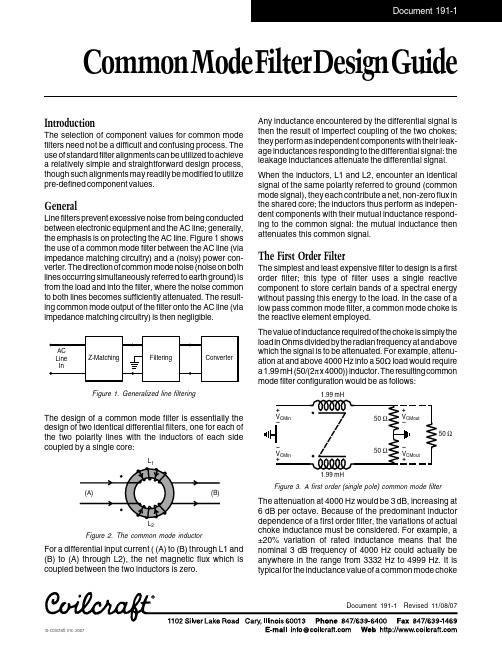
Common M ode F ilter D esign G uideIntroductionThe selection of component values for common mode filters need not be a difficult and confusing process. The use of standard filter alignments can be utilized to achieve a relatively simple and straightforward design process, though such alignments may readily be modified to utilize pre-defined component values.GeneralLine filters prevent excessive noise from being conducted between electronic equipment and the AC line; generally, the emphasis is on protecting the AC line. Figure 1 shows the use of a common mode filter between the AC line (via impedance matching circuitry) and a (noisy) power con-verter. The direction of common mode noise (noise on both lines occurring simultaneously referred to earth ground) is from the load and into the filter, where the noise common to both lines becomes sufficiently attenuated. The result-ing common mode output of the filter onto the AC line (via impedance matching circuitry) is then negligible.Figure 1.Generalized line filteringThe design of a common mode filter is essentially the design of two identical differential filters, one for each of the two polarity lines with the inductors of each side coupled by a single core:L2Figure 2.The common mode inductorFor a differential input current ( (A) to (B) through L1 and (B) to (A) through L2), the net magnetic flux which is coupled between the two inductors is zero.Any inductance encountered by the differential signal is then the result of imperfect coupling of the two chokes; they perform as independent components with their leak-age inductances responding to the differential signal: the leakage inductances attenuate the differential signal. When the inductors, L1 and L2, encounter an identical signal of the same polarity referred to ground (common mode signal), they each contribute a net, non-zero flux in the shared core; the inductors thus perform as indepen-dent components with their mutual inductance respond-ing to the common signal: the mutual inductance then attenuates this common signal.The First Order FilterThe simplest and least expensive filter to design is a first order filter; this type of filter uses a single reactive component to store certain bands of a spectral energy without passing this energy to the load. In the case of a low pass common mode filter, a common mode choke is the reactive element employed.The value of inductance required of the choke is simply the load in Ohms divided by the radian frequency at and above which the signal is to be attenuated. For example, attenu-ation at and above 4000 Hz into a 50⏲ load would require a 1.99 mH (50/(2π x 4000)) inductor. The resulting common mode filter configuration would be as follows:50Ω1.99 mHFigure 3.A first order (single pole) common mode filter The attenuation at 4000 Hz would be 3 dB, increasing at 6 dB per octave. Because of the predominant inductor dependence of a first order filter, the variations of actual choke inductance must be considered. For example, a ±20% variation of rated inductance means that the nominal 3 dB frequency of 4000 Hz could actually be anywhere in the range from 3332 Hz to 4999 Hz. It is typical for the inductance value of a common mode choketo be specified as a minimum requirement, thus insuring that the crossover frequency not be shifted too high.However, some care should be observed in choosing a choke for a first order low pass filter because a much higher than typical or minimum value of inductance may limit the choke’s useful band of attenuation.Second Order FiltersA second order filter uses two reactive components and has two advantages over the first order filter: 1) ideally, a second order filter provides 12 dB per octave attenuation (four times that of a first order filter) after the cutoff point,and 2) it provides greater attenuation at frequencies above inductor self-resonance (See Figure 4).One of the critical factors involved in the operation of higher order filters is the attenuating character at the corner frequency. Assuming tight coupling of the filter components and reasonable coupling of the choke itself (conditions we would expect to achieve), the gain near the cutoff point may be very large (several dB); moreover, the time response would be slow and oscillatory. On the other hand, the gain at the crossover point may also be less than the presumed -3 dB (3 dB attenuation), providing a good transient response, but frequency response near and below the corner frequency could be less than optimally flat.In the design of a second order filter, the damping factor (usually signified by the Greek letter zeta (ζ )) describes both the gain at the corner frequency and the time response of the filter. Figure (5) shows normalized plots of the gain versus frequency for various values of zeta.Figure 4.Analysis of a second order (two pole) common modelow pass filterThe design of a second order filter requires more care and analysis than a first order filter to obtain a suitable response near the cutoff point, but there is less concern needed at higher frequencies as previously mentioned.A ≡ ζ = 0.1;B ≡ ζ = 0.5;C ≡ ζ = 0.707;D ≡ ζ = 1.0;E ≡ ζ = 4.0Figure 5.Second order frequency response for variousdamping f actors (ζ)As the damping factor becomes smaller, the gain at the corner frequency becomes larger; the ideal limit for zero damping would be infinite gain. The inherent parasitics of real components reduce the gain expected from ideal components, but tailoring the frequency response within the few octaves of critical cutoff point is still effectively a function of ideal filter parameters (i.e., frequency, capaci-tance, inductance, resistance).L0.1W n1W n 10W nRadian Frequency,WG a i n (d B )V s V s LR s LCs LC j L R j LC LR LCCMout CMin L L n n n L ()()=++=−+⎛⎝⎜⎞⎠⎟=+−⎛⎝⎜⎞⎠⎟≡≡≡≡111111212222ωωζωωωωωωζradian frequencyR the noise load resistance LFor some types of filters, the design and damping char-acteristics may need to be maintained to meet specific performance requirements. For many actual line filters,however, a damping factor of approximately 1 or greater and a cutoff frequency within about an octave of the calculated ideal should provide suitable filtering.The following is an example of a second order low pass filter design:1)Identify the required cutoff frequency:For this example, suppose we have a switching power supply (for use in equipment covered by UL478) that is actually 24 dB noisier at 60 KH z than permissible for the intended application. For a second order filter (12dB/octave roll off) the desired corner frequency would be 15 KHz.2)Identify the load resistance at the cutoff frequency:Assume R L = 50 Ω3)Choose the desired damping factor:Choose a minimum of 0.707 which will provide 3 dB attenuation at the corner frequency while providing favorable control over filter ringing.4)Calculate required component values:Note:Damping factors much greater than 1 may causeunacceptably high attenuation of lower frequen-cies whereas a damping factor much less than 0.707 may cause undesired ringing and the filter may itself produce noise.Third Order FiltersA third order filter ideally yields an attenuation of 18 dB per octave above the cutoff point (or cutoff points if the three corner frequencies are not simultaneous); this is the prominently positive aspect of this higher order filter. The primary disadvantage is cost since three reactive compo-nents are now required. H igher than third order filters are generally cost-prohibitive.Figure 6.Analysis of a third order (three pole) low pass filter where ω1, ω2 and ω4 occur at the same -3dB frequency of ω05)Choose available components:C = 0.05 µF (Largest standard capacitor value that will meet leakage current requirements for UL478/CSA C22.2 No. 1: a 300% decrease from design)L = 2.1 mH (Approx. 300% larger than design to compensate for reduction or capacitance: Coilcraft standard part #E3493-A)6)Calculate actual frequency, damping factor, and at-tenuation for components chosen:ζ = 2.05 (a damping factor of about 1 or more is acceptible)Attenuation = (12 dB/octave) x 2 octaves = 24 dB 7)The resulting filter is that of figure (4) with:L = 2.1 mH; C = 0.05 µF; R L = 50 ΩL 1L 2VCMout s VCMin s R R L s R L s sC R L s sC R L s L L s L s sC L L R s L Cs L L C R s L L L L L L L()()()()=+⎛⎝⎜⎞⎠⎟+++++⎛⎝⎜⎜⎜⎜⎞⎠⎟⎟⎟⎟=++++222121*********11Butterworth →+++112212233s s s n n n ωωω()()L L R R L L L n n L 12111222+==+ωω;()L L C n 1n2C =2;ωω2211414=.L L L L n n n 12L n3n2L2n2L2C R =1;R R ωωωωωω33224422===ωπωζωμn n n Lf C L L R L =====294248070727502rad /sec =1Hn .1215532πLC=Hz (very nearly 15KHz)The design of a generic filter is readily accomplished by using standard alignments such as the Butterworth (“maxi-mally flat”) alignments. Figure (6) shows the general analysis and component relationships to the Butterworth alignments for a third order low pass filter. Butterworth alignments provide an inherent ζ of 0.707 and a -3 dB point at the crossover frequency. The Butterworth alignments for the first three orders of low pass filters are shown in Figure (7).The design of a line filter need not obey the Butterworth alignments precisely (although such alignments do pro-vide a good basis for design); moreover, because of leakage current limits placed upon electronic equipment (thus limiting the amount of filter capacitance to ground),adjustments to the alignments are usually required, but they can be executed very simply as follows:1)First design a second order low pass with ζ ≥ 0.52)Add a third pole (which has the desired corner fre-quency) by cascading a second inductor between the second order filter and the noise load:L = R/ (2 π f c )Where f c is the desired corner frequency.Design ProcedureThe following example determines the required compo-nent values for a third order filter (for the same require-ments as the previous second order design example).1)List the desired crossover frequency, load resistance:Choose f c = 15000 Hz Choose R L = 50 Ω2)Design a second order filter with ζ = 0.5 (see second order example above):3)Design the third pole:R L /(2πf c ) = L 250/(2π15000) = 0.531 mH4)Choose available components and check the resulting cutoff frequency and attenuation:L2 = 0.508 mH (Coilcraft #E3506-A)f n= R/(2πL 1 )= 15665 HzAttenuation at 60 KHZ: 24 dB (second order filter) +2.9 octave × 6 = 41.4 dB5)The resulting filter configuration is that of figure (6)with:L 1 = 2.1 mH L 2 = 0.508 mH R L = 50 ΩConclusionsSpecific filter alignments may be calculated by manipu-lating the transfer function coefficients (component val-ues) of a filter to achieve a specific damping factor.A step-by-step design procedure may utilize standard filter alignments, eliminating the need to calculate the damping factor directly for critical filtering. Line filters,with their unique requirements, yet non-critical character-istics, are easily designed using a minimum allowable damping factor.Standard filter alignments assume ideal filter compo-nents; this does not necessarily hold true, especially at higher frequencies. For a discussion of the non-ideal character of common mode filter inductors refer to the application note “Common Mode Filter Inductor Analysis,”available from Coilcraft.Figure 7.The first three order low pass filters and their Butterworth alignmentse i +–e O +–R LL 2Ce i +–e O +–R LL 1Ce i +–e O +–R LL 1L 2Filter SchematicFilter Transfer FunctionButterworthAlignmentFirst OrderSecond OrderThird Ordere e Ls R o iL =+11e e LCs Ls R oi L=++112e e L L R s L Cs L L s R o iLL =++++111231212()e e s o in=+11ωe e LCs Ls R oiL =++112e e s s so i n n n =+++122133221ωωω。

a r X i v :h e p -t h /0308094v 1 14 A u g 2003On the No-Go Theorem of Supersymmetry BreakingWung-Hong Huang*Department of PhysicsNational Cheng Kung UniversityTainan,70101,Taiwan ABSTRACT It is proved that,even if the gauge symmetry has been broken spontaneously at tree level,supersymmetry would never break through any finite orders of perturbation if it is not broken classically.*E-mail:whhwung@.twPhysics Letters B179(1986)92Supersymmetry[1],which is the only graded Lie algebra of symmetries of the S-matrix that is consistent with the relativistic quantumfield theory[2],could exhibit improved ultraviolet behavior[3,4]and provide us with a solution of the gauge hierarchy problem[5]. It has been shown that,in a broad class offield theories[6],if supersymmetry is not broken at the classical level then it is not broken by radiative corrections.Those are the models with only chiral superfields and models whose gauge symmetry and supersymmetry are unbroken classically.Recently Ovrut and Wess[7]have examined a class of supersymmetric theories whose internal symmetry is completely broken spontaneously.After extending the Rζgauge-fixing [8]procedure to the supersymmetric theories they calculated the one-loop corrections to the auxiliaryfields.It is found that the invariance of the superpotential under the complexifica-tion of the internal symmetry group allows the vacuum expectation values of scalarfields to be adjusted to make the corrected D terms vanish while keeping the F terms zero.Hence, the supersymmetry is not broken.In this paper,without explicitly calculating the quantum correction,we will prove that this another no-go theorem is always true in any supersym-metric gauge theory.Furthermore,the internal symmetry is allowed not to be spontaneously broken completely.To break the supersymmetry infinite orders of perturbation,one must get an expectation value of the F or Dfiing the supergraphic techniques[4]it can be easily seen that the Ffield does not give an expectation value if supersymmetry is unbroken at the classical level.Also,there is no induced expectation value of the D term if both gauge symmetry and supersymmetry are unbroken classically[9].In other words,the Coleman-Weinberg mecha-nism[10]is not possible.This is a no-go theorem that has been well established.When the gauge symmetry is already broken spontaneously at the classical level,quantum corrections for the D terms(but not F terms)are induced.In the following sections we shall show that, for any induced Dfield,through some suitable transformations of complexification of the internal symmetry group one can alwaysfind vacuum expectation values of the scalarfields to make the D terms vanish.(Recall that the superpotential is invariant under the complex-ified internal symmetry group so that the F terms remain zero.)Hence,supersymmetry isnot broken as claimed by Ovrut and Wess[7].Considerfirst the supersymmetric theory with abelian gauge symmetry group.Let Φ+i,Φ−j,andΦ0k be chiral superfields with positive charge q+i,negative charge q−j and zero charge,respectively.In order to preserve the supersymmetry in the n-th order of per-turbation,there must exist the vacuum expectation values a(n)+i,a(n)−j and a(n)0k of scalarfields in the chiral superfields,Φ+i,Φ−j,andΦ0k,which satisfyi q+i|a(n)+i|2+ j q−j|a(n)−j|2=C(n)(a(n)+i,a(n)−j,a(n)0k),(1) where the functional form of C(n)depends on the order of perturbation.At tree level,the C(n)term does not show up.After the quantum correction,it is induced.Tofind the solution of(1)we set,in the spirit of perturbation theory,the values of a(n)+i,a(n)−j,and a(n)0k in the argument of the function C(n)to the(n−1)th order only and the equation which we need to solve becomesi q+i|a(n)+i|2+ j q−j|a(n)−j|2=C(n)(a(n−1)+i,a(n−1)−j,a(n−1)0k),(2)The existence of a solution for the above equation can be proved by the following observa-tions.First,when the gauge group is already broken classically then there must exist at least one nonzero vacuum expectation value among,a(0)+i or a(0)−j which satisfiesi q+i|a(0)+i|2+ j q−j|a(0)−j|2=0.(3) Furthermore,because q+i is positive while q−j is negative,there must exist at least one nonzero value a(0)+i accompanied with at least one nonzero value a(0)+i in order to satisfy the above equation.Next,consider the one-loop correction.We see that the C(1)term is only a function of tree-level vacuum expectation values,so it can be regarded as afixed number when we want tofind the one-loop vacuum expectation values a(1)+i,a(1)−j,a(1)0k which satisfy eq.(2).Therefore,regardless of the value of C(1),it is easily seen that we can alwaysfind a real parameterθsuch that a(1)+i and a(1)−j,which we are searching now,are just the transformed values of a(0)+i and a(0)−j under the complexified internal symmetry group,i.e.a(1)+i=a(0)+i exp(q+iθ),a(1)−j=a(0)−j exp(q−jθ).(4) For example,if C(1)is positive(negative)thenθmust be positive(negative).The point is that there exists at least one nonzero value a(0)+i accompanied with at1east one nonzero value a(0)−j.For higher loop corrections,the above discussion can still be used.We next examine supersymmetric theories with non-abelian internal symmetry which is broken spontaneously.But the complete breaking is not necessary.Let Tαbe the generators of the gauge group and the chiral superfieldΦbe its representation.(Extension to many different representations is straightforward.)The vacuum expectation value of the scalar field inΦis denoted as a.To preserve the supersymmetry in the n th order of perturbation there must exist an a(n)to satisfya(n)†Tαa(n)=C(n)α(a(n)),(5) where the functional form of C(n)αdepends on the order of the perturbation.In the spirit of perturbation theory,as in the abelian case,we let a(n)in the argument of C(n)αbe a(n−l) and(5)becomesa(n)†Tαa(n)=C(n)α(a(n−1)),(6) To solve a(n)in the above equation we can regard a(n−l)asfixed ing this property,we prove that there always exists a solution a(n)which satisfies(6)regardless of the value of C(n)αwhich depends on the model and the order of perturbation.Hence, supersymmetry is not broken through quantum corrections.Consider a system whose gauge symmetry has been spontaneously broken at tree level; there exists at least a generator T r which satisfiesT r a(0)=0,(7)where T r belongs to the Cartan subalgebra with diagonal elements only,i.e.=t r iδij.(8)T rijEq.(7)then tells us that there must exist at least one nonzero value t r i a(0)i.Also,eq.(6) becomesa(0)†T r a(0)= i t r i|a(0)i|2=0.(9)This shows that there must exist at least one positive and one negative value among t r i|a(0)i|2.If we rotate a(0)in Cartan subspace of the complexified internal symmetry group1a(0)→a(0)exp(,(11)2 r t r iθrthen it is obvious that the slopes of L(θr)are just a(0)′†T r a(0)′and can take on any value.It is this property that,no matter what the value of α|C(n)α|2,we can alwaysfind a set of θr to satisfyα|a(0)′†T r a(0)′|2= α|C(n)α|2.12) Finally,with the fact that the a(0)′†T r a(0)′are transformed as vectors in the regular representation of the internal symmetry group,we can rotate them to satisfy(6).Therefore, the solution of(6)is found and supersymmetry is still preserved at the quantum level.REFERENCES1.J.Wess and B.Zumino,Nucl.Phys.B70(1974)39.2.R.Hagg,J.Lopuszanski and M.Sohnius,Nucl.Phys.B88(1975)257.3.J.Wess and B.Zumino,Phys.Lett.B49(1974)52;J.Iliopoulos and B.Zumino,Nucl.Phys.B79(1974)310.4.M.T.Grisaru,W.Siegel and M.Rocek,Nucl.Phys.B159(1979)429.5.E.Witten,Phys.Lett.B105(1981)267.6.B.Zumino,Nucl.Phys.B89(1975)535;ng,Nucl.Phys.B114(1976)123;S.Weinberg,Phys.Lett.B62(1976)111.7.B.A.Ovrut and J.Wess,Phys.Rev.D25(1982)409.8.K.Fujikawa,B.W.Lee and A.I.Sanda,Phys.Rev.D6(1972)2923.9.E.Witten,Nucl.Phys.B185(1981)513.10.S.Coleman and E.Weinberg,Phys.Rev.D7(1973)888.。