网络分析仪校准步骤

EC网络分析仪测试方法EC网络分析仪是一种用于测试电子设备和电路的仪器，能够精确地测量电路的电气性能和信号传输特性。

在使用EC网络分析仪进行测试时，需要遵循一定的测试方法和步骤，以确保测试结果的准确性和可靠性。

下面是EC网络分析仪测试方法的详细步骤：1.准备工作在进行测试之前，首先需要准备好EC网络分析仪及其相关测试配件，如测试夹具、连接线等。

确保所有设备都处于正常工作状态，并进行必要的校准和调试。

2.连接测试设备将待测试的电路或设备连接到EC网络分析仪上，确保连接线路的质量和稳定性。

在连接过程中，应避免产生干扰或杂音，以确保测试结果的准确性。

3.设置测试参数在EC网络分析仪上设置所需的测试参数，包括频率范围、功率水平、扫描速度等。

根据测试对象的特性和需求，调整相应的参数以实现最佳的测试效果。

4.进行预测试进行预测试以验证连接和设置是否正确，以及测试系统是否正常工作。

可以使用标准件或校准器件进行校准和验证，以确保测试结果的准确性和可靠性。

5.进行主要测试在确认预测试结果正常后，进行主要的测试过程。

根据测试要求和目的，选择适当的测试模式和方法，如频率扫描、功率扫描、时域测试等。

记录和保存测试数据，以备后续分析和比较。

6.分析测试结果对测试数据进行分析和处理，提取所需的电气参数和特性，并进行图表化展示和比较。

可以使用EC网络分析仪软件进行数据处理和分析，以实现更精确和全面的测试结果。

7.解释测试结果根据分析得到的测试结果，进行合理的解释和说明，评估电路或设备的性能和可靠性。

根据测试结果，制定相应的改进方案或措施，以优化电路设计和性能。

8.撰写测试报告根据测试过程和结果，撰写详细的测试报告，包括测试方法、参数设置、数据分析和结论等内容。

报告应清晰明了，具有可操作性和可复现性，以满足相关标准和要求。

9.完成测试和总结完成测试过程后，对测试过程和结果进行总结和回顾，总结经验和教训，提出改进建议和建议。

对测试设备进行清洁和维护，以确保下次测试的准确性和可靠性。

VNA使用方法:矢量网络分析仪校
是不是每次测量一个新的项目前都必须做校准?
这个是不一定需要的，尽量将每次校准的state存入VNA，名字最好为校准状态，例如频率范围，输入激励功率等。

如果有新的测试项目，但是它的测试条件和已有状态相似，且load state后，检查校准状态良好，就可用使用以前的校准状态，而不需要重新校准。

将校准state保存并调用的好处在于：CalibraTIon Kit也是有使用寿命的，多次的校准，会是的校准件多次和校准电缆接触，可能污染校准件，使得校准件特性发生改变，影响下一次校准。

尽量养成如下习惯：将网络分析仪的port不用的时候加上防尘套;对测试电缆进行标号，使得VNA每个port尽可能固定连接某个电缆;对测试电缆不用时，也需要加上防尘套;尽量不用很脏的测试电缆等。

网络分析仪基本操作介绍一、概述随着信息技术的飞速发展，网络已成为现代生活和工作中不可或缺的一部分。

为了更好地分析和优化网络性能，网络分析仪作为一种重要的测试工具被广泛应用。

网络分析仪基本操作介绍对于使用者来说至关重要，本文将详细介绍网络分析仪的基本操作，帮助读者更好地理解和使用这一强大的工具。

网络分析仪主要用于测量网络中的各项参数，如信号的频率响应、失真度、噪声系数等，以评估网络性能。

通过掌握网络分析仪的基本操作，使用者可以准确地分析网络中的各种问题，并找到相应的解决方案。

本文旨在让读者了解网络分析仪的基本功能、操作方法和使用注意事项，以便在实际应用中能够准确、高效地使用网络分析仪。

1. 介绍网络分析仪的重要性和应用领域随着互联网技术的飞速发展和信息通信技术的日益成熟，网络已经成为了我们日常生活与工作中不可或缺的重要部分。

为了确保网络的稳定、高效和安全运行，网络分析仪成为了必不可少的重要工具。

因此本文将为大家介绍网络分析仪的基本操作，本文将重点阐述的第一部分，是关于网络分析仪的重要性和应用领域。

在当今信息化社会，网络已经渗透到各行各业和千家万户的日常生活中。

无论是企业级的复杂网络系统，还是家庭用户的日常网络连接，网络的性能优化和故障排查成为了保证业务连续性和生活质量的关键环节。

网络分析仪在这一点上发挥着至关重要的作用，它可以对网络信号进行捕捉、分析和可视化处理，帮助工程师和IT专家迅速定位网络问题，提供准确的数据分析和解决方案。

因此网络分析仪是维护网络正常运行、提升网络性能的关键工具。

网络分析仪的应用领域非常广泛，几乎涵盖了所有涉及网络通信的领域。

以下列举几个主要应用领域：通信行业：在网络规划、部署和维护阶段，网络分析仪用于测试和优化无线和有线通信网络。

通过对信号质量的精确分析，确保通信的稳定和高效。

网络安全领域：网络分析仪通过深度分析网络流量和行为模式，有助于发现潜在的安全威胁，帮助防御各种网络安全攻击。

5.1 按键区域123 645 78软选择（可根据自己Loss compen：损耗修正设定菜单；Sensor A setting：设定通道A的功率传感器校准系数；Sensor B setting：设定通道B的功率传感器校准系数；Return：返回。

11.8 Calibration(校准设定)Start：设置频段的起始位置；Stop：设置频段的终止位置；Center：设置频段的中心位置；Spen：设置频段范围。

11.10 Sweep setup(扫描设置)Power：打开激励信号输出设置菜单；Power：设置网络分析仪内部信号源的输出功率电平；Power renges：选择功率电平范围；Auto ranges：将功率电平范围设置为自动选择；Port couple：是否在现有电平上打开端口耦合；Port power：当端口耦合关闭时设置端口功率；CW freq：设置功率扫描的固定频率；Rf out：是否打开激励源的输出开关；Return：返回。

Sweep time：设置端口扫描时间；Sweep delay：设置端口扫描延时；Sweep mode：选择扫描模式Std stepped：略；Std swept：略；Fast stepped：略；Fast swept：略；Points：设置每次扫描时的扫描点数；Marker→ref maker：将当前被缴活的Marker点设为参考Marker点；Ref marker mode：设置为参考标记模式；Return：返回。

11.13 Marker search(标记搜索)Max：将Marker点移动到当前轨迹上的最大点；Min：将Marker点移动到当前轨迹上的最小点；Peak：峰值功能；Search peak：寻找顶峰；Search left：在左侧寻找顶峰；Search rifht：在右侧寻找顶峰；Peak excursion：设置顶峰偏移；Peak polarity：极性设置；Positive：正极性；Negative：负极性；Both：双极性；Cancel：取消；Return：返回。

矢量网络分析仪使用说明书第一章前言1. E836B网络分析仪具有以下技术特点：①高性能测量接收机E8362A网络分析仪采用基于混频器的实现方式，使该仪表具有当今微波网络分析仪中最高的测量灵敏度度。

测量频率范围：10M~20GHz;接收机数量：4台接收机测量灵敏度：-120dBm接收机测量参数；幅度和相位。

迹线噪声：0.005dB(在中频带宽为10KHz时)②完整的测量能力该网络分析可以工作在以下测量状态：频域扫描状态：测量激励信号为功率固定，频率变化信号。

考察被测在不同频率激励状态下等离子参数的变化；功率扫描状态：测量激励信号为频率固定，功率扫描变化信号。

考察被测在不同功率激励状态下参数的变化；连续波状态：测量激励信号为频率固定，功率固定信号。

考察被测等离子在固定激励状态下，响应状态参数的波动变化，E8362A最大测量时间长度可达到3000秒；时间域测量状态：通过将被测的频率响应通过IFFT变化到时间域得到其时域冲击响应，考察被测等离子响应信号的空中分布特性。

E8362AIFFT运算点数为160001点，可保证时域测量的分辨率和测量时间宽度。

③强大的分析能力E8362A基于PC的window2000操作平台，可内置各种分析软件，不需要外置PC 进行数据处理，编程方式为COM/DCOM，保证测试的速度。

仪表内置嵌入、去嵌入及端口延伸等功能，可直接消除测量天线对测量结果的影响，或进行其它补偿运算处理。

④高测量速度E8262A高性能接收机可确保高测量精度的同时具有快测量速度，具体指标为：35us/测量点，14ms/刷新（400点）。

保证对被测等离子的瞬态响应进行捕捉分析。

⑤多测试状态同时完成E8262A可支持16个测试通道，各通道可工作在不同的测量状态。

利用该功能，可以综合不同分析方法从不同角度来对一个现象进行研究。

⑥良好的可扩展性E8263A采用开放的发射/接收组成框架，用户可以根据测量的具体要求改变仪表的测量连接状态，还可以把需要的外部信号处理过程组合到仪表内部，例如：当被测需要更大激励功率时，可将推动方法器连接到仪表相应端口，该放大器引起的测试误差可以通过仪表的校准过程消除。

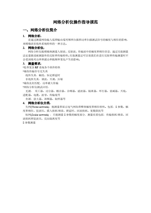
网络分析仪操作指导规范一、网络分析仪简介1.网络分析：是通过测量网络输入端和输出端对频率扫描和功率扫描测试信号的幅度与相位的影响，来精确表征线性系统特性的一种方法。

2.网络分析仪：网络分析仪能精确地测量入射波、反射波、传输波中的幅度和相位信息，通过比值测量法定量描述被测器件的反射和传输特性。

比值测量法可以使我们在进行反射和传输测量时不会受到绝对功率和源功率随频率变化产生的影响。

3.测量需求：•检查复杂RF系统各个组件特性•确保传输信号无失真线性失真：幅度、恒定群延时非线性失真：谐波、互调、压缩•确保良好匹配，功率最大传输•网络分析仪测试应用：无源：双工器、功分器、耦合器、合路器、滤波器、隔离器、环行器、衰减器、天线、适配器、电缆、波导、传输线等有源：放大器、混频器、取样器等4.网络分析仪分类：矢网(V ector network)：能测量和显示电气网络和整体幅度和相位特性。

包括：S参数、幅度和相位、驻波比、插入损耗/增益、群延时、回波损耗、复数阻抗等标网(Scalar network) ：只能测量S参数的幅度部分，测量结果包括：传输损耗/增益、回波损耗和驻波比、反向隔离度等S参数测量5.测试误差分析：测量系统存在误差：•系统误差：是由测试设备和测量装置的不完善所引起•随机误差：以随机方式随时间而变，不可通过校准来消除。

主要影响：噪声、开关重复性、连接重复性。

•漂移误差：频率漂移、温度漂移6.网络分析仪系统误差：系统误差为主要误差，可通过校准消除。

存在6种类型12个误差项：•与信号泄漏有关的方向误差和串扰误差•与反射有关的源失匹配和负载阻抗失配；•由反射和传输跟踪引起的频率响应误差7.误差修正：网络分析仪的测量准确度受外部因素的影响较大。

误差修正是提高测量准确度的过程。

误差修正是对已知校准标准进行测量，将这些测量结果贮存到分析仪的存储器内，利用这些数据来计算误差模型。

然后，利用误差模型从后续测量中去除系统误差的影响。

矢量网络分析仪的误差分析和处理一、矢量网络分析仪的误差来源矢量网络分析仪的测量的误差主要有漂移误差、随机误差、系统误差这三大种类。

1、漂移误差漂移误差是由于进行校准之后仪器或测试系统性能发生变化所引起，主要由测试装置内部互连电缆的热膨胀特性以及微波变频器的变换稳定性引起,且可以通过重新校准来消除.校准维持精确的时间范围取决于在测试环境下测试系统所经受到的漂移速率。

通常,提供稳定的环境温度便能将漂移减至最小。

2、随机误差随机误差是不可预测的且不能通过误差予以消除，然而，有若干可以将其对测量精度的影响减至最小的方法，以下是随机误差的三个主要来源：（1）仪器噪声误差噪声是分析仪元件中产生的不希望的电扰动。

这些扰动包括：接收机的宽带本底噪声引起的低电平噪声；测试装置内部本振源的本底噪声和相位噪声引起的高电平噪声或迹线数据抖动。

可以通过采取以下一种或多种措施来减小噪声误差:提高馈至被测装置的源功率；减小中频带宽；应用多次测量扫描平均.1（2）开关重复性误差分析仪中使用了用来转换源衰减器设置的机械射频开关。

有时，机械射频开关动作时，触点的闭合不同于其上次动作的闭合。

在分析仪内部出现这种情况时,便会严重影响测量的精度。

在关键性测量期间，避免转换衰减器设置，可以减小开关重复性误差的影响。

(3）连接器重复性误差连接器的磨损会改变电性能。

可以通过实施良好的连接器维护方法来减小连接器的重复性误差。

3、系统误差系统误差是由分析仪和测试装置中的不完善性所引起。

系统误差是重复误差（因而可预测），且假定不随时间变化，可以在校准过程中加以确定，且可以在测量期间用数学方法减小。

系统误差决不能完全消除，由于校准过程的局限性而总是存在某些残余误差，残余(测量校准后的）系统误差来自下列因素：校准标准的不完善性、连接器界面、互连电缆、仪表.反射测量产生下列三项系统误差：方向性、源匹配、频率响应反射跟踪。

传输测量产生下列三项系统误差：隔离、负载匹配、频率响应传输跟踪。

矢量网络分析仪操作规程
1、测量前准备
打开电源，让仪器预热30分钟,将标准同轴线接于仪器上,同时准备好用于校准的标准件。

按下Preset键,进行网络分析仪初始化面板的预设。

2、测量前校准
在首次操作仪器之前或每隔一个月或根据仪器的使用情况，必须对网络分析仪进行校准。

为使测量结果更为精确，必须分别连接开路、短路、负载设备进行校准。

用户可以对校准后的数据进行保存，开机时可直接调用，而不需要设置和校准。

3、开始实验
确保操作本仪器的任何人员已接受过实验室一般安全操作规程和本仪器特别安全操作规程的培训与指导。

根据测量的设备，依次进行中频带宽的设定，测量轨迹的设定，扫频方式的设定，起始和终止频率的设定，Marker读值的设定。

测量完毕后对需要保存的数据和图形进行存储操作，以便下次直接调用。

4、关闭网络分析仪
测试完毕后关闭系统，点击System>Exit，进入Windows XP界面，之后关闭计算机。

矢量网络分析仪使用教程矢量网络分析仪（Vector Network Analyzer，简称VNA）是一种用于测量和分析电磁网络参数的高精度仪器。

它主要用于测试和优化射频和微波器件的性能，如天线、滤波器、放大器、集成电路等。

本文将为您提供一份针对矢量网络分析仪的使用教程，帮助您快速上手使用该仪器。

一、仪器介绍矢量网络分析仪是一种精密仪器，主要由信号源、接收器和调制器等组成。

它能够通过在被测设备上施加相应的输入信号，并测量输出信号的幅度和相位，从而计算出设备的散射参数（S-parameters）。

矢量网络分析仪通常具有高精度、宽频率范围和高灵敏度等特点，能够提供准确的测量结果。

二、基本操作1. 连接被测设备：首先，将矢量网络分析仪的输出端口与被测设备的输入端口连接，确保连接牢固。

如果被测设备具有多个端口，需要逐个连接。

2. 仪器校准：在测量之前，需要对矢量网络分析仪进行校准，以确保测量结果的准确性。

通常有三种常见的校准方法：全开路校准、全短路校准和全负载校准。

具体的校准方法可以根据被测设备的性质和实际需求进行选择。

3. 设置测量参数：在测量之前，需要设置一些测量参数，如频率范围、功率级别、测量类型等。

这些参数可以根据被测设备的特性和实际需求进行调整。

4. 启动测量：配置好测量参数后，可以开始进行测量。

在测量过程中，矢量网络分析仪会自动控制信号源和接收器，并采集输入和输出信号的数据。

5. 数据分析：测量完成后，可以通过矢量网络分析仪的软件对测量数据进行分析和处理。

常见的数据处理操作包括绘制频率响应图、计算散射参数、优化器件设计等。

三、注意事项1. 确保连接正确：在使用矢量网络分析仪进行测量前，需要确保所有连接正确无误，以避免测量误差的发生。

同时，还需要确保连接的电缆和连接器的质量良好，以减小测量误差。

2. 避免干扰源：在进行测量时，需要避免与其他无关信号源相互干扰，如电源噪音、射频噪声等。

可以通过在实验室中采取屏蔽措施来减小干扰。

网络分析仪试题及答案一、单项选择题（每题 2 分，共 10 题）1. 网络分析仪的主要功能是什么？A. 测量电阻B. 测量电压C. 测量网络的反射和传输参数D. 测量电流2. 网络分析仪的S参数中，S11代表什么？A. 输入反射系数B. 输出反射系数C. 隔离度D. 增益3. 网络分析仪的频率范围通常是多少？A. 100kHz - 1GHzB. 1MHz - 20GHzC. 100MHz - 40GHzD. 1GHz - 50GHz4. 网络分析仪的动态范围是指什么？A. 最大测量值与最小测量值的比值B. 最大测量值与最小测量值的差值C. 最大测量值与平均测量值的比值D. 最小测量值与平均测量值的差值5. 网络分析仪的校准通常包括哪些步骤？A. 仅开路校准B. 仅短路校准C. 开路、短路和负载校准D. 开路、短路和反射校准6. 网络分析仪的测量精度受哪些因素影响？A. 温度和湿度B. 电源电压C. 操作者的技术水平D. 所有上述因素7. 网络分析仪的测量误差通常包括哪些类型？A. 系统误差和随机误差B. 系统误差和操作误差C. 随机误差和操作误差D. 系统误差、随机误差和操作误差8. 网络分析仪的测量结果通常以哪种格式显示？A. 表格B. 图形C. 文本D. 音频9. 网络分析仪的测量速度与哪些因素有关？A. 测量点的数量B. 仪器的硬件性能C. 被测网络的复杂度D. 所有上述因素10. 网络分析仪的测量结果可以通过哪种方式进行验证？A. 人工计算B. 与其他仪器对比C. 重复测量D. 所有上述方式答案：1. C2. A3. B4. A5. C6. D7. D8. B9. D10. D二、多项选择题（每题 2 分，共 10 题）1. 网络分析仪可以测量哪些参数？A. 阻抗B. 增益C. 群延迟D. 相位2. 网络分析仪的S参数中，S21代表什么？A. 正向增益B. 反向增益C. 正向传输系数D. 反向传输系数3. 网络分析仪的校准方式包括哪些？A. 单端口校准B. 双端口校准C. 多端口校准D. 全端口校准4. 网络分析仪的测量误差来源可能包括哪些？A. 仪器误差B. 连接线误差C. 接触不良D. 环境因素5. 网络分析仪的测量结果可以通过哪些方式进行分析？A. 频域分析B. 时域分析C. 相位分析D. 群延迟分析6. 网络分析仪的测量速度受哪些因素影响？A. 测量点的数量B. 仪器的硬件性能C. 被测网络的复杂度D. 操作者的技能7. 网络分析仪的测量误差可以通过哪些方式减少？A. 校准B. 使用高质量的连接线C. 确保良好的接触D. 控制环境因素8. 网络分析仪的测量结果可以通过哪些方式进行验证？A. 人工计算B. 与其他仪器对比C. 重复测量D. 使用标准件9. 网络分析仪的测量结果通常以哪些格式显示？A. 表格B. 图形C. 文本D. 音频10. 网络分析仪的测量结果可以用于哪些目的？A. 设计优化B. 故障诊断C. 性能验证D. 教学演示答案：1. A, B, C, D2. A, C3. A, B, C, D4. A, B, C, D5. A, B, D6. A, B, C, D7. A, B, C, D8. A, B, C, D9. A, B, C10. A, B, C, D三、判断题（每题 2 分，共 10 题）1. 网络分析仪可以测量网络的反射系数和传输系数。

矢量网络分析的校准:SOLT、TRL与Ecal作者：Louisu与以往的矢量网络分析仪(VNA)相比，现在的许多仪器提供了更多的校准方法供用户选择。

更多的选择固然好，但同时也带来了更多的混乱。

幸运的是，一些关键的比较点可以快速缩小选择范围，并确定最适当的校准技术。

本文将讨论常用的网络分析仪校准技术及其相对精度，重点是可靠的测量实践和其他能够改善精度的因素。

校准类型现在的网络分析仪都具有极强的处理能力和灵活性，针对特定应用的许多校准方法也随之涌现出来。

例如，针对特定应用的校准类型有混频器/变频器校准（用于频率偏置器件）、噪声系数校准和夹具内测量等。

下面以全面的1端口和2端口矢量校准为讨论的重点，并回顾网络分析仪中针对所有误差源的矢量校准方法。

这些方法与那些不考虑所有误差项的方法（例如响应校准）相比，精确度要高得多。

讨论校准精度时，将讨论范围限定为一些常用的校准类型，大多数现代校准方法来源于这些常用的校准类型。

常用的校准技术有三种：SOLT（短路－开路－负载－直通）、TRL（直通－反射－线路）和ECal（电子校准）模块。

在每一种校准技术中，通常又针对特定的测量要求（如宽带频率或晶圆上探测）分成不同的校准方法。

表1中总结了这些常用的校准技术及其各自的主要优势。

网络分析仪中的系统误差图1总结了典型网络分析仪中的系统误差来源。

相位测量功能使得VNA能够精确地计算所有的误差来源。

方向误差会影响反射测量的精度。

隔离误差会影响发射测量的精度。

源和负载误差与被测件和分析仪测量端口阻抗之间的失配有关。

反射和发射跟踪误差与分析仪的参考接收机和测量接收机的频率响应差异有关。

探究SOLT校准大多数网络分析仪用户最先熟悉的校准方法是SOLT。

SOLT校准能够提供优异的精度和可重复性。

这种校准方法要求使用短路、开路和负载标准校准件。

如果被测件上有雌雄连接器，还需要分别为雌雄连接提供对应的标准件，连接两个测量平面，形成直通连接。

使用网络分析仪进行波导校准件设置指南
 概述
 作为射频和微波测试的重要接插件和端口的类型，波导的应用领域十分广泛。

在矢量网络分析仪的测试应用当中，波导接口，尤其是矩形波导类型是常见接口之一。

 矢量网络分析仪的校准，是保证测试准确度的前提和必要条件。

本文主要阐述罗德与施瓦茨（R&S）矢量网络分析仪，在应用波导端口时，校准件参数的导入方法以及校准中的注意事项。

 矩形波导
 矩形波导的截止频率fc＝149.9/a （GHz）
 常见矩形波导参数。

屏幕区域：元件的名称和功能通道窗口用于显示迹线的窗口。

因为一个通道对应于一个窗口，所以称之为通道窗口。

通道窗口的外框显示为浅灰色时，通道为工作通道（正在为该通道执行设置）。

在下图中，通道 1（上方窗口）为工作通道。

要使通道成为工作通道，请使用“Channel Next”（下一通道）或“Channel Previous”（上一通道）键。

在通道窗口内部单击也可使通道成为工作通道。

通道 1 窗口通道 2 窗口5-1. 通道标题栏可以为每个通道分配标题，并将标题显示在标题栏上。

有关设置通道标题栏的更多信息，请参见为窗口添加标记。

5-2. 迹线名/测量参数此处显示了通道上迹线的名称（Tr1 至 Tr9）及其测量参数。

迹线名右侧的指示该迹线为工作迹线（正在为该迹线执行设置）。

要使迹线成为工作迹线，请使用“Trace Next”（下一迹线）或“Trace Prev”（上一迹线）键。

单击迹线名所在的线（鼠标指针从更改为）也可使迹线成为工作迹线。

5-3. 数据格式此处显示了每条迹线的数据格式。

有关设置数据格式的更多信息，请参见选择数据格式。

5-4. 刻度设置此处显示了每条迹线的刻度设置。

本示例说明“10.00dB/”对应每分度 10 dB。

“Ref 0.000dB”说明参考线的值为0 dB。

有关设置刻度的更多信息，请参见设置刻度。

5-5. 迹线状态区域此处显示了每条迹线的设置。

迹线状态显示属性名描述校准属性显示在每个通道上获取的校准系数的状态。

有关详细信息，请参见每个通道的校准系数采集状态。

E5091A 属性显示在每个通道上分配测试端口的信息。

有关详细信息，请参见显示 E5091A 属性。

平衡测量布局属显示每个通道上平衡测量的布局。

有关详细信息，请参见检查设备类型和端口分配。

性! 正在测量。

扫描时间超过 1.5 秒时，↑ 将显示在迹线的点上。

#（无显示）无效迹线。

测量条件已更改，但当前显示的通道上的迹线未更新为与新条件相符合的迹线。

如何利用矢量网络分析仪测量电缆阻抗和损耗第一步：校准。

除了待测电缆外，还需要另外一条辅助电缆。

我们使用的ZVB8矢量网络分析仪（下文中称矢网）有两个端口：Port1和Port2，测试前需先对这两个端口和辅助电缆进行校准，让矢网自动计算补偿值和进行错误校正。

步骤：1.矢网上电，将辅助电缆一端连接到一个端口，假设连到Port1。

2.取出calibration kit。

calibration kit有三个校准件：匹配器，短路器和开路器。

3.按矢网面板上CHANNEL组内的按钮（如图所示），打开校准菜单：4.在矢网屏幕右侧显示的菜单中依次点选菜单Start Cal->Two-Port P1P2->TOSM打开校准对话框（如图所示）：5.用NA VIGA TION组的和按钮移动焦点，用此组的和移动光标。

配合进行确定操作。

6.选择所用的Calibration Kit（我们使用的是“ZV-Z32 typical”）和Connector类型（我们使用“(f)”），然后按。

7.在接下来出现的对话框中（如图所示），将光标移动到某一行上，在辅助电缆的另一端接上相应的校准件，按测量，屏幕右侧会显示扫描出的绿色曲线。

（“Port1”表示在Port1上，即辅助电缆另一端上连接校准件；“Port2”表示在Port2上连接；“Through”表示将辅助电缆的另一端连到Port2上）扫描完成后，矢网会发“吡”的一声提示。

同时选定行左边会被打勾。

8.选定另一行，按同样的方法重复操作，直至所有行都被打上勾。

按。

校准完成。

第二步，测量电缆损耗。

1.将待测电缆连接于辅助电缆与Port2之间，然后按下矢网面板TRACE组内（如图所示）的按钮。

2.从矢网屏幕内右侧的菜单选择“S21”或“S12”，然后按下按钮右边的按钮（如上图图所示），从矢网屏幕内右侧的菜单选择“dB Mag”。

3.此时屏幕内出现曲线即为待测电缆在不同频率下得的衰减曲线。

AutoKal Automatic CalibrationofVector Network AnalyzerZVRbyHans-Gerd KrekelsRuhr-University BochumApplication Note 1EZ30_2E30 August 1996, Hans-Gerd Krekels, Ruhr-University BochumProducts:ZVR incl. Option ZVR-B1ZVRE incl. Option ZVR-B1Contents1.Introduction (2)1.1 Error Model of Network Analyzers (2)1.2 Manual Calibration Procedures (4)2. The AutoKal Procedure (5)2.1 Theoretical Description (6)2.1.1 Fundamental Calibration (8)2.1.2 Automatic Calibration (9)2.2 AutoKal for Analyzers with three Receiver Channels (9)3. Practical Realization and Application of the AutoKal Procedure (11)3.1 Realization of the Switching Unit (11)3.2 Implementation of the AutoKal Procedure (12)4. References (12)5. Further Application Notes (13)6. Ordering Information (13)1. IntroductionVector network analyzers are used in high frequency applications to measure the complex scattering parameters of an unknown device-under-test (DUT). In general, the DUT characteristics can be evaluated by using electromagnetic waves. The correlation between the incident, reflected and transmitted wave quantities at the DUT is defined by its scattering matrix S .Figure 1: Scattering parameter description of a two-port device.For a two-port DUT (Fig. 1), the scattering parameters have the following meaning:S 11: Reflection at port 1 with port 2 matchedS 21: Forward transmission with port 2 matchedS 12: Reverse transmission with port 1 matchedS 22: Reflection at port 2 with port 1 matchedSince network analyzers which measure the wave quantities a i , b i (i = 1, 2) are no ideal measuring instruments, the determination of the required scattering parameters is subject to errors. A significant enhancement of measurement accuracy, however, is possible by utilizing appropriate mathematical system error correction procedures. Therefore the non-ideal characteristics of the network analyzer must be known. The determination of these non-ideal characteristics can be performed by using a calibration procedure.1.1 Error Model of Network AnalyzersA block diagram of a vector network analyzer equipped with four receiver channels, e.g. ZVR, is shown in Fig. 2.Figure 2: Block diagram of a vector network analyzer, e.g. ZVRThe analyzer consists of a test set switch (SPDT switch) and two reflectometers G and H as well as four receiver channels m i (i = 1...4). The block DUT represents a device-under-test located between the two test ports.The correlation between the wave quantities a i , b i at the test ports and the measurement values m i is given by two error two-ports as described by the matrices G and H (Eq. 1) according to a four-port /two-port reduction [1]. The calculation of these two matrices is the task of the calibration procedure.b a G G G G m m a b H H H H m m 1111122122122211122122341 = = ;.()Besides the description of a DUT by scattering parameters, characterization with transmission matrices is also possible. The transmission matrix N is defined by a linear combination of the transmitted and reflected waves, however, in a different relationship. For a two-port, Eq. 2 is valid.b a N N N N a b S S S 111112212222211122112 = =−− ;det().N S ()A combination of Eq. 1 and Eq. 2 leads to the expression:m m m m 121343 = −G N H ()The block diagram of Fig. 2 reduces to a cascaded network consisting of two error two-ports and the DUT.Figure 3: Cascaded network of two error two-ports and the device-under-test.2 4The elimination of the waves a i , b i (i = 1, 2) in Eq. 1 by application of the scattering parameters yields the vector equation:G m G m H m H m S S S S G m G m H m H m 111122213224111221222112221131244++ = ++ ()A second vector expression is derived for the second position of the test set switch. If the measure-ment values of the second switch position are defined by m’ i (i = 1...4), a combination of the two vec-tor equations yields the matrix expression:S =G m G m G m G m H m H m H m H m G m G m G m G m H m H m H m H m 11112211112221322421322421122221122211312411312415++++ ++++ −’’’’’’’’()This expression can be used during calibration of the network analyzer. Moreover, the transformation of Eq. 5 for a known scattering matrix S results in four linear, independent equations which are useful during the calculation of the error parameters contained in the matrices G and H .A determination of the scattering matrix for an unknown DUT can also be performed with Eq. 5 if thesystem errors of the network analyzer are known.1.2 Manual Calibration ProceduresCommonly used procedures for the calibration of vector network analyzers, e. g. TOM or TRM [2] (T =Through, M = Match, O = Open, R = Reflect) are based upon the measurement of various known or partially unknown calibration standards. Depending upon the type of procedure, the individual calibra-tion standards must be manually connected to the test ports of the network analyzer in order to performa measurement of the calibration standards.Figure 4: Manual calibration techniques. TOM procedure TRM procedureThe parameters found by manual calibration procedures have the hidden risk of being in error because of possible contact problems which may occur when the standards are frequently connected to the test ports. The consequence is an erroneous system error correction.At the conclusion of a correctly completed calibration procedure, the non-ideal characteristics of the measuring instrument are known. Unavoidable changes in electrical characteristics due to temperature instability or to other drifts in the network analyzer, which occur after the calibration, lead to errors in the measurement results. On the other hand, the characteristics of mechanical components (lines, connectors, etc.) are highly reproducible and change only slightly over long periods of time.The specified measurement accuracy requirements dictate the interval between two calibrations. This interval may be from one to several days, but may also be just a matter of hours. Hence, the calibration effort (connection of standards) can be considerable. In an industrial measurement environment, the repetition of a calibration is often very difficult and expensive since on-going production may have to be interrupted or even the analyzer system may have to be dismantled.2. The AutoKal ProcedureThe AutoKal (Automatic Calibration) procedure is based upon the application of an automated, pas-sive switching unit controlled by the network analyzer. For purposes of calibration, the switching unit must be able to take on three independent, reproducible switching states.As shown in Fig. 5, the network analyzer is modified at a test port (e.g. port 2) by the extension of the switching unit E. The switching unit is a permanent part of the analyzer and will not be removed after completion of the calibration procedure. An additional transmission network T N represents the inter-connection between the switching unit E and port2’.Figure 5: Configuration of the network analyzer.The AutoKal calibration is divided into two procedural steps, fundamental calibration and automatic (transfer) calibration.Fundamental Calibration:In order to characterize the switching unit, it is necessary to perform a manual calibration. Since the switching unit is a passive, very stable component, it is only necessary to carry out a fundamental cali-bration at intervals of several months. Another possible reason for repeating the fundamental calibra-tion is a change in the transmission network, e.g. a change of the connector type at a test port 2’.Automatic (transfer) Calibration:The automatic (transfer) calibration is the actual calibration procedure which leads to the determination of the error parameters of the network analyzer.The transfer calibration is performed automatically by the network analyzer. The user is only required to provide the interconnection between the two test ports and simply press the AutoKal softkey in the CAL menu. In comparison to manual calibration procedures, the AutoKal calibration leads to a consid-erable simplification in the handling of calibration standards.2.1 Theoretical DescriptionThe starting point of the description of the procedure is the equivalent circuit of a network analyzer as derived in Section 1.1 by the application of the four-port/two-port reduction method. Fig. 6 illustrates the configuration of the cascaded two-ports with the analyzer being extended by the switching unit E and the transmission network T N . The block N represents a two-port located between the test ports.Figure 6: Realization of virtual calibration standards.A mathematical description of the two-port configuration yields:m m m m 121346 = −G N T E H N .()The switching unit must take on three different switching states. Table 1 indicates the transmission matrix for these three states.Switching StateTransmission Matrix E 0E = E 01E = E 1 • E 02 E = E 2 • E 0Table 1: Transmission matrix E for three switching states.E 0 represents the transmission matrix of the initial state. E 1 and E 2 include the changes of the switch-ing network for the second and third positions.The basis of the AutoKal procedure is a virtual transformation of the switching network standards into the reference plane. The network standards are realized via three states of the switching unit.Since both test ports of the analyzer must present an exact through-connection during the automatic (transfer) calibration, the initial state of the switching unit is converted to a through-connection.E N 0 → = 1001(7)The transformation of the two switching states which deviate from the initial position is shown in Eq. 8.E E E E E E 101202 → → ~~()8If the switching unit is in its second state, the deviation from the initial position E 1 is transformed to amodified E 1~which is virtually located between the reference planes.Figure 7: Transformation of network standards.2 4reference planes 2 4In view of the transformation (Eq. 8), the effect of the two two-port configurations of Fig. 7 must be identical. Mathematically, this yields:G T E E H G E T E H N 101N 0−−=119~()Rearranging this equation, E 1~is the result of a similarity transformation, that is, a virtual transformationof the deviation E 1 into the reference plane.~E T E T 1N 1N =−110()As can be seen from Eq. 10, it is not necessary to know the initial state E 0 of the switching unit. For calibration purposes, only the virtual changes must be known. In addition, Eq. 10 also clarifies the technical requirements imposed upon the switching unit. The transmission network and any changes of the switching unit need not be known, only a high degree of reproducibility is required.2.1.1 Fundamental CalibrationThe purpose of the fundamental calibration is the calculation of the scattering matrices S 1~and S 2~of the virtual calibration standards ~E 1and ~E 2.First, it is necessary to calibrate the network analyzer using a manual calibration procedure, e.g. TOM.Here, the switching unit E is in the initial state (Fig. 8).Figure 8: Initial state of the network analyzerThe calibration, e.g. TOM, yields the system error matrices G and H which describe the reflectome-ters G and $H.In the next step, the test ports are combined to form an exact through-connection and the switchingunit is switched to its second state so that the virtual standard E 1~ is realized. An analyzer measure-ment under these conditions generates the desired virtual scattering parameters when Eq. 5 is applied.~’’$$$’$’*’’$$$’$’S 11111221111222132242132242112222112221131241131241=++++++++−G m G m G m G m H m H m H m H m G m G m G m G m H m H m H m H m (11)In a similar way, S 2~can be determined after setting the switching device to the third state. Once thematrices S 1~and S 2~have been found, the task of the fundamental calibration is completed.A fundamental calibration requires a total of five analyzer measurements. The individual measure-ments with the corresponding calibration standard and the required state of the switching unit are summarized in Table 2.MeasurementDUT Switching state 1T 02T 13T 24O 05M 0Table 2: Measurements for fundamental calibration using TOMSince the AutoKal switching unit E is a mechanical, passive device and has very stable electrical char-acteristics, it is usually only necessary to perform a fundamental calibration at intervals of several months.2.1.2 Automatic Calibration The frequently performed transfer calibration AutoKal for the determination of the currently valid error matrices G and H takes place automatically. Here, it is only necessary to provide a through-connec-tion of the two test ports.During this automatically controlled calibration, the network analyzer performs three measurements at the three states of the switching unit. The results of the measurements yield the following equations:M1G H M2G E H M3G E H -1-112===−$,~$,~$,()121where M i = =−m m m m m m m m i 1122334411313’’’’,....()()With a knowledge of the measurement matrices M i (i = 1...3) as well as the transmission matrices of the virtual network standards determined during the fundamental calibration, the desired system matri-ces G and H can be found.For the measurement and the calculation of an unknown DUT, the switching unit must be in its initial state.2.2 AutoKal for Analyzers with three Receiver ChannelsThe application of AutoKal procedure is not limited to network analyzers with four receiver channels, as ZVR. It can be shown in the following that the configuration for an automatic calibration can also be implemented on uni- or bi-directional network analyzers with only three receiver channels, e.g. ZVRE.A bi-directional network analyzer with three receiver channels is shown in Fig. 9 on the next page.Figure 9: Block diagram of a vector network analyzer with three receiver channels, e.g. ZVREThe two reflectometers G and H are each connected to one receiver channel. The third receiver chan-nel is fed between the RF source and the test set switch. The information provided by the third receiver channel m is a measure of the incident wave transmitted to the DUT. With reference to the algebra of Section 1.1, m represents the coefficient m 2 for the first position and the coefficient m’3 for the second position of the test set switch.Due to configuration of the third receiver channel m the test set switch must be included in the error model of the network analyzer. Consequently, there are different system errors for each test set switch position:Position I:G HPosition II:G ’H ’For the first test set switch position, Eq. 14 describes the relationship between the measurement coef-ficients m , m i (i = 1, 4) and the waves a j , b j (j = 1, 2) at the two test ports.b a G G G G m m a b H H H H m 1111122122122111221224014 == ;.()Eq. 15 is valid for the second position of the switch.b a G G G G m a b H H H H m m 1111122122122111221224015 = = ′ ’’’’’;’’’’’.()The combination of expressions Eq. 14 and Eq. 15 and the application of the scattering parameters yields Eq. 16.S =++ ++ −G m G m G m H m H m H m G m G m G m H m H m H m 11112111224212242112221112411124116’’’’’’’’’’’’()In view of this correlation, the application of the AutoKal procedure to analyzers with three receiver channels is similar to that of analyzers with four receiver channels.A well-known calibration technique for determining the virtual calibration standards during the AutoKal fundamental calibration for analyzers with three receiver channels is the 12-term procedure TOSM.3. Practical Realization and Application of the AutoKal Procedure 3.1 Realization of the Switching UnitThe switching unit, necessary for the performance of automatic transfer calibration, must exhibit three independent switching states. For defining the switching states, simple resistor configurations with non-precision specifications can be used. The resistive networks used must possess stable, long-term characteristics.A matched pi -attenuator is a simple, well-known circuit for the realization of a switching unit which guarantees a well-matched test port. The pi -network shown in Fig. 10 contains two additional switches which allow the three different switching states (Fig. 11) to be realized. The switches may be electro-mechanical and, therefore, automatically controlled.Figure 10: Switching unit realization.Figure 11: Switching states of the pi-networkState 0State 1State 2Another version of a switching unit is shown in Fig. 12. Here, the networks NW 1 and NW 2 are switched into the signal path during the second and third states as a function of position of the synchronously operating switches S 1 and S 2.Figure 12: Realization of the switching network.3.2 Implementation of the AutoKal ProcedureThe implementation of the AutoKal procedure is accomplished by modifying a network analyzer to in-clude a control unit and a switching device. The control unit may be contained either within the analyzer chassis itself or located remotely with a connection to the network analyzer interface. The switching device, realized here as module ZVR-B1, is connected to the test ports of the analyzer. The test ports of the AutoKal unit are the actual test ports at which the fundamental calibration and all measurements of unknown DUTs are carried out. A control cable connects the AutoKal module to the control unit, which is a part of the ZVR vector network analyzer.The internal switching device is inserted between one test port pair, i.e. PORT1 (male) and PORT1 (female), within the AutoKal unit ZVR-B1. The connection between the other test port pair, i.e. PORT2 (male) and PORT2 (female), is realized by a direct through line.4. References[1]SCHIEK, B., Meßsysteme der Hochfrequenztechnik, Hüthig-Verlag, Heidelberg 1984[2]EUL, H.-J., SCHIEK, B., A Generalized Theory and New Calibration Procedures for NetworkAnalyzer Self-Calibration, IEEE-MTT, Vol. 39, April 1991, pp 724-731.[3]KREKELS, H.-G., SCHIEK, B., Ein Netzwerkanalysator Kalibrierverfahren für eine redundanteAnzahl an Kalibrierstandards, Proceedings of the national URSI conference 1993, Kleinheubach (Germany), vol. 37 , pp 117-126.[4]KREKELS, H.-G., SCHIEK, B., An Automatic Procedure for a Calibration of a Network Analyzer,Proceedings of the Conference on Precision Electromagnetic Measurements 1994 (CPEM),Boulder, USA, pp 123-124.[5]KREKELS, H.-G., Verfahren zur Kalibrierung und Etablierung von vektoriellen Netzwerkanalys a-toren mit Anwendung auf Doppelsechstor-Anordnungen, Shaker-Verlag, Aachen 1996Hans-Gerd KrekelsRuhr-University Bochum30 August 19965 Further Application Notes [1]O. Ostwald: 3-Port Measurements with VectorNetwork Analyzer ZVR, Appl. Note 1EZ26_1E.[2]H.-G. Krekels: Automatic Calibration of VectorNetwork Analyzer ZVR, Appl. Note 1EZ30_1E.[3]O. Ostwald: 4-Port Measurements with VectorNetwork Analyzer ZVR, Appl. Note 1EZ25_1E.[4]T. Bednorz: Measurement Uncertainties forVector Network Analysis, Appl. Note1EZ29_1E.[5]P. Kraus: Measurements on Frequency-Converting DUTs using Vector Network Ana-lyzer ZVR, Appl. Note 1EZ32_1E.[6]J. Ganzert: Accessing Measurement Data andControlling the Vector Network Analyzer viaDDE, Appl. Note 1EZ33_1E.[7]J. Ganzert: File Transfer between AnalyzersFSE or ZVR and PC using MS-DOS Interlink,Appl. Note 1EZ34_1E.[8]O. Ostwald: Group and Phase Delay Mea-surements with Vector Network Analyzer ZVR,Appl. Note 1EZ35_1E.[9]O. Ostwald: Multiport Measurements usingVector Network Analyzer, Appl. Note1EZ37_1E.[10]O. Ostwald: Frequently Asked Questionsabout Vector Network Analyzer ZVR, Appl.Note 1EZ38_3E.[11] A. Gleißner: Internal Data Transfer betweenWindows 3.1 / Excel and Vector NetworkAnalyzer ZVR, Appl. Note 1EZ39_1E.[12] A. Gleißner: Power Calibration of Vector Net-work Analyzer ZVR, Appl. Note 1EZ41_2E [13]O. Ostwald: Pulsed Measurements on GSMAmplifier SMD ICs with Vector Analyzer ZVR,Appl. Note 1EZ42_1E.[14]O. Ostwald: Zeitbereichsmessungen mit demNetzwerkanalysator ZVR, Appl. Note1EZ44_1D.6 Ordering InformationOrder designation Type FrequencyrangeOrder No.Vector Network Analyzers (test sets included) * 3-channel, unidirectional,50 Ω, passiveZVRL9 kHz to 4 GHz1043.0009.413-channel, bidirectional,50 Ω, passiveZVRE9 kHz to 4 GHz1043.0009.513-channel, bidirectional,50 Ω, activeZVRE300 kHz to 4 GHz1043.0009.524-channel, bidirectional,50 Ω, passiveZVR9 kHz to 4 GHz1043.0009.614-channel, bidirectional,50 Ω, activeZVR300 kHz to 4 GHz1043.0009.623-channel, bidirectional,50 Ω, activeZVCE20 kHz to 8 GHz1106.9020.504-channel, bidirectional,50 Ω, activeZVC20 kHz to 8 GHz1106.9020.60Alternative Test Sets *75 Ω SWR Bridge for ZVRL (instead of 50 Ω) 1)75 Ω, passive ZVR-A719 kHz to 4 GHz1043.7690.18 75 Ω SWR Bridge Pairs for ZVRE and ZVR (instead of 50 Ω) 1) 75 Ω, passive ZVR-A759 kHz to 4 GHz1043.7755.28 75 Ω, active ZVR-A76300 kHz to 4 GHz1043.7755.29 OptionsAutoKal ZVR-B10 to 8 GHz1044.0625.02 Time Domain ZVR-B2same as analyzer1044.1009.02 Mixer Measurements 2)ZVR-B4same as analyzer1044.1215.02 Reference Channel Ports ZVR-B6same as analyzer1044.1415.02 Power Calibration 3)ZVR-B7same as analyzer1044.1544.02 3-Port Adapter ZVR-B80 to 4 GHz1086.0000.02 Virtual Embedding Net-works 4)ZVR-K9same as analyzer1106.8830.02 4-Port Adapter (2xSPDT)ZVR-B140 to 4 GHz1106.7510.02 4-Port Adapter (SP3T)ZVR-B140 to 4 GHz1106.7510.03 Controller (German) 5)ZVR-B15-1044.0290.02 Controller (English) 5)ZVR-B15-1044.0290.03 Ethernet BNC for ZVR-B15FSE-B16-1073.5973.02 Ethernet AUI for ZVR-B15FSE-B16-1073.5973.03 IEC/IEEE-Bus Interface forZVR-B15FSE-B17-1066.4017.02Generator Step AttenuatorPORT 1ZVR-B21same as analyzer1044.0025.11Generator Step AttenuatorPORT 2 6)ZVR-B22same as analyzer1044.0025.21Receiver Step AttenuatorPORT 1ZVR-B23same as analyzer1044.0025.12Receiver Step AttenuatorPORT 2ZVR-B24same as analyzer1044.0025.22 External Measurements,50 Ω7)ZVR-B2510 Hz to 4 GHz(ZVR/E/L)20 kHz to 8 GHz(ZVC/E)1044.0460.021) To be ordered together with the analyzer.2) Harmonics measurements included.3) Power meter and sensor required.4) Only for ZVR or ZVC with ZVR-B15.5) DOS, Windows 3.11, keyboard and mouse included.6) For ZVR or ZVC only.7) Step attenuators required.* Note:Active test sets, in contrast to passive test sets, comprise internal biasnetworks, eg to supply DUTs.。

平板法：打开→换通道（按CH2按键）→按scale按键按3 再按x1 把scale值设成3d B→按REFERENCE value 键再输入-30 再按x1 把REFERENCE value值设成-30dB→按Marker(Fctn)键→MKR search(Max)→TRACKING达到on→search打到Max→Widths打到ON →Width value 设成-33dB→按SPAN按钮设成1GHZ，按CENTER键开始寻峰，中心频率从1GHZ 开始一直增大直到找到最强峰（转松夹具峰向左移动），按MKR读出频率，再设置SPAN值为100MHZ，把loss值调节到-30Db,记下读数。

腔法：打开→换通道（按CH2按键）→按scale按键按3 再按x1 把scale值设成3d B→按REFERENCE value 键再输入-30 再按x1 把REFERENCE value值设成-30dB→按Marker(Fctn)键→MKR search(Max)→TRACKING达到on→search打到Max→Widths打到ON→Width value 设成-33dB→按SPAN按钮设成1GHZ，按CENTER键开始寻峰，中心频率从1GHZ开始一直增大直到找到最强峰（用金属触碰样品时峰向右移动），找到峰后再把腔取下换上校准器按Cal →CALIBRATE MENU→RESPONSE→THRU进行校准，再把腔接上去按MKR读出频率记下读数。

消网格的方法按Display→MORE→ADJUST Display →MOSIFYCOLORS→按“-”键→BRIGHTNESS多腔测Q值前要对仪器进行校正，校正方法：Cal→CALIBRATE MENU→RESPONSE→THRU 注：平板法的探针不能碰到样品，探针旋钮逆时针转松（转向操作人员），顺时针转紧（远离操作人员），下旋钮逆时针转松（向右），顺时针转紧（向左），转紧时不能用力过大，以免损坏，上旋钮逆时针转紧（向右），顺时针转松（向左）。