A Simple Sample Size Formula for Estimating Means of Poisson Random Variables

Iቤተ መጻሕፍቲ ባይዱtroduction
Freiman JA, NEJM, 1978;299:690-4
Reviewed the power of 71 published RCTs which had failed to detect a difference
Found that 67 could have missed a 25% therapeutic improvement
Factors That Influence Sample Size Calculations
Is the F/U long enough to be of any clinical relevance Desired level of significance Desired power One or two-tailed test Any explanation for the possible ranges or variations in outcome that is
Factors That Influence Sample Size Calculations
Research subjects
Target population Inclusion & exclusion criteria Baseline risk Pt. compliance rate Pt. drop-out rate
considerations) Adjustments (accounting for potential dropouts or
effect of covariates)
Introduction
Consequences of getting it wrong

CATHY WS CHEN1 ∗ , RICHARD GERLACH2 , EDWARD MH, LIN1 , AND WCW LEE1
1 Feng 2 University
Chia University, Taiwan of Sydney Business School, Australia
ABSTRACT Value-at-Risk (VaR) forecasting via a computational Bayesian framework is considered. A range of parametric models are compared, including standard, threshold nonlinear and Markov switching GARCH specifications, plus standard and nonlinear stochastic volatility models, most considering four error probability distributions: Gaussian, Student-t, skewed-t and generalized error distribution. Adaptive Markov chain Monte Carlo methods are employed in estimation and forecasting. A portfolio of four Asia-Pacific stock markets is considered. Two forecasting periods are evaluated in light of the recent global financial crisis. Results reveal that: (i) GARCH models out-performed stochastic volatility models in almost all cases; (ii) asymmetric volatility models were clearly favoured pre-crisis; while at the 1% level during and post-crisis, for a 1 day horizon, models with skewed-t errors ranked best, while IGARCH models were favoured at the 5% level; (iii) all models forecasted VaR less accurately and anti-conservatively post-crisis.

Rodriguez and Goldman (1995) use the structure of this dataset to consider how well quasi-likelihood methods compare with considering the dataset without the multilevel structure and fitting a standard logistic regression.
英国诺丁汉大学讲义如何估计随机 效应模型stata
Estimation Methods for Multilevel
Models
Due to additional random effects no simple matrix formulae exist for finding estimates in multilevel models.
• Can easily be extended to more complex problems.
• Potential downside 1: Prior distributions required for all unknown parameters.
• Potential downside 2: MCMC estimation is much slower than the IGLS algorithm.
• Here there are 4 sets of unknown parameters:
,u,u2,e2
• We will add prior distributions
p(
),p(
),p( ) 2
2
u
英e 国诺丁汉大学讲义如何估计随机

Step Two: Determine the Desired Precision of ResultsThe level of precision is the closeness with which the sample predicts where the true values in the population lie. The difference between the sample and the real population is called the sampling error. If the sampling error is ±3%, this means we add or subtract 3 percentage points from the value in the survey to find out the actual value in the population. For example, if the value in a survey says that 65% of farmers use a particular pesticide, and the sampling error is ±3%, we know that in the real-world population, between 62% and 68% are likely to use this pesticide. This range is also commonly referred to as the margin of error.The level of precision you accept depends on balancing accuracy and resources. High levels of precision require larger sample sizes and higher costs to achieve those samples, but high margins of error can leave you with results that aren’t a whole lot more meaningful than human estimation.The tables in Appendices 1 and 2 at the end of the Tipsheet provide sample sizes for precision levels of 5% and 3% respectively.Step Three: Determine the Confidence LevelThe confidence level involves the risk you’re willing to accept that your sample is within the average or “bell curve” of the population. A confidence level of 90% means that, were the population sampled 100 times in the same manner, 90 of these samples would have the true population value within the range of precision specified earlier, and 10 would be unrepresentative samples. Higher confidence levels require larger sample sizes.The tables at the end of this Tipsheet assume a 95% confidence level. This level is standard for most social-science applications, though higher levels can be used. If the confidence level that is chosen is too low, results will be “statistically insignificant”.Step Four: Estimate the Degree of VariabilityVariability is the degree to which the attributes or concepts being measured in the questions are distributed throughout the population. A heterogeneous population, divided more or less 50%-50% on an attribute or a concept, will be harder to measure precisely than a homogeneous population, divided say 80%-20%. Therefore, the higher the degree of variability you expect the distribution of a concept to be in your target audience, the larger the sample size must be to obtain the same level of precision.To come up with an estimate of variability, simply take a reasonable guess of the size of the smaller attribute or concept you’re trying to measure, rounding up if necessary. If you estimate that 25% of the population in your county farms organically and 75% does not, then your variability would be .25 (which rounds up to 30% on the table provided at the end of this Tipsheet). If variability is too difficult to estimate, it is best to use the conservative figure of 50%.Note: when the population is extremely heterogeneous (i.e., greater than 90-10), a larger sample may be needed for an accurate result, because the population with the minority attribute is so low.At this point, using the level of precision and estimate of variability you’ve selected, you can use either the table or the equation provided at the bottom of this Tipsheet to determine the base sample size for your project.Step Five: Estimate the Response RateThe base sample size is the number of responses you must get back when you conduct your survey. However, since not everyone will respond, you will need to increase your sample size, and perhaps the number of contacts you attempt to account for these non-responses. To estimate response rate that you are likely to get, you should take into consideration the method of your survey and the populationÄinvolved. Direct contact and multiple contacts increase response, as does a population which is interested in the issues, involved, or connected to the institution doing the surveying, or, limited or specialized in character. You can also look at the rates of response that may have occurred in similar, previous surveys.When you’ve come up with an estimate of the percentage you expect to respond, then divide the base sample size by the percentage of response. For example, if you estimated a response rate of 70% and had a base sample size of 220, then your final sample size would be 315 (220/0.7).Once you have this, you’re ready to begin your sampling!One final note about response rates: the past thirty years of research have demonstrated that the characteristics of non-respondents may differ significantly from those of respondents. Follow-up samples may need to be taken of the non-respondent population to determine what differences, if any, may exist.Appendix 1 Example: 5% Error and Qualification.Appendix 2 Example: 3% Error and Qualification.Appendix 3 Example: An Equation for Determining Final Sample Size.References:Blalock, Hubert M. (1972). Social Statistics. New York: McGraw-Hill Book Company.Israel, Glen D. 1992. “Determining Sample Size.” Program Evaluation and Organizational Development, IFAS, University of Florida. PEOD-6.National Science Foundation, Research and Development in Industry: 1992, NSF 95-324. Arlington, VA.Smith, M.F. 1983. “Sampling Considerations in evaluating Cooperative Extension Programs.” Cooperative Extension Service, IFAS, University of Florida. DRAFT.Taylor-Powell, Ellen. May 1998. “Sampling.” Program Development and Evaluation, University of Wisconsin Extension. G3658-3.Sudman, Seymour (1976). Applied Sampling. New York: Academic Press.Warmbrod, J. Robert (1965). “The Sampling Problem in Research Design.” Agriculture Education Magazine. pp 106-107, 114-115.Yamane, Taro (1973). “Statistics: an introductory analysis.” New York: Harper & Row.Jeff Watson, Research Assistant, Cooperative Extension & OutreachThe reference citation for this Tipsheet is: Watson, Jeff (2001). How to Determine a Sample Size: Tipsheet #60, University Park, PA: Penn State Cooperative Extension.Available at: /evaluation/pdf/TS60.pdfThis Web site is copyrighted by The Pennsylvania State University. The information may be used for educational purposes but not sold for profit.ÄAppendix 1: Tables a for Finding a Base Sample Size b+/- 5% Margin of Error cSample SizeVariabilitydPopulation 50% 40% 30% 20% 10%100 e 81 79 63 50 37125 96 93 72 56 40150 110 107 80 60 42175 122 119 87 64 44200 134 130 93 67 45225 144 140 98 70 46250 154 149 102 72 47275 163 158 106 74 48300 172 165 109 76 49325 180 173 113 77 50350 187 180 115 79 50375 194 186 118 80 51400 201 192 120 81 51425 207 197 122 82 51450 212 203 124 83 52500 222 212 128 84 52600 240 228 134 87 53700 255 242 138 88 54800 267 252 142 90 54900 277 262 144 91 551,000 286 269 147 92 552,000 333 311 158 96 573,000 353 328 163 98 574,000 364 338 165 99 585,000 370 343 166 99 586,000 375 347 167 100 587,000 378 350 168 100 588,000 381 353 168 100 589,000 383 354 169 100 5810,000 385 356 169 100 5815,000 390 360 170 101 5820,000 392 362 171 101 5825,000 394 363 171 101 5850,000 397 366 172 101 58100,000 398 367 172 101 58Qualificationsa) This table assumes a 95% confidence level, identifying a risk of 1 in 20 that actual erroris larger than the margin of error (greater than 5%).b) Base sample size should be increased to take into consideration potential non-response.c) A five percent margin of error indicates willingness to accept an estimate within +/- 5 ofthe given value.d) When the estimated population with the smaller attribute or concept is less than 10percent, the sample may need to be increased.e) The assumption of normal population is poor for 5% precision levels when the population is 100or less. The entire population should be sampled, or a lesser precision accepted.Ä。

2-Sample t Test Testing mean 1 = mean 2 (versus not =) Calculating power for mean 1 = mean 2 + difference Alpha = 0.05 Sigma = 1 Sample Size 40
Power 0.9900
Difference 0.9705
Electronics & Safety
Quality Technical Excellence
1 Proportion
Electronics & Safety
Quality Technical Excellence
And the Answer is…
Power and Sample Size
Quality Technical Excellence
And the Answer is…
Power and Sample Size
1-Sample t Test Testing mean = null (versus not = null) Calculating power for mean = null + difference Alpha = 0.05 Sigma = 1 Sample Size 54 Target Power 0.9900 Actual Power 0.9911
Click “Stat”, then Click “Power and Sample Size”, then click “1-Sample Z”
Electronics & Safety
Quality Technical Excellence
Power and Sample Size Dialog Box

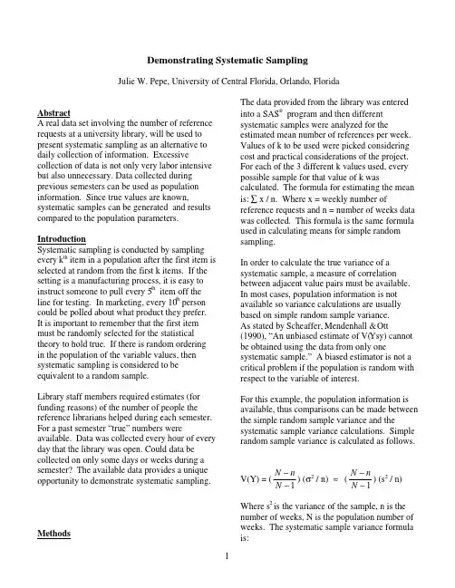
Demonstrating Systematic SamplingJulie W. Pepe, University of Central Florida, Orlando, FloridaAbstractA real data set involving the number of reference requests at a university library, will be used to present systematic sampling as an alternative to daily collection of information. Excessive collection of data is not only very labor intensive but also unnecessary. Data collected during previous semesters can be used as population information. Since true values are known, systematic samples can be generated and results compared to the population parameters. IntroductionSystematic sampling is conducted by sampling every k th item in a population after the first item is selected at random from the first k items. If the setting is a manufacturing process, it is easy to instruct someone to pull every 5th item off the line for testing. In marketing, every 10th person could be polled about what product they prefer. It is important to remember that the first item must be randomly selected for the statistical theory to hold true. If there is random orderingin the population of the variable values, then systematic sampling is considered to be equivalent to a random sample.Library staff members required estimates (for funding reasons) of the number of people the reference librarians helped during each semester. For a past semester “true” numbers were available. Data was collected every hour of every day that the library was open. Could data be collected on only some days or weeks during a semester? The available data provides a unique opportunity to demonstrate systematic sampling. Methods The data provided from the library was entered into a SAS® program and then different systematic samples were analyzed for the estimated mean number of references per week. Values of k to be used were picked considering cost and practical considerations of the project. For each of the 3 different k values used, every possible sample for that value of k was calculated. The formula for estimating the mean is: ∑ x / n. Where x = weekly number of reference requests and n = number of weeks data was collected. This formula is the same formula used in calculating means for simple random sampling.In order to calculate the true variance of a systematic sample, a measure of correlation between adjacent value pairs must be available. In most cases, population information is not available so variance calculations are usually based on simple random sample variance.As stated by Scheaffer, Mendenhall & O tt (1990), “An unbiased estimate of V(Ysy) cannot be obtained using the data from only one systematic sample.” A biased estimator is not a critical problem if the population is random with respect to the variable of interest.For this example, the population information is available, thus comparisons can be made between the simple random sample variance and the systematic sample variance calculations. Simple random sample variance is calculated as follows. V(Y) = (N nN−−1) (σ2 / n) ≈ (N nN−−1) (s2 / n)Where s2 is the variance of the sample, n is the number of weeks, N is the population number of weeks. The systematic sample variance formula is:V(Ysy) = (σ2 / n)[1+(n-1)ρ]where ρ = ()()k nMST SSTn SST−−−11ρ = intracluster correlationMST = mean square totalSST = sums of squares totalk= value of k pickedn= sample sizeThe values necessary are available from PROC ANOVA or PROC GLM output.ResultsPROC MEANS was used to calculate the means and variances of each systematic sample.Table 1 shows the results of k=4, k=3 and k=2 for samples from the 110 weeks of data available. Simple random sample confidence intervals for the mean were calculated in a data step and plotted in Figure 1. This graph gives the client information on what future sample information would look like. Because complete information was available, the plot shows that all the possible samples captured the true mean value (µ=1493). The true mean value is shown as the horizontal line. The vertical lines are formed by the upper and lower limits with the mean marked as a box. Samples 1 to 4 are for k=4, samples 5 to 7 fork=3 and samples 8 to 9 for k=2. The intervals decrease as n increases (k decreases).PROC GLM is used to produce values for calculating the systematic variance. Table 2 shows the PROC GLM results. Calculation of ρ= (3*28)67161-30127481/30127481(27). The resulting value of ρ is -0.030. The intracluster correlation is close to zero therefore, the interpretation is the population is random. The resulting variance calculation for systematic samples would then be 1798.95 (references squared). Bound on the error is ± 83.13 references per week. Figure 2 shows the confidence intervals for samples based on population information (specifically intracluster correlation). As in Figure 1, samples 1 to 4 are for k=4, 5 to 7 for k=3 and 8 to 9 for k=2. SummaryHaving the population information available, reduced the error, yielding smaller confidence intervals. These confidence intervals would not be available when only sample information is collected. These intervals are presented here for demonstration purposes only. Instead of just assuming population values are random, historical data is used to test the assumption. After calculating the intracluster correlation it was determined weeks had random values for the number of reference requests. Thus, systematic sampling is the perfect tool to use in this situation. It cuts down on the amount of data collection yet is an easy method to utilize in the library setting.ReferencesSAS Institute Inc. (1990), SAS Language: Reference, Version 6, First Edition., CaryNC:SAS Institute Inc.SAS Institute Inc. (1990), SAS/STAT Users Guide Vol. 1 and 2, Version 6, Fourth Edition., Cary NC:SAS Institute Inc.Scheaffer, Richard L., Mendenhall, William and Ott, Lyman. (1996), Elementary Survey Sampling, Fifth Edition. Wadsworth Publishing, Belmont, California.The author may be contacted at:University of Central FloridaDepartment of StatisticsPost Office Box 162370Orlando, Florida 32816-2370or pepe@Table 1: Mean and Standard deviations for systematic samples Population Information N= 110 (number of weeks) Mean=1493.44 requestsAnalysis Variable : VALUE-------------------------------------- K = 4 sample 1 -------------------------------------N Mean Std Dev Minimum Maximum28 1466.25 543.1177913 440.0000000 2282.00-------------------------------------- K = 4 sample 2 ------------------------------------- 28 1452.75 609.8147032 336.0000000 2305.00-------------------------------------- K = 4 sample 3 ------------------------------------- 27 1564.00 481.1602963 280.0000000 2155.00-------------------------------------- K = 4 sample 4 ------------------------------------- 27 1493.26 476.4300411 500.0000000 2135.00-------------------------------------- K = 3 sample 1 ------------------------------------- N Mean Std Dev Minimum Maximum37 1484.86 538.2227524 336.0000000 2207.00-------------------------------------- K = 3 sample 2 ------------------------------------- 37 1475.84 535.8665108 280.0000000 2305.00-------------------------------------- K = 3 sample 3 ------------------------------------- 36 1520.33 516.0603508 344.0000000 2282.00-------------------------------------- K = 2 sample 1 ------------------------------------- N Mean Std Dev Minimum Maximum55 1514.24 511.2640821 280.0000000 2282.00-------------------------------------- K = 2 sample 2 ------------------------------------- 55 1472.64 543.7315979 336.0000000 2305.00Table 2: PROC GLM resultsGeneral Linear Models ProcedureDependent Variable: VALUESum of MeanSource DF Squares Square F Value Pr > F Model 3 201485.36936 67161.78979 0.24 0.8698 Error 106 29925995.68519 282320.71401Corrected Total 109 30127481.05455R-Square C.V. Root MSE VALUE Mean0.006688 35.57826 531.33861 1493.4364 Source DF Type I SS Mean Square F Value Pr > FI 3 201485.36936 67161.78979 0.24 0.8698 Source DF Type III SS Mean Square F Value Pr > FI 3 201485.36936 67161.78979 0.24 0.8698Table 3: Confidence Interval CalculationsSimple Random Sample Formula Systematic FormulaOBS LOWER MEAN UPPER N LSYST USYST1 1292.56 1466.25 1639.94 28 1383.12 1549.382 1257.73 1452.75 1647.77 28 1369.62 1535.883 1406.35 1564.00 1721.65 27 1480.87 1647.134 1337.15 1493.26 1649.36 27 1410.13 1576.395 1343.58 1484.86 1626.15 37 1401.73 1567.996 1335.18 1475.84 1616.50 37 1392.71 1558.977 1382.06 1520.33 1658.60 36 1437.20 1603.468 1418.69 1514.24 1609.78 55 1431.11 1597.379 1371.02 1472.64 1574.25 55 1389.51 1555.77。

israel(1992)提出的计算样本大小的公式英文版The Formula for Calculating Sample Size Proposed by Israel (1992)In statistical research, sample size is a crucial element that determines the validity and reliability of the research findings. Selecting an appropriate sample size is essential to ensure that the results of a study are generalizable and accurate. Among the various methods for calculating sample size, the formula proposed by Israel in 1992 stands out as a widely used and reliable approach.The Israel (1992) formula for calculating sample size is based on several key considerations, including the population size, the desired level of confidence, and the margin of error. The formula takes into account these factors to determine the minimum number of samples required to achieve statistically significant results.The formula can be expressed as follows:n = N / (1 + N * e^2)where:n represents the sample sizeN is the population sizee is the margin of error, expressed as a decimal (e.g., 0.05 for a 5% margin of error)This formula allows researchers to calculate the sample size based on their specific research requirements and constraints. By plugging in the values for the population size and the desired margin of error, the formula provides a scientifically sound estimate of the minimum number of samples needed for the study.It is important to note that while the Israel (1992) formula provides a useful starting point for sample size calculation, it may not be applicable in all scenarios. The formula assumes a simple random sampling without replacement, and it may needto be adjusted for more complex sampling designs or specific research contexts.Nevertheless, the Israel (1992) formula remains a valuable tool for researchers seeking to determine an appropriate sample size for their studies. By carefully considering the relevant factors and using this formula, researchers can ensure that their sample size is adequate to support statistically valid and reliable research findings.中文版以色列（1992）提出的计算样本大小的公式在统计研究中，样本大小是决定研究结果的有效性和可靠性的关键因素。

250 400 300 50 Total 1,000
Cluster sampling
Cluster sampling is to draw out a simple random sample of groups or clusters of elements out of a population. This procedure is useful when
5.1 Procedures of sampling and estimation
Sampling design Drawing sample units out of the population Collecting the sample data Organizing the sample data Making the estimation of the quantitative characteristics of the population
A sample of size 1,000 is to be drawn
Stratum Income Population proportion Stratum size
1 2 3 4
under $15,000 15,000-29,999 30.000-50,000 over $50,000
25% 40% 30% 5%
Simple random sampling In simple random sampling, a sample formulated so that each item or person in the population has the same chance / is equally likely to be chosen.

Tommi Jaakkola, MIT AI Lab
3
Parametric density models
• Probability model = a parameterized family of probability distributions • Example: a simple multivariate Gaussian model p(x|µ, Σ) = 1 (2π)p/2|Σ|1/2 1 exp{ − (x − µ)T Σ−1(x − µ) } 2
n
nj ← ˆ
i=1
p(j|i) = Soft # of examples labeled j ˆ
pj ˆ µj ˆ
nj ˆ ← n 1 ← nj ˆ 1 nj ˆ
n
p(j|i) xi ˆ
i=1 n
ˆ Σj ←
Tommi Jaakkola, MIT AI Lab
p(j|i) (xi − µj )(xi − µj )T ˆ ˆ ˆ
x
Fµ,σ2 (x) =
−∞
p(z|µ, σ 2)dz
−1 u ∼ Uniform(0, 1) ⇒ x = Fµ,σ2 (u) ∼ p(x|µ, σ 2)
Tommi Jaakkola, MIT AI Lab
5
Multi-variate Gaussian samples
• A multivariate sample can be constructed from multiple independent one dimensional Gaussian samples: zi ∼ p(zi|µ = 0, σ 2 = 1), z = [z1, . . . , zd]T x = Σ1/2z + µ In this case x ∼ p(x|µ, Σ).

9.1 | 9.2 | 9.3 | 9.4 | 9.5 | 9.6 | 9.7 | 9.8 | 9.9 | 9.10 | 9.11 | 9.13 | 9.14 | 9.15
Background Information

The fast-food manager in Example 9.2 surveyed 40 customers, each of whom rated a new sandwich on a scale of 1 to 10.
Example 9.12
Sample Size Selection for Estimating Reaction to New Sandwich
Controlling Confidence Interval Length
Objective
To find the sample size of customers required to achieve a sufficiently narrow confisandwich.
– the confidence level
• This effect is clear as the confidence level increases, the length of the confidence interval increases as well.
– the sample size(s)
– the data in the sample
• We have control over the data by using the various random sampling plans to reduce variability. • An area of statistics called experimental design suggests how to perform experiments to obtain the most information from a given amount of sample data.

一口气安装800个R包我们周末班准备工作主要就是希望大家学会安装R包 /3727.html首先配置中国大陆特色镜像如果是在海外网络，通常是不需要选择我们这里的代码里面的清华大学和中科院镜像：options()$reposoptions()$BioC_mirroroptions(BioC_mirror="https:///bioc/")options("repos" = c(CRAN="/CRAN/"))options()$reposoptions()$BioC_mirror然后按需安装指定的R包一般来说，我们做生物信息，下面的包肯定是必不可少。

但是需要一个个包去记录，去慢慢安装：# /packages/release/bioc/html/GEOquery.htmlif (!requireNamespace("BiocManager", quietly = TRUE))install.packages("BiocManager")BiocManager::install("KEGG.db",ask = F,update = F)BiocManager::install(c("GSEABase","GSVA","clusterProfiler" ), ask = F,update = F)BiocManager::install(c("GEOquery","limma","impute" ),ask = F,update = F)BiocManager::install(c("org.Hs.eg.db","hgu133plus2.db" ),as k = F,update = F)实际上，大家即使是没有学习过R包安装，也可以看得懂，变化R包名字，就可以一行行运行代码来安装指定的包了！批量安装R包而且不重复安装呢？当然也是有办法的，我在移植一些shiny应用程序就用到过：list.of.packages <- c("shiny","tidyr",'tidyverse',"clusterProfiler","DT","ashr","enrichplot","plotly")# 这个 list.of.packages 变量可以是读取一个包名字文件，比如文末的800多个包：all_packages = rownames(installed.packages())save(all_packages,file = 'all_packages.Rdata')#checking missing packages from listnew.packages <- list.of.packages[!(list.of.packages %in% inst alled.packages()[,"Package"])]new.packagespackToInst <- setdiff(list.of.packages, installed.packages()) packToInstif(T){lapply(packToInst, function(x){BiocManager::install(x,ask = F,update = F)})}lapply(intersect(packagesReq, installed.packages()),function( x){suppressPackageStartupMessages(library(x,character.only = T))})其实你有没有发现，代码反而是多了呢？嘻嘻，虽然代码多了，但是确实是好用！最近我们做了一些服务器共享，需要在上面安装常见的包给用户，这样避免每个人都重复安装同样的包！其中800多个包，如下所示：1 abind2 acepack3 ade44 ADGofTest5 afex6 affxparser7 affy8 affyio9 AIMS10 airway11 ALL12 amap13 AnnoProbe14 annotate15 AnnotationDbi16 AnnotationFilter17 AnnotationHub18 ape19 aplot20 aroma.light21 arules22 arulesViz23 askpass24 assertthat25 backports26 base27 base6428 base64enc29 base64url30 BayesFactor31 bayestestR32 bbmle33 bdsmatrix34 beachmat35 beanplot36 beeswarm37 benchmarkme38 benchmarkmeData39 BH40 bibtex41 Biobase42 BiocFileCache43 BiocGenerics44 BiocIO45 BiocManager46 BiocNeighbors47 BiocParallel48 BiocSingular49 BiocVersion50 biocViews51 biomaRt52 Biostrings53 biovizBase54 bit55 bit6456 bitops57 blob58 bluster59 boot60 bootstrap61 brew62 bridgesampling63 brio64 Brobdingnag65 broom66 broom.mixed67 broomExtra68 BSgenome69 bslib70 bumphunter71 BWStest72 ca73 cachem74 callr75 car76 carData77 caret78 caTools79 ccdrAlgorithm80 cellranger81 checkmate82 ChIPpeakAnno83 ChIPseeker84 chron85 circlize86 class87 cli88 clipr89 clisymbols90 CLL91 clue92 cluster93 clusterProfiler94 ClusterR95 cmprsk96 coda97 codetools98 coin99 colorspace100 colourpicker101 combinat102 cometExactTest103 commonmark104 compiler105 ComplexHeatmap 106 conquer107 ConsensusClusterPlus 108 contfrac109 copula110 corpcor111 correlation112 corrplot113 cowplot114 cpp11115 crayon116 credentials117 crosstalk118 ctc119 curl120 cutoff121 data.table122 datasets123 datawizard124 DBI125 dbplyr126 dbscan127 DDRTree128 DelayedArray129 DelayedMatrixStats 130 deldir131 dendextend132 densityClust133 DEoptimR134 desc135 DescTools136 DESeq2137 deSolve138 devtools139 dichromat140 diffobj141 digest142 diptest143 discretecdAlgorithm 144 do145 DO.db146 docopt147 doParallel148 doRNG149 DOSE150 dotCall64151 downloader152 dplyr153 dqrng154 DT155 dtplyr156 dynamicTreeCut 157 e1071158 EDASeq159 edgeR160 effectsize161 egg162 ellipse163 ellipsis164 elliptic165 emmeans166 EMT167 enrichplot168 EnsDb.Hsapiens.v75 169 ensembldb170 estimability171 europepmc172 evaluate173 Exact174 exactRankTests175 exomeCopy176 ExperimentHub177 expm178 ez179 factoextra180 FactoMineR181 fansi182 farver183 fastcluster184 fastGHQuad185 fastICA186 fastmap187 fastmatch188 FD189 FDb.InfiniumMethylation.hg19 190 ff191 fgsea192 fields193 filelock194 fit.models195 fitdistrplus196 flashClust197 flexmix198 FNN199 fontawesome200 forcats201 foreach202 foreign203 formatR204 Formula205 fpc206 fs207 furrr208 futile.logger209 futile.options210 future211 future.apply212 gameofthrones 213 gapminder214 gargle215 gbRd216 gclus217 gdata218 genefilter219 genefu220 geneplotter221 generics222 genomation223 GenomeInfoDb 224 GenomeInfoDbData 225 GenomicAlignments 226 GenomicFeatures 227 GenomicRanges 228 geometry229 GEOquery230 gert231 GetoptLong233 ggbeeswarm 234 ggbio235 ggcorrplot 236 ggdendro 237 ggExtra238 ggforce239 ggfortify240 ggfun241 ggnetwork 242 ggplot2243 ggplotify 244 ggpubr245 ggraph246 ggrepel247 ggridges248 ggrisk249 ggsci250 ggsignif251 ggstatsplot 252 ggtext253 ggthemes 254 ggtree255 gh256 git2r257 gitcreds258 gld259 glmnet260 glmSparseNet 261 GlobalOptions263 glue264 gmodels265 gmp266 gnm267 GO.db268 goftest269 googledrive 270 googlesheets4 271 GOplot272 GOSemSim 273 gower274 GPArotation 275 gplots276 graph277 graphics278 graphite279 graphlayouts 280 grDevices 281 grid282 gridBase283 gridExtra284 gridGraphics 285 gridtext286 GSEABase 287 gsl288 gsubfn289 GSVA290 gtable291 gtools292 harrypotter293 hash294 haven295 HDF5Array296 here297 hexbin298 hgu133a.db299 hgu133a2.db300 hgu133plus2.db301 hgu95av2.db302 highr303 Hmisc304 hms305 howmany306 HSMMSingleCell307 htmlTable308 htmltools309 htmlwidgets310 httpuv311 httr312 hugene10sttranscriptcluster.db 313 hwriter314 hypergeo315 iC10316 iC10TrainingData317 ica318 idr319 ids320 igraph321 illuminaHumanv3.db322 illuminaio323 impute324 ini325 inline326 insight327 InteractionSet328 interactiveDisplayBase 329 ipred330 IRanges331 IRdisplay332 IRkernel333 irlba334 isoband335 iterators336 jackstraw337 jcolors338 jmv339 jmvcore340 jomo341 jpeg342 jquerylib343 jsonlite344 KEGGREST345 kernlab346 KernSmooth347 km.ci348 KMsurv349 knitr350 kSamples351 labeling352 labelled353 laeken354 lambda.r355 LaplacesDemon 356 lars357 later358 lattice359 latticeExtra 360 lava361 lavaan362 lazyeval363 leaps364 learnr365 leiden366 lfa367 libcoin368 lifecycle369 limma370 linprog371 listenv372 lme4373 lmerTest374 lmom375 lmtest376 locfdr377 locfit378 logspline379 loo380 loose.rock381 lpSolve382 lsei383 lubridate384 lumi385 made4386 maftools387 magic388 magick389 magrittr390 manipulate391 manipulateWidget 392 mapproj393 maps394 maptools395 markdown396 MASS397 Matching398 MatchIt399 mathjaxr400 matlab401 Matrix402 MatrixGenerics 403 MatrixModels 404 matrixStats405 maxstat406 mbkmeans407 mc2d408 mclust409 mcmc410 MCMCpack411 memoise413 metaBMA414 metafor415 metap416 metaplus417 metapod418 methods419 methylumi420 mets421 mgcv422 mice423 mime424 minfi425 miniUI426 minqa427 miRNAtap428 missMDA429 mitml430 mitools431 mlbench432 mnormt433 ModelMetrics434 modelr435 modeltools436 monocle437 multcomp438 multcompView439 MultiAssayExperiment 440 multtest441 munsell443 mvnfast444 mvnormtest445 mvtnorm446 network447 nleqslv448 nlme449 nloptr450 NMF451 nnet452 nomogramFormula 453 nor1mix454 nortest455 npsurv456 numDeriv457 oligo458 oligoClasses459 oompaBase460 openssl461 openxlsx462 ordinal463 org.Dm.eg.db464 org.Hs.eg.db465 org.Mm.eg.db 466 org.Rn.eg.db467 OrganismDbi468 packrat469 paletteer470 palr471 pals473 pan474 pander475 parallel476 parallelly477 parameters 478 patchwork479 pbapply480 pbdZMQ481 pbivnorm482 pbkrtest483 pcaMethods 484 pcaPP485 pd.hugene.2.0.st 486 pdftools487 pec488 performance 489 permute490 pheatmap491 phylobase492 pillar493 pinfsc50494 pixmap495 pkgbuild496 pkgconfig497 pkgload498 pkgmaker499 plogr500 plotly501 plotrix503 PMCMR504 PMCMRplus 505 png506 polspline507 polyclip508 polynom509 prabclus510 pracma511 praise512 preprocessCore 513 prettyunits 514 princurve515 prismatic516 pROC517 processx518 prodlim519 progress520 progressr521 promises522 ProtGenerics 523 proto524 proxy525 ps526 pspline527 psych528 Publish529 purrr530 purrrlyr531 qap532 qlcMatrix533 qpdf534 quadprog 535 quantmod 536 quantreg537 qvalue538 qvcalc539 R.methodsS3 540 R.oo541 R.utils542 R6543 randomForest 544 ranger545 RANN546 rappdirs547 rat2302.db 548 RBGL549 rbibutils550 rcmdcheck 551 RColorBrewer 552 rcompanion 553 rcorpora554 Rcpp555 RcppAnnoy 556 RcppArmadillo 557 RcppEigen 558 RcppGSL559 RcppHNSW 560 RcppParallel 561 RcppProgress562 RcppZiggurat 563 RCurl564 RCy3565 Rdpack566 reactome.db 567 ReactomePA 568 readr569 readxl570 recipes571 regioneR 572 registry573 relimp574 rematch575 rematch2 576 remotes577 renv578 repr579 reprex580 reshape581 reshape2 582 restfulr583 reticulate 584 rex585 Rfast586 rgl587 rhdf5588 rhdf5filters 589 Rhdf5lib 590 Rhtslib591 rio592 riskRegression 593 rJava594 rjson595 RJSONIO596 rlang597 rmarkdown598 rmeta599 Rmpfr600 rms601 RnBeads602 RnBeads.hg38 603 rncl604 RNeXML605 rngtools606 robust607 robustbase608 RobustRankAggreg 609 ROCit610 ROCR611 rootSolve612 ROTS613 roxygen2614 rpart615 rprojroot616 rrcov617 rsample618 Rsamtools619 RSpectra620 RSQLite621 rstan622 rstantools623 rstatix624 rstudioapi625 rsvd626 RTCGA627 RTCGA.clinical 628 RTCGA.miRNASeq 629 RTCGA.rnaseq 630 rtracklayer631 Rtsne632 RUnit633 rvcheck634 rversions635 rvest636 rWikiPathways 637 S4Vectors638 sandwich639 sass640 ScaledMatrix 641 scales642 scater643 scattermore644 scatterpie645 scatterplot3d 646 scico647 scran648 scrime649 scRNAseq650 sctransform651 scuttle652 segmented653 selectr654 seqinr655 seqPattern656 seriation657 sessioninfo658 set659 Seurat660 SeuratObject661 shadowtext662 shape663 shiny664 shinyjs665 shinythemes666 ShortRead667 siggenes668 SingleCellExperiment 669 sitmo670 sjlabelled671 sjmisc672 sjstats673 skimr674 slam675 slider676 slingshot677 smoother678 sn679 sna680 snow681 softImpute682 SomaticCancerAlterations 683 SomaticSignatures684 sourcetools685 sp686 spam687 sparsebn688 sparsebnUtils689 SparseM690 sparseMatrixStats691 sparsesvd692 spatial693 spatstat.core694 spatstat.data695 spatstat.geom696 spatstat.sparse697 spatstat.utils698 splines699 sqldf700 SQUAREM701 stabledist702 StanHeaders703 statmod704 mon705 stats706 stats4707 statsExpressions708 stringi709 stringr710 SummarizedExperiment 711 SuppDists712 survcomp713 survey714 survival715 survivalROC716 survminer717 survMisc718 sva719 swirl720 sys721 table1722 tableone723 taRifx724 TCGAbiolinks725 TCGAbiolinksGUI.data 726 tcltk727 tensor728 testthat729 TFisher730 TH.data731 tibble732 tidygraph733 tidyr734 tidyselect735 tidytree736 tidyverse737 timeDate738 timereg739 timeROC740 tinytex741 TMB743 tmvnsim744 tools745 TrajectoryUtils746 treeio747 triebeard748 tsne749 TSP750 TTR751 tweenr752 TxDb.Dmelanogaster.UCSC.dm3.ensGene 753 TxDb.Dmelanogaster.UCSC.dm6.ensGene 754 TxDb.Hsapiens.UCSC.hg19.knownGene 755 tximport756 tzdb757 uchardet758 ucminf759 UpSetR760 urltools761 usethis762 utf8763 utils764 uuid765 uwot766 V8767 VariantAnnotation768 vcd769 vcdExtra770 vcfR771 vctrs773 VennDiagram 774 VGAM775 VIM776 vipor777 viridis778 viridisLite 779 visNetwork 780 vroom781 waldo782 warp783 webshot 784 WGCNA 785 whisker786 withr787 wordcloud 788 WRS2789 xfun790 XLConnect 791 XML792 xml2793 xopen794 xtable795 xts796 XVector797 yaml798 yulab.utils 799 zeallot800 zinbwave 801 zip802 zlibbioc 803 zoo。

6
A different type of variation is “What if we have no initial estimate of p ˆ?” In this case, the convention is to assume p ˆ = 0.5.
ˆ(1−p ˆ) The reason is that the standard error formula, p n , is largest when p ˆ = 0.5, so this is a conservative assumption that allows for p ˆ being unknown a priori.
7
Sample size to estimate a population mean The issues are similar if we are designing a survey or an experiment to estimate a population mean. In this case, the formula is s ME = t √ ( ‡) n where • ME is the desired margin of error • t is the t-score that we use to calculate the confidence interval, that depends on both the degrees of freedom and the desired confidence level, • s is the standard deviation, • n is the sample size we want to find.
2
Possible answers might be: 1. “We need a margin of error less than 2.5%”. Typical surveys have margins of error ranging from less than 1% to something of the order of 4% — we can choose any margin of error we like but need to specify it. 2. 95% confidence intervals are typical but not in any way mandatory — we could do 90%, 99% or something else entirely. For this example, we assume 95%. 3. May be guided by past surveys or general knowledge of public opinion. Let’s suppose answer is 30%.

Day 5: Statistical 流程Control - What is Statistical 流程Control - Control chart – the voice of the 流程 - 流程control versus 流程capability - Types of control chart available 和its application - Observing trends for control chart - Out of Control reaction - Introduction to Xbar R Chart - Xbar R Chart example - Assignable 和Chance causes in SPC - Rule of thumb for SPC run test --------------------------------------------------------------Break------------------------------------------------------------ Xbar R Chart exercise (using Dice) - Introduction to Xbar S Chart - Implementing Xbar S Chart - 为什么Xbar S Chart ? - Introduction to Individual Moving Range Chart - Implementing Individual Moving Range Chart - 为什么Xbar S Chart ? --------------------------------------------------------------Lunch------------------------------------------------------------ Choosing the sub-group - Choosing the correct sample size Sampling frequency - Introduction to control charts for attribute data - np Charts, p Charts, c Charts, u Charts --------------------------------------------------------------Break------------------------------------------------------------ Attribute control chart exercise (paper clip) 硬商品买卖在阿里巴巴 软商品交易在阿里巧巧 - Out of control not necessarily is bad - Day 5 wrap up

Raw scores are typically computed as the sum of points over items. They have no inherent meaning without reference to something
Relative to the number of possible points Relative to other examinees Relative to a standard (e.g., a pass-fail point) Understanding how difficult the test is (i.e., how difficult it is to obtain particular scores)
Score transformations change an estimated score to some other scale—e.g., a raw score to a “scaled score”. Standard scores are scaled (or transformed) scores that have been converted from one scale to another scale, where the latter has some arbitrarily set mean and standard deviation. Equating adjusts for differences in the relative difficulty of a particular test form so that examinees are indifferent as to which form of the test they happened to take.

Sample Sizes for Multilevel ModelingCora J.M. Maas, Joop J. HoxAddress (both authors):Department of Methodology and StatisticsFaculty of Social Sciences, Utrecht UniversityP.O.B. 80140NL-3508 TC Utrecht, the NetherlandsTel:/Fax: +31 30 2534594 / +31 30 253 5797Sample Sizes for Multilevel ModelingAbstractThe main problem of studying hierarchical systems, which often occur in social statistics, is the dependence of the observations at the lower levels. Multilevel analyzing programs account for this dependence and in recent years these programs have been widely accepted.A problem in multilevel modeling is the question what constitutes a sufficient sample size for accurate estimation. In multilevel analysis, the restriction is often the higher-level sample size. In this paper, a simulation study is used to determine the influence of different sample sizes at the highest level on the accuracy of the estimates (regression coefficients and variances). In addition, the influence of other factors such as the lowest level sample size and different variance distributions between the levels (different intraclass correlations). The results show, that only a small sample size at level two (meaning a sample of 50 or less) leads to biased estimates of the second-level standard errors at the second level. In all of the other simulated conditions the estimates of both the regression coefficients, the variance components and the standard errors are unbiased and accurate.Key words: Multilevel modeling, Sample size, Cluster sampling.Sample Sizes for Multilevel Modeling1.IntroductionSocial research often involves problems that investigate the relationship between individual and society. The general concept is that individuals interact with the social contexts to which they belong, meaning that individual persons are influenced by the social groups or contexts to which they belong, and that the properties of those groups are in turn influenced by the individuals who make up that group. Generally, the individuals and the social groups are conceptualized as a hierarchical system of individuals and groups, with individuals and groups defined at separate levels of this hierarchical system.Even if the analysis includes only variables at the lowest (individual) level, standardmultivariate models are not appropriate. The hierarchical structure of the data creates problems,because the standard assumption of independent and identically distributed observations (i.i.d.) is generally not valid. Multilevel analysis techniques have been developed for the linear regression model (Bryk & Raudenbush, 1992; Goldstein, 1995), and specialized software is now widely available (Bryk, Raudenbush & Congdon, 1996; Rasbash & Woodhouse, 1995).For example, assume that we have data from J groups, with a different number ofrespondents n j in each group. On the respondent level, we have the outcome variable Y ij . We have one explanatory variable X ij on the respondent level, and one group level explanatory variable Z j . To model these data, we have a separate regression model in each group as follows:01ij j j ij ij Y X e ββ=++.(1)Sample Sizes for Multilevel ModelingThe variation of the regression coefficients βj is modeled by a group level regression model, as follows:000010j j j Z u βγγ=++,(2)and110111j j j Z u βγγ=++.(3)The individual-level residuals e ij are assumed to have a normal distribution with mean zero and variance σe 2. The group-level residuals u 0j and u 1j are assumed to have a multivariate normal distribution with expectation zero, and to be independent from the residual errors e ij . The variance of the residual errors u 0j is specified as σ00, and the variance of the residual errors u 1j is specified as σ11.This model can be written as one single regression model by substituting equations (2) and(3) into equation (1). Substitution and earranging terms gives:0010011110ij ij j ij j j ij j ij Y X Z X Z u X u e γγγγ=++++++(4)The segment [γ00 + γ10 X ij + γ01 Z j + γ11 Z j X ij ] in equation (4) contains all the fixed coefficients; it is the fixed (or deterministic) part of the model. The segment [u 0j + u 1j X ij + e ij ] in equation (4)contains all the random error terms; it is the random (or stochastic) part of the model. The termSample Sizes for Multilevel ModelingZ j X ij is an interaction term that appears in the model because of modeling the varying regression slope β1j of respondent level variable X ij with the group level variable Z j.Multilevel models are needed because grouped data violate the assumption of independence of all observations. The amount of dependence can be expressed as the intraclass correlation ρ. In the multilevel model, the intraclass correlation is estimated by specifying an empty model, as follows:Y ij = γ00 + u0j + e ij.(5)Using this model we can estimate the intraclass correlation ρ by the equationρ = σ00 / (σ00 + σe²).(6)The maximum likelihood estimation methods commonly used in multilevel analysis are asymptotic, which translates to the assumption that the sample size is large. This arouses questions about the accuracy of the various estimation methods with relatively small sample sizes. The question is of interest for survey researchers, because multilevel models may be useful in their own right, e.g., as in their use to model interview or region effects (cf. O’Muircheartaigh & Campanelli, 1999; Pickery & Loosvelt, 1998), but also because multilevel techniques offer one way of dealing with clustered or stratified data (Goldstein & Silver, 1989; Snijders, 2001).A recent simulation study on multilevel structural equation modeling (Hox & Maas, 2001) suggests that the size of the intraclass correlation (ICC) also affects the accuracy of the estimates. Therefore, in our simulation, we have varied not only the sample size at the individualSample Sizes for Multilevel Modelingand the group level, but also the intraclass correlation. In general, what is at issue in multilevel modeling is not so much the intraclass correlation, but the design effect, which indicates how much the standard errors are underestimated (Kish, 1965). In cluster samples, the design effect is approximately equal to 1+(average cluster size-1)*ICC. If the design effect is smaller than two, using single level analysis on multilevel data does not seem to lead to overly misleading results (Muthén & Satorra, 1995). In our simulation setup, we have chosen values for the ICC and group sizes that make the design effect larger than two in all simulated conditions.2.Review of existing researchThere are some simulation studies on this topic, which mostly investigate the accuracy of the fixed and random parameters with small sample sizes at either the individual or the group level. Comparatively less research investigates the accuracy of the standard errors used to test specific model parameters.2.1Accuracy of fixed parameters and their standard errorsThe estimates for the regression coefficients appear generally unbiased, for Ordinary Least Squares (OLS), Generalized Least Squares (GLS), as well as Maximum Likelihood estimation (Van der Leeden & Busing, 1994; Van der Leeden et al., 1997). OLS estimates are less efficient; they have a larger sampling error. Kreft (1996), reanalyzing results from Kim (1990), estimates that OLS estimates are about 90% efficient.Sample Sizes for Multilevel ModelingThe OLS based standard errors are severely biased downwards (Snijders & Bosker, 1999). The asymptotic Wald tests, used in most multilevel software, assume large samples. Simulations by Van der Leeden & Busing (1994) and Van der Leeden et al. (1997) suggest that when assumptions of normality and large samples are not met, the standard errors have a small downward bias. GLS estimates of fixed parameters and their standard errors are somewhat less accurate than ML estimates, but workable. In general, a large number of groups appears more important than a large number of individuals per group.2.2Accuracy of random parameters and their standard errorsEstimates of the residual error at the lowest level are generally very accurate. The group level variance components are sometimes underestimated. Simulation studies by Busing (1993) and Van der Leeden and Busing (1994) show that GLS variance estimates are less accurate than ML estimates. The same simulations also indicate that for accurate group level variance estimates many groups (more than 100) are needed (cf. Afshartous, 1995). In contrast, Browne and Draper (2000) show that with as few as six to twelve groups, Restricted ML (RML) estimation provides good variance estimates, and with as few as 48 groups, Full ML (FML) estimation also produces good variance estimates. We will come back to these apparently contradictory results in our discussion.The simulations by Van der Leeden et al. (1997) show that the standard errors used for the Wald test of the variance components are generally estimated too small, with RML again more accurate than FML. Symmetric confidence intervals around the estimated value also do not perform well. Browne and Draper (2000) report similar results. Typically, with 24-30 groups,Sample Sizes for Multilevel ModelingBrowne and Draper report an operating alpha level of about 9%, and with 48-50 groups about 8%. Again, In general, a large number of groups appears more important than a large number of individuals per group.3.Method3.1The simulation model and procedureWe use a simple two-level model, with one explanatory variable at the individual level and one explanatory variable at the group level, conforming to equation (4), which is repeated here:0010011110ij ij j ij j j ij j ij Y X Z X Z u X u e γγγγ=++++++.(4, repeated)Three conditions are varied in the simulation: (1) Number of Groups (NG: three conditions,NG=30,50,100), (2) Group Size (GS: three conditions, GS=5, 30, 50), and (3) Intraclass Correlation (ICC: three conditions, ICC=0.1, 0.2, 0.3).1The number of groups is chosen so that the highest number should be sufficient given the simulations by Van der Leeden et al. (1997). In practice, 50 groups is a frequently occurring number in organizational and school research, and 30 is the smallest number according to Kreft and De Leeuw (Kreft & De Leeuw, 1998). Similarly, the group sizes are chosen so that thehighest number should be sufficient. A group size of 30 is normal in educational research, and a group size of five is normal in family research and in longitudinal research, where themeasurement occasions form the lowest level. The Intra Class Correlations (ICC’s) span theSample Sizes for Multilevel Modelingcustomary level of intraclass correlation coefficients found in studies where the groups are formed by households (Gulliford, Ukoumunne & Chinn, 1999).There are 3×3×3=27 conditions. For each condition, we generated 1000 simulated data sets, assuming normally distributed residuals. The multilevel regression model, like its single-level counterpart, assumes that the explanatory variables are fixed. Therefore, a set of X and Z values are generated from a standard normal distribution to fulfill the requirements of the simulation condition with the smallest total sample size. In the condition with the larger sample sizes, these values are repeated. This ensures that in all simulated conditions the joint distribution of X and Z are the same. The regression coefficients are specified as follows: 1.00 for the intercept, and 0.3 (a medium effect size, cf. Cohen, 1988) for all regression slopes. The residual variance σe2 at the lowest level is 0.5. The residual variance σ00 follows from the specification of the ICC and σe2, given formula (6). Busing (1993) shows that the effects for the intercept variance σ00 and the slope variance σ11 are similar; hence, we chose to use the value of σ00 also for σ11. To simplify the simulation model, without loss of generality, the covariance between the two u-terms is assumed equal to zero.Two Maximum Likelihood functions are common in multilevel estimation: Full ML (FML) and Restricted ML (RML). We use RML, since this is always at least as good as FML, and sometimes better, especially in estimating variance components (Browne, 1998). The software MLwiN (Rasbash et al., 2000) was used for both simulation and estimation.3.2Variables and analysisSample Sizes for Multilevel ModelingThe percentage relative bias is used to indicate the accuracy of the parameter estimates (factorloadings and residual variances). Let θbe the estimate of the population parameter θ, then the percentage relative bias is given by /θθθ−×e j e j100%. The accuracy of the standard errors is investigated by analyzing the observed coverage of the 95% confidence interval. Since the total sample size for each analysis is 27000 simulated conditions, the power is huge. As a result, at the standard significance level of alpha=0.05, extremely small effects becomesignificant. Therefore, our criterion for significance is an alpha = 0.01 for the main effects of the simulated conditions. The interactions are tested blockwise (2-way, 3-way), with a Bonferroni correction added for separate interaction effects. Even at this stricter level ofsignificance, some of the statistically significant biases correspond to differences in parameter estimates that do not show up before the third decimal place. These small effects are discussed in the text, but not included in the various tables.4. Results4.1Convergence and inadmissible solutionsThe estimation procedure converged in all 27000 simulated data sets. The estimation procedure in MLwiN can and sometimes does lead to negative variance estimates. Such solutions are inadmissible, and common procedure is to constrain such estimates to the boundary value of zero. However, all 27000 simulated data sets produced only admissible solutions.Sample Sizes for Multilevel Modeling 4.2Parameter estimatesThe fixed parameter estimates, the intercept and regression slopes, have a negligible bias. The average bias is smaller than 0.05%. The largest bias was found in the condition with the smallest sample sizes in combination with the highest ICC: there the percentage relative bias was 0.3%. This is of course extremely small. Moreover, there are no statistically significant differences in bias across the simulated conditions.The estimates of the random parameters, the variance components, also have a negligible bias. The average bias is smaller than 0.05%. The largest bias was found in the condition with the smallest sample sizes in combination with the highest ICC: there the percentage relative bias was 0.3%.4.3Standard errorsTo assess the accuracy of the standard errors, for each parameter in each simulated data set the 95% confidence interval was established using the asymptotic standard normal distribution (cf. Goldstein, 1995; Longford, 1993). For each parameter a non-coverage indicator variable was set up which is equal to zero if its true value is in the confidence interval, and equal to one if its true value is outside the confidence interval. The effect of the different simulated conditions on the non-coverage was analyzed using logistic regression on these indicator variables.The non-coverage of both fixed and random effects is significantly affected by the number of groups and by the group size. Non-coverage is not sensitive to the Intraclass correlation. TheSample Sizes for Multilevel Modelingeffect of the number of groups on the non-coverage is presented in Table 1, and the effect of the group size on non-coverage is presented in Table 2.======================Tables 1 and 2 about here======================Table 1 shows that the effect of the number of groups on the standard errors of the fixed regression coefficients is small. With 30 groups, the non-coverage rate is 6.0% for the regression coefficient and 6.4% for the intercept, while the nominal non-coverage rate is 5%. We regard this difference as trivial. The effect of the number of groups on the standard errors of the random variance components is definitely larger. With 30 groups, the non-coverage rate for the second-level intercept variance is 8.9%, and the non-coverage rate for the second-level slope variance is 8.8%. Although the coverage is not grotesquely wrong, the 95% confidence interval is clearly too short. The amount of non-coverage here implies that the standard errors for the second-level variance components are estimated about 15% too small. With 50 groups, the effects are smaller, but still not negligible. The non-coverage rates of 7.4% and 7.2% imply that the standard errors are estimated 9% too small.Table 2 shows that the non-coverage of the lowest level variance is improved when the group size increases. The non-coverage of the second-level variances does not improve when the group size increases.5Summary and discussionSample Sizes for Multilevel ModelingConcluding, the point estimates of both the fixed regression coefficients and the random variance components are all estimated without bias, in all of the simulated conditions. The standard errors of the fixed regression coefficients are also estimated accurately. Only the standard errors of the second-level variances are estimated too small when the number of groups is substantially lower than 100. With 30 groups, the standard errors are estimated about 15% too small, resulting in a non-coverage rate of almost 9%, instead of 5%. With 50 groups, the non-coverage drops to about 7.3%. This is clearly different from the nominal 5%, but in practice acceptable.Our simulation results indicate that Maximum Likelihood estimation for multilevel models leads to unbiased point estimates. The asymptotic standard errors are also accurate, with the exception of the standard errors for second-level variances in the case of a small sample of groups (less than 50). These results differ to some extent from the simulation results reported by Busing (1993) and Van der Leeden and Busing (1994). They conclude that for small sample sizes the standard errors and corresponding statistical tests are badly biased, so that about100 groups are needed for accurate estimation of variance components. According to our simulations about fifty groups appears sufficient. However, they use a different simulation design. Busing (1993) uses much higher intraclass correlations, up to 0.80, which are unlikely to occur in actual data. In addition, the simulated second-level sample sizes are much smaller, starting at a sample of 10 groups with 5 observations each. For these simulated conditions, they report both convergence problems and biased standard statistical tests, especially for the variance components. However, their simulation results are comparable when only those conditions are considered that are similar to the conditions in our simulations and those of Browne and Draper (2000).Sample Sizes for Multilevel ModelingTo investigate the limits of our results, we carried out two additional small simulation studies. First, we increased the population values of the residual variances, which decreases the amount of explained variance in the population model. The results were very close to the results reported above. Second, we carried out a simulation with only ten groups of group size five. This simulation was inspired by the dissimilar results of Busing (1993), and by a statement in Snijders and Bosker (1999, p44) that multilevel modeling becomes attractive when the number of groups is larger than ten. This is a very small second-level sample size, but given our simulation results not impossibly small. In this simulation the fixed regression coefficients and variance components were still estimated without bias, except for the second-level variance components when the ICC was low (0.10): there the bias is 25% upwards. The standard errors are now all estimated too small. The non-coverage rates for the fixed effects in this case range between 5.7% and 9.7%, and for the second-level variances they range between 16.3% and 30.4%. Although the standard errors of the fixed effects are still reasonable, the standard errors of the second-level variances are clearly unacceptable. It would seem that having as few as ten groups is too few. If one is interested only in the fixed regression coefficients, it appears feasible, but we would advise to use bootstrapping or other simulation-based methods to assess the sampling variability.6ReferencesAfshartous, D. (1995). Determination of sample size for multilevel model design. Paper presented at the Annual Meeting of the American Educational Research Association, San Francisco, CA.Sample Sizes for Multilevel ModelingBrowne, W.J. (1998). Applying MCMC methods to multilevel models. Unpublished Ph.D.Thesis, University of Bath, UK.Browne, W.J. & Draper, D. (2000). Implementation and performance issues in the Bayesian and likelihood fitting of multilevel models. Computaional Statistics, 15, 391-420.Bryk, A.S. & Raudenbush, S.W. (1992). Hierarchical linear models. Newbury Park, CA: Sage. Bryk, A.S., Raudenbush, S.W. & Congdon, R.T. (1996). HLM. Hierarchical linear and nonlinear modeling with the HLM/2L and HLM?3L programs. Chicago: ScientificSoftware International.Busing, F. (1993). Distribution characteristics of variance estimates in two-level models.Unpublished manuscript. Leiden: Department of Psychometrics and ResearchMethodology, Leiden University.Cohen, J. (1988). Statistical Power Analysis for the Behavioral Sciences. Mahwah, NJ: Erlbaum.O’Muircheartaigh, C. & Campanelli, P. (1999). A multilevel exploration of the role of interviewers in survey non-response. Journal of the Royal Statistical Society, Series A, 162, 437-446.Goldstein, H. (1995). Multilevel Statistical Models. London: Edward Arnold/New York: Halsted.Goldstein, H. & Silver, R. (1989) Multilevel and Multivariate Models in Survey Analysis. In Analysis of Complex Surveys, eds. C.J. Skinner, D. Holt & T.M. Smith. New York:Wiley.Gulliford, M.C., Ukoumunne, O.C. & Chinn, S. (1999). Components of Variance and Intraclass Correlations for the Design of Community-based Surveys and Intervention Studies.Sample Sizes for Multilevel ModelingAmerican Journal of Epidemiology, 149, 876-883. Longford, N.T. (1993). Randomcoefficient models. Oxford: Clarendon Press.Hox, J.J. & Maas, C.J.M. (2001). The Accuracy of Multilevel Structural Equation Modeling With Pseudobalanced Groups and Small Samples. Structural Equation Modeling, 8, 157-174.Kim K.-S. (1990). Multilevel data analysis: A comparison of analytical alternatives.Unpublished Ph.D. thesis, University of California, Los Angeles.Kish, L. (1965). Survey sampling. New York: Wiley.Kreft, I.G.G. (1996): Are Multilevel Techniques Necessary? An Overview, Including Simulation Studies. Unpublished Report, California State University, Los Angeles.Kreft & De Leeuw (1998). Introducing multilevel modeling. Newbury Park, CA: Sage. Longford, N.T. (1993). Random coefficient models. Oxford: Clarendon Press.Muthén, B. & Satorra, A. (1995). Complex sample data in structural equation modeling. In P.V.Marsden (Ed.), Sociological methodology (pp. 267-316). Oxford, England: Blackwell. O’Muircheartaigh, C. & Campanelli, P. (1999). A multilevel exploration of the role of interviewers in survey non-response. Journal of the Royal Statistical Society, Series A, 162, 437-446.Pickery, J. & Loosveldt, G. (1998). The impact of respondent and interviewer characteristics on the number of ‘no opinion’answers. Quality & Quantity, 32, 31-45.Rasbash, J., Browne, W., Goldstein, H., Yang, M., Plewis, I., Healy, M., Woodhouse, G., Draper, D., Langford, I. & Lewis, T. (2000). A user’s guide to MlwiN. London: Multilevel Models Project, University of London.Sample Sizes for Multilevel ModelingRasbash, J., & Woodhouse, G. (1995). MLn command reference. London: Institute of Education, University of London.Snijders, T.A.B. & Bosker, R.J. (1999). Multilevel analysis. An introduction to basic and advanced multilevel modeling. Sage Publications: London-Thousand Oaks-New Delhi. Snijders, T.A.B. (2001). Sampling. In A. Leyland & H. Goldstein (eds.). Multilevel Modelling of Health Statistics. New York: Wiley.Van der Leeden, R., & Busing, F. (1994). First iteration versus IGLS?RIGLS estimates in two-level models: A Monte Carlo study with ML3. Unpublished manuscript, Department of Psychometrics and Research Methodology, Leiden University.Van der Leeden, R., Busing, F., & Meijer, E. (1997): Applications of Bootstrap Methods for Two-level Models. Unpublished paper, Multilevel Conference, Amsterdam, April 1-2, 1997.Sample Sizes for Multilevel ModelingTable 1.Influence of the Number of Groups on the non-coverage of the 95% confidence interval_____________________________________________________________________ Parameter Number of Groups_____________________________________________________________________3050100p-value_______________________________________________________U00.0890.0740.060.0000U10.0880.0720.057.0000E00.0580.0560.049.0102INT0.0640.0570.053.0057X0.0600.0570.050.0058_____________________________________________________________________Sample Sizes for Multilevel ModelingTable 2Influence of the Group Size on the non-coverage of the 95% confidence interval _____________________________________________________________________ Parameter Group Size53050p-value__________________________________________________U00.0740.0750.074.9419U10.0780.0660.072.0080E00.0610.0510.051.0055_____________________________________________________________________Sample Sizes for Multilevel Modeling Footnote:1 Corrections for clustering based on the design effect (Kish, 1965) assume equal group sizes; multilevel analysis does not. We carried out some preliminary simulations to assess if having balanced or unbalanced groups has any influence on multilevel ML estimates. There was no effect of balance on the multilevel estimates or their standard errors.。

0.35
0.3
H0
0.25 0.2
Hβ
0.15
0.1
0.05
0
-4
-3
-2
-1
0
1
2
3
4
5
6
Power of the test
0.5
0.45
0.4
0.35
0.3
H0
0.25 0.2
Hβ
0.15
0.1
0.05
0
-4
-3
-2
-1
0
1
2
3
4
5
6
Power: main ingredients
1. Effect Size 2. Sample Size 3. Variance 4. Clustering 5. Non-Compliance
160 140 120 100
80 60 40 20
0
0 5 10 15 20 25 30 35 40 45 50 55 60 65 70 75 80 85 90 95 100
test scores
control treatment
Two key statistical principles
1. THE LAW OF LARGE NUMBERS The more observations you have, the closer most averages are to the true average
0.5
0.45
0.4
0.35
0.3
0.25
0.2
0.15
0.1
0.05
0
-4
-3
-2

THE UNIVERSITY OF WESTERN ONTARIOLONDON CANADAECONOMICS 2222A - 001TOPIC 7 Tutorial ExercisesJ. Knight Fall 2010Office:4029 SSCPhone:519 661-3489Q.1We are concerned with the sampling scheme of drawing without replacement (orderdisregarded) a simple random sample of size n = 2 from the following population of size N = 5.X :3,5,7,9,11(a)How many samples of size 2 are possible?(b)Construct a probability distribution table for the sample mean and graph it.(c)Verify thatE X ()=μand Var(X )n N n N =−−⎛⎝⎜⎞⎠σ21Q.2Repeat Q.1 using sampling with replacement and show for part (c)E X ()=μand Var X n()=σ2Q.3Suppose we are to take a simple random sample of size n = 50 from an infinite populationhaving mean = 117 and variance 200. Assume the variable of interest is continuous, but that we do not know the distribution of X . Find:(a)Pr .(.)X <1202(b)Pr (115.4 < < 116.8).X (c)The value of above which approximately 91.31% of all sample means chosen inX the above manner will be.2Q.4 A manufacturer has ordered a shipment of 3,000 boxes of small parts. When the shipment arrives, a simple random sample of 25 boxes will be taken and the number of parts in each box counted. If the average number of parts per box is less than 98, the shipment will be rejected. The distribution of the number of parts per box is unknown, but past experience indicates that the mean is 100 and variance 50.What is the probability that the shipment will be accepted?Q.5 A company that manufactures ball-point pens knows from past experience that its percentage defective is 12%. What is the probability of selecting a simple random sample of size 144 with a sample proportion defective of over 14% when sampling from a lot of size N = 2000? Use the continuity correction.。