《数据结构与算法》课后习题答案
- 格式:doc
- 大小:736.00 KB
- 文档页数:37

第1章绪论习题1.简述下列概念:数据、数据元素、数据项、数据对象、数据结构、逻辑结构、存储结构、抽象数据类型。
2.试举一个数据结构的例子,叙述其逻辑结构和存储结构两方面的含义和相互关系。
3.简述逻辑结构的四种基本关系并画出它们的关系图。
4.存储结构由哪两种基本的存储方法实现?5.选择题(1)在数据结构中,从逻辑上可以把数据结构分成()。
A.动态结构和静态结构 B.紧凑结构和非紧凑结构C.线性结构和非线性结构 D.内部结构和外部结构(2)与数据元素本身的形式、内容、相对位置、个数无关的是数据的()。
A.存储结构 B.存储实现C.逻辑结构 D.运算实现(3)通常要求同一逻辑结构中的所有数据元素具有相同的特性,这意味着()。
A.数据具有同一特点B.不仅数据元素所包含的数据项的个数要相同,而且对应数据项的类型要一致C.每个数据元素都一样D.数据元素所包含的数据项的个数要相等(4)以下说法正确的是()。
A.数据元素是数据的最小单位B.数据项是数据的基本单位C.数据结构是带有结构的各数据项的集合D.一些表面上很不相同的数据可以有相同的逻辑结构(5)以下与数据的存储结构无关的术语是()。
A.顺序队列 B. 链表 C.有序表 D. 链栈(6)以下数据结构中,()是非线性数据结构A.树 B.字符串 C.队 D.栈6.试分析下面各程序段的时间复杂度。
(1)x=90; y=100;while(y>0)if(x>100){x=x-10;y--;}else x++;(2)for (i=0; i<n; i++)for (j=0; j<m; j++)a[i][j]=0;(3)s=0;for i=0; i<n; i++)for(j=0; j<n; j++)s+=B[i][j];sum=s;(4)i=1;while(i<=n)i=i*3;(5)x=0;for(i=1; i<n; i++)for (j=1; j<=n-i; j++)x++;(6)x=n; //n>1y=0;while(x≥(y+1)* (y+1))y++;(1)O(1)(2)O(m*n)(3)O(n2)(4)O(log3n)(5)因为x++共执行了n-1+n-2+……+1= n(n-1)/2,所以执行时间为O(n2)(6)O()第2章线性表1.选择题(1)一个向量第一个元素的存储地址是100,每个元素的长度为2,则第5个元素的地址是()。

大学《数据结构与算法分析》课程习题及参考答案模拟试卷一一、单选题(每题 2 分,共20分)1.以下数据结构中哪一个是线性结构?( )A. 有向图B. 队列C. 线索二叉树D. B树2.在一个单链表HL中,若要在当前由指针p指向的结点后面插入一个由q指向的结点,则执行如下( )语句序列。
A. p=q; p->next=q;B. p->next=q; q->next=p;C. p->next=q->next; p=q;D. q->next=p->next; p->next=q;3.以下哪一个不是队列的基本运算?()A. 在队列第i个元素之后插入一个元素B. 从队头删除一个元素C. 判断一个队列是否为空D.读取队头元素的值4.字符A、B、C依次进入一个栈,按出栈的先后顺序组成不同的字符串,至多可以组成( )个不同的字符串?A.14B.5C.6D.85.由权值分别为3,8,6,2的叶子生成一棵哈夫曼树,它的带权路径长度为( )。
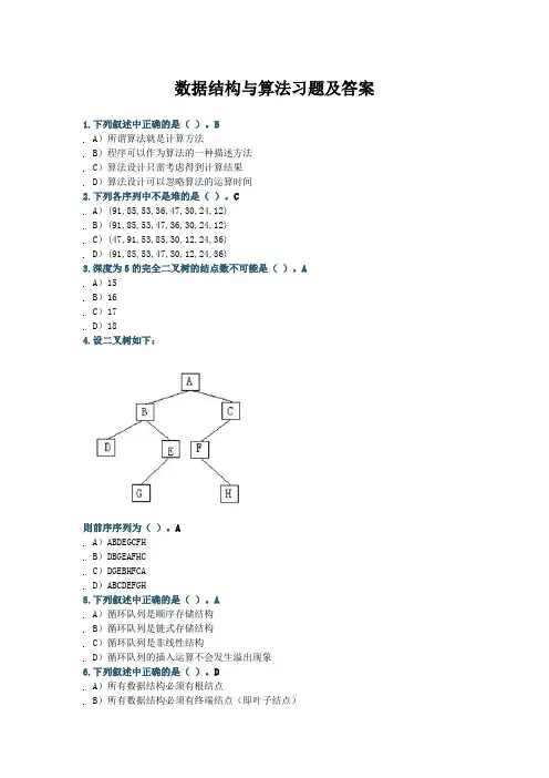
以下6-8题基于图1。
6.该二叉树结点的前序遍历的序列为( )。
A.E、G、F、A、C、D、BB.E、A、G、C、F、B、DC.E、A、C、B、D、G、FD.E、G、A、C、D、F、B7.该二叉树结点的中序遍历的序列为( )。
A. A、B、C、D、E、G、FB. E、A、G、C、F、B、DC. E、A、C、B、D、G、FE.B、D、C、A、F、G、E8.该二叉树的按层遍历的序列为( )。
A.E、G、F、A、C、D、B B. E、A、C、B、D、G、FC. E、A、G、C、F、B、DD. E、G、A、C、D、F、B9.下面关于图的存储的叙述中正确的是( )。
A.用邻接表法存储图,占用的存储空间大小只与图中边数有关,而与结点个数无关B.用邻接表法存储图,占用的存储空间大小与图中边数和结点个数都有关C. 用邻接矩阵法存储图,占用的存储空间大小与图中结点个数和边数都有关D.用邻接矩阵法存储图,占用的存储空间大小只与图中边数有关,而与结点个数无关10.设有关键码序列(q,g,m,z,a,n,p,x,h),下面哪一个序列是从上述序列出发建堆的结果?( )A. a,g,h,m,n,p,q,x,zB. a,g,m,h,q,n,p,x,zC. g,m,q,a,n,p,x,h,zD. h,g,m,p,a,n,q,x,z二、填空题(每空1分,共26分)1.数据的物理结构被分为_________、________、__________和___________四种。
Chapter11:Amortized Analysis11.1When the number of trees after the insertions is more than the number before.11.2Although each insertion takes roughly log N ,and each DeleteMin takes2log N actualtime,our accounting system is charging these particular operations as2for the insertion and3log N −2for the DeleteMin. The total time is still the same;this is an accounting gimmick.If the number of insertions and DeleteMins are roughly equivalent,then it really is just a gimmick and not very meaningful;the bound has more significance if,for instance,there are N insertions and O (N / log N )DeleteMins (in which case,the total time is linear).11.3Insert the sequence N ,N +1,N −1,N +2,N −2,N +3,...,1,2N into an initiallyempty skew heap.The right path has N nodes,so any operation could takeΩ(N )time. 11.5We implement DecreaseKey(X,H)as follows:If lowering the value of X creates a heaporder violation,then cut X from its parent,which creates a new skew heap H 1with the new value of X as a root,and also makes the old skew heap H smaller.This operation might also increase the potential of H ,but only by at most log N .We now merge H andH 1.The total amortized time of the Merge is O (log N ),so the total time of theDecreaseKey operation is O (log N ).11.8For the zig −zig case,the actual cost is2,and the potential change isR f ( X )+ R f ( P )+ R f ( G )− R i ( X )− R i ( P )− R i ( G ).This gives an amortized time bound ofAT zig −zig =2+ R f ( X )+ R f ( P )+ R f ( G )− R i ( X )− R i ( P )− R i ( G )Since R f ( X )= R i ( G ),this reduces to=2+ R f ( P )+ R f ( G )− R i ( X )− R i ( P )Also,R f ( X )> R f ( P )and R i ( X )< R i ( P ),soAT zig −zig <2+ R f ( X )+ R f ( G )−2R i ( X )Since S i ( X )+ S f ( G )< S f ( X ),it follows that R i ( X )+ R f ( G )<2R f ( X )−2.ThusAT zig −zig <3R f ( X )−3R i ( X )11.9(a)Choose W (i )=1/ N for each item.Then for any access of node X ,R f ( X )=0,andR i ( X )≥−log N ,so the amortized access for each item is at most3log N +1,and the net potential drop over the sequence is at most N log N ,giving a bound of O (M log N + M + N log N ),as claimed.(b)Assign a weight of q i /M to items i .Then R f ( X )=0,R i ( X )≥log(q i /M ),so theamortized cost of accessing item i is at most3log(M /q i )+1,and the theorem follows immediately.11.10(a)To merge two splay trees T 1and T 2,we access each node in the smaller tree andinsert it into the larger tree.Each time a node is accessed,it joins a tree that is at leasttwice as large;thus a node can be inserted log N times.This tells us that in any sequence of N −1merges,there are at most N log N inserts,giving a time bound of O (N log2N ).This presumes that we keep track of the tree sizes.Philosophically,this is ugly since it defeats the purpose of self-adjustment.(b)Port and Moffet[6]suggest the following algorithm:If T 2is the smaller tree,insert itsroot into T 1.Then recursively merge the left subtrees of T 1and T 2,and recursively merge their right subtrees.This algorithm is not analyzed;a variant in which the median of T 2is splayed to the rootfirst is with a claim of O (N log N )for the sequence of merges.11.11The potential function is c times the number of insertions since the last rehashing step,where c is a constant.For an insertion that doesn’t require rehashing,the actual time is 1,and the potential increases by c ,for a cost of1+ c .If an insertion causes a table to be rehashed from size S to2S ,then the actual cost is 1+ dS ,where dS represents the cost of initializing the new table and copying the old table back.A table that is rehashed when it reaches size S was last rehashed at size S / 2, so S / 2insertions had taken place prior to the rehash,and the initial potential was cS / 2.The new potential is0,so the potential change is−cS / 2,giving an amortized bound of(d − c / 2)S +1.We choose c =2d ,and obtain an O (1)amortized bound in both cases.11.12We show that the amortized number of node splits is1per insertion.The potential func-tion is the number of three-child nodes in T .If the actual number of nodes splits for an insertion is s ,then the change in the potential function is at most1− s ,because each split converts a three-child node to two two-child nodes,but the parent of the last node split gains a third child(unless it is the root).Thus an insertion costs1node split,amor-tized.An N node tree has N units of potential that might be converted to actual time,so the total cost is O (M + N ).(If we start from an initially empty tree,then the bound is O (M ).)11.13(a)This problem is similar to Exercise3.22.Thefirst four operations are easy to imple-ment by placing two stacks,S L and S R ,next to each other(with bottoms touching).We can implement thefifth operation by using two more stacks,M L and M R (which hold minimums).If both S L and S R never empty,then the operations can be implemented as follows:Push(X,D):push X onto S L ;if X is smaller than or equal to the top of M L ,push X onto M L as well.Inject(X,D):same operation as Push ,except use S R and M R .Pop(D):pop S L ;if the popped item is equal to the top of M L ,then pop M L as well.Eject(D):same operation as Pop ,except use S R and M R .FindMin(D):return the minimum of the top of M L and M R .These operations don’t work if either S L or S R is empty.If a Pop or E j ect is attempted on an empty stack,then we clear M L and M R .We then redistribute the elements so that half are in S L and the rest in S R ,and adjust M L and M R to reflect what the state would be.We can then perform the Pop or E j ect in the normal fashion.Fig. 11.1shows a transfor-mation.Define the potential function to be the absolute value of the number of elements in S L minus the number of elements in S R .Any operation that doesn’t empty S L or S R can3,1,4,6,5,9,2,61,2,63,1,4,65,9,2,6 1,4,65,2S L S R M L RL S RM L M R Fig.11.1.increase the potential by only1;since the actual time for these operations is constant,so is the amortized time.To complete the proof,we show that the cost of a reorganization is O (1)amortized time. Without loss of generality,if S R is empty,then the actual cost of the reorganization is | S L | units.The potential before the reorganization is | S L | ;afterward,it is at most1. Thus the potential change is1− | S L | ,and the amortized bound follows.。
数据结构与算法设计课后习题及答案详解1. 习题一:数组求和题目描述:给定一个整数数组,编写一个函数来计算它的所有元素之和。
解题思路:遍历数组,将每个元素累加到一个变量中,最后返回累加和。
代码实现:```pythondef sum_array(arr):result = 0for num in arr:result += numreturn result```2. 习题二:链表反转题目描述:给定一个单链表,反转它的节点顺序。
解题思路:采用三指针法,依次将当前节点的下一个节点指向上一个节点,然后更新三个指针的位置,直到链表反转完毕。
代码实现:```pythonclass ListNode:def __init__(self, val=0, next=None):self.val = valself.next = nextdef reverse_list(head):prev = Nonecurr = headwhile curr:next_node = curr.nextcurr.next = prevprev = currcurr = next_nodereturn prev```3. 习题三:二叉树的层序遍历题目描述:给定一个二叉树,返回其节点值的层序遍历结果。
解题思路:采用队列来实现层序遍历,先将根节点入队,然后循环出队并访问出队节点的值,同时将出队节点的左右子节点入队。
代码实现:```pythonclass TreeNode:def __init__(self, val=0, left=None, right=None): self.val = valself.left = leftself.right = rightdef level_order(root):if not root:return []result = []queue = [root]while queue:level = []for _ in range(len(queue)):node = queue.pop(0)level.append(node.val)if node.left:queue.append(node.left)queue.append(node.right)result.append(level)return result```4. 习题四:堆排序题目描述:给定一个无序数组,使用堆排序算法对其进行排序。
第8 章排序技术课后习题讲解1. 填空题⑴排序的主要目的是为了以后对已排序的数据元素进行()。
【解答】查找【分析】对已排序的记录序列进行查找通常能提高查找效率。
⑵对n个元素进行起泡排序,在()情况下比较的次数最少,其比较次数为()。
在()情况下比较次数最多,其比较次数为()。
【解答】正序,n-1,反序,n(n-1)/2⑶对一组记录(54, 38, 96, 23, 15, 72, 60, 45, 83)进行直接插入排序,当把第7个记录60插入到有序表时,为寻找插入位置需比较()次。
【解答】3【分析】当把第7个记录60插入到有序表时,该有序表中有2个记录大于60。
⑷对一组记录(54, 38, 96, 23, 15, 72, 60, 45, 83)进行快速排序,在递归调用中使用的栈所能达到的最大深度为()。
【解答】3⑸对n个待排序记录序列进行快速排序,所需要的最好时间是(),最坏时间是()。
【解答】O(nlog2n),O(n2)⑹利用简单选择排序对n个记录进行排序,最坏情况下,记录交换的次数为()。
【解答】n-1⑺如果要将序列(50,16,23,68,94,70,73)建成堆,只需把16与()交换。
【解答】50⑻对于键值序列(12,13,11,18,60,15,7,18,25,100),用筛选法建堆,必须从键值为()的结点开始。
【解答】60【分析】60是该键值序列对应的完全二叉树中最后一个分支结点。
2. 选择题⑴下述排序方法中,比较次数与待排序记录的初始状态无关的是()。
A插入排序和快速排序B归并排序和快速排序C选择排序和归并排序D插入排序和归并排序【解答】C【分析】选择排序在最好、最坏、平均情况下的时间性能均为O(n2),归并排序在最好、最坏、平均情况下的时间性能均为O(nlog2n)。
⑵下列序列中,()是执行第一趟快速排序的结果。
A [da,ax,eb,de,bb] ff [ha,gc]B [cd,eb,ax,da] ff [ha,gc,bb]C [gc,ax,eb,cd,bb] ff [da,ha]D [ax,bb,cd,da] ff [eb,gc,ha]【解答】A【分析】此题需要按字典序比较,前半区间中的所有元素都应小于ff,后半区间中的所有元素都应大于ff。
精心整理第1章绪论习题1.简述下列概念:数据、数据元素、数据项、数据对象、数据结构、逻辑结构、存储结构、抽象数据类型。
2.试举一个数据结构的例子,叙述其逻辑结构和存储结构两方面的含义和相互关系。
3.简述逻辑结构的四种基本关系并画出它们的关系图。
4.存储结构由哪两种基本的存储方法实现5A6{x=x-10;y--;}elsex++;(2)for(i=0;i<n;i++)for(j=0;j<m;j++)a[i][j]=0;(3)s=0;fori=0;i<n;i++)for(j=0;j<n;j++)s+=B[i][j];sum=s;(4)i=1;while(i<=n)i=i*3;(5)x=0;for(i=1;i<n;i++)for(j=1;j<=n-i;j++)x++;(6)x=n;n108 C63.5 C1 C-1 C1 Cext=s;(*s).next=(*p).next;C.s->next=p->next;p->next=s->next;D.s->next=p->next;p->next=s;2,=(rear+1)%=(rear+1)%(m+1)(13)最大容量为n的循环队列,队尾指针是rear,队头是front,则队空的条件是()。
A.(rear+1)%n====frontC.rear+1==frontD.(rear-l)%n==front(14)栈和队列的共同点是()。
A.都是先进先出B.都是先进后出C.只允许在端点处插入和删除元素D.没有共同点(15)一个递归算法必须包括()。
A.递归部分B.终止条件和递归部分C.迭代部分D.终止条件和迭代部分(2)回文是指正读反读均相同的字符序列,如“abba”和“abdba”均是回文,但“good”不是回文。
试写一个算法判定给定的字符向量是否为回文。
(提示:将一半字符入栈)根据提示,算法可设计为:0’9’0’9’0’0’9’0’0’9’0’0’0’M-1]实现循环队列,其中M是队列长度。
第1章绪论习题1.简述下列概念:数据、数据元素、数据项、数据对象、数据结构、逻辑结构、存储结构、抽象数据类型。
2.试举一个数据结构的例子,叙述其逻辑结构和存储结构两方面的含义和相互关系。
3.简述逻辑结构的四种基本关系并画出它们的关系图。
4.存储结构由哪两种基本的存储方法实现?5.选择题(1)在数据结构中,从逻辑上可以把数据结构分成()。
A.动态结构和静态结构B.紧凑结构和非紧凑结构C.线性结构和非线性结构D.内部结构和外部结构(2)与数据元素本身的形式、内容、相对位置、个数无关的是数据的()。
A.存储结构B.存储实现C.逻辑结构D.运算实现(3)通常要求同一逻辑结构中的所有数据元素具有相同的特性,这意味着()。
A.数据具有同一特点B.不仅数据元素所包含的数据项的个数要相同,而且对应数据项的类型要一致C.每个数据元素都一样D.数据元素所包含的数据项的个数要相等(4)以下说法正确的是()。
A.数据元素是数据的最小单位B.数据项是数据的基本单位C.数据结构是带有结构的各数据项的集合D.一些表面上很不相同的数据可以有相同的逻辑结构(5)以下与数据的存储结构无关的术语是()。
A.顺序队列 B. 链表 C.有序表 D. 链栈(6)以下数据结构中,()是非线性数据结构A.树B.字符串C.队D.栈6.试分析下面各程序段的时间复杂度。
(1)x=90; y=100;while(y>0)if(x>100){x=x-10;y--;}else x++;(2)for (i=0; i<n; i++)for (j=0; j<m; j++)a[i][j]=0;(3)s=0;for i=0; i<n; i++)for(j=0; j<n; j++)s+=B[i][j];sum=s;(4)i=1;while(i<=n)i=i*3;(5)x=0;for(i=1; i<n; i++)for (j=1; j<=n-i; j++)x++;(6)x=n; //n>1y=0;while(x≥(y+1)* (y+1))y++;(1)O(1)(2)O(m*n)(3)O(n2)(4)O(log3n)(5)因为x++共执行了n-1+n-2+……+1= n(n-1)/2,所以执行时间为O(n2)(6)O(n)第2章线性表1.选择题(1)一个向量第一个元素的存储地址是100,每个元素的长度为2,则第5个元素的地址是()。
数据结构与算法习题及答案1.下列叙述中正确的是()。
BA)所谓算法就是计算方法B)程序可以作为算法的一种描述方法C)算法设计只需考虑得到计算结果D)算法设计可以忽略算法的运算时间3.深度为5的完全二叉树的结点数不可能是()。
AA)15B)16C)17D)184.设二叉树如下:则前序序列为()。
AA)ABDEGCFH5.下列叙述中正确的是()。
AA)循环队列是顺序存储结构B)循环队列是链式存储结构C)循环队列是非线性结构D)循环队列的插入运算不会发生溢出现象7.下列关于算法的描述中错误的是()。
DA)算法强调动态的执行过程,不同于静态的计算公式B)算法必须能在有限个步骤之后终止C)算法设计必须考虑算法的复杂度D)算法的优劣取决于运行算法程序的环境8.设二叉树如下:则中序序列为()。
BA)ABDEGCFH9.线性表的链式存储结构与顺序存储结构相比,链式存储结构的优点有()。
B A)节省存储空间B)插入与删除运算效率高C)便于查找D)排序时减少元素的比较次数11.下列叙述中正确的是()。
CA)所谓有序表是指在顺序存储空间内连续存放的元素序列B)有序表只能顺序存储在连续的存储空间内C)有序表可以用链接存储方式存储在不连续的存储空间内D)任何存储方式的有序表均能采用二分法进行查找12.设二叉树如下:则后序序列为()。
CA)ABDEGCFH13.下列叙述中正确的是()。
BA)结点中具有两个指针域的链表一定是二叉链表B)结点中具有两个指针域的链表可以是线性结构,也可以是非线性结构 C)二叉树只能采用链式存储结构D)循环链表是非线性结构15.带链的栈与顺序存储的栈相比,其优点是()。
CA)入栈与退栈操作方便B)可以省略栈底指针C)入栈操作时不会受栈存储空间的限制而发生溢出D)以上都不对17.下列关于算法复杂度叙述正确的是()。
BA)最坏情况下的时间复杂度一定高于平均情况的时间复杂度B)时间复杂度与所用的计算工具无关C)对同一个问题,采用不同的算法,则它们的时间复杂度是相同的D)时间复杂度与采用的算法描述语言有关19.下列叙述中正确的是()。
数据结构与算法_桂林电子科技大学中国大学mooc课后章节答案期末考试题库2023年1.下面哪种数据结构不是线性结构()参考答案:二叉树2.串S=”myself“,其子串的数目是()参考答案:223.设目标串为‘abccdcdccbaa',模式串为'cdcc',则第()次匹配成功。
参考答案:64.串S='aaab',其next数组为()参考答案:-1 0 1 25.KMP算法相对于BF算法的优点是时间效率高参考答案:正确6.串是一种数据对象和操作都特殊的线性表参考答案:正确7.下面哪个()可能是执行一趟快速排序能够得到的序列参考答案:[41,12,34,45,27] 55 [72,63]8.设主串t的长度为n,模式串p的长度为m,则BF算法的时间复杂度为O(n+m)参考答案:错误9.从一个长度为n的顺序表中删除第i个元素(0 ≤ i≤ n-1)时,需向前移动的元素的个数是()参考答案:n-i-110.对线性表进行二分查找时,要求线性表必须()参考答案:以顺序方式存储,且结点按关键字有序排序11.某线性表中最常用的操作是在最后一个元素之后插入一个元素和删除第一个元素,则采用()存储方式最节省运算时间。
参考答案:仅有尾指针的单循环链表12.最小不平衡子树是指离插入结点最近,且包含不平衡因子结点的子树参考答案:正确13.在单链表中,存储每个结点需有两个域,一个是数据域,另一个是指针域,它指向该结点的( )参考答案:直接后继14.从一个具有n个节点的单链表中查找其值等于x结点时,在查找成功的情况下,需平均比较()个结点参考答案:n/215.对以下单循环链表分别执行下列程序段,说明执行结果中,各个结点的数据域分别是()p = tail→link→link; p→info = tail→info;【图片】参考答案:8,3,6,816.对以下单链表执行如下程序段,说明执行结果中,各个结点的数据域分别是()void fun (Linklist H) //H是带有头结点的单链表{ PNode p,q; p=H->link;H->link=NULL; while (p) { q=p; p=p->link; q->link=H->link; H->link=q; }}【图片】参考答案:8,6,4,217.根据教科书中线性表的实现方法,线性表中的元素必须是()参考答案:相同类型18.若线性表中最常用的操作是存取第i个元素及其前驱和后继元素的值,为了节省时间应采用的存储方式()参考答案:顺序表19.若已知一个栈的入栈序列是1,2,3,…,n,其输出序列为p1,p2,p3,…,pn,若p1=n,则pi为()参考答案:n-i+120.循环队列用数组A[0,m-1]存放其元素值,已知其头尾指针分别是front和rear,则当前队列中的元素个数是()参考答案:(rear-front+m)%m21.已知其头尾指针分别是front和rear,判定一个循环队列QU(最多元素为m)为空的条件是()参考答案:QU—>front= =QU—>rear22.一个队列的入列序列是1,2,3,4,则队列的输出序列是()参考答案:1,2,3,423.已知其头尾指针分别是front和rear,判定一个循环队列QU(最多元素为m)为满的条件是()参考答案:QU—>front= =(QU—>rear+1)%m24.在计算机内实现递归算法时所需的辅助数据结构是( )参考答案:栈25.设循环队列的元素存放在一维数组Q[0‥30]中,队列非空时,front指示队头元素的前一个位置,rear指示队尾元素。
第3章栈和队列一、基础知识题3.1有五个数依次进栈:1,2,3,4,5。
在各种出栈的序列中,以3,4先出的序列有哪几个。
(3在4之前出栈)。
【解答】34215 ,34251,345213.2铁路进行列车调度时,常把站台设计成栈式结构,若进站的六辆列车顺序为:1,2,3,4,5,6,那么是否能够得到435612, 325641, 154623和135426的出站序列,如果不能,说明为什么不能;如果能,说明如何得到(即写出"进栈"或"出栈"的序列)。
【解答】输入序列为123456,不能得出435612和154623。
不能得到435612的理由是,输出序列最后两元素是12,前面4个元素(4356)得到后,栈中元素剩12,且2在栈顶,不可能让栈底元素1在栈顶元素2之前出栈。
不能得到154623的理由类似,当栈中元素只剩23,且3在栈顶,2不可能先于3出栈。
得到325641的过程如下:1 2 3顺序入栈,32出栈,得到部分输出序列32;然后45入栈,5出栈,部分输出序列变为325;接着6入栈并退栈,部分输出序列变为3256;最后41退栈,得最终结果325641。
得到135426的过程如下:1入栈并出栈,得到部分输出序列1;然后2和3入栈,3出栈,部分输出序列变为13;接着4和5入栈,5,4和2依次出栈,部分输出序列变为13542;最后6入栈并退栈,得最终结果135426。
3.3若用一个大小为6的数组来实现循环队列,且当前rear和front的值分别为0和3,当从队列中删除一个元素,再加入两个元素后,rear和front的值分别为多少?【解答】2和43.4设栈S和队列Q的初始状态为空,元素e1,e2,e3,e4,e5和e6依次通过栈S,一个元素出栈后即进队列Q,若6个元素出队的序列是e3,e5,e4,e6,e2,e1,则栈S的容量至少应该是多少?【解答】43.5循环队列的优点是什么,如何判断“空”和“满”。
《数据结构》教材课后习题+答案数据结构第一章介绍数据结构是计算机科学中重要的概念,它涉及到组织和存储数据的方法和技术。
数据结构的选择对于算法的效率有着重要的影响。
本教材为读者提供了丰富的课后习题,以帮助读者巩固所学知识并提高解决问题的能力。
下面是一些选定的习题及其答案,供读者参考。
第二章线性表习题一:给定一个顺序表L,编写一个算法,实现将其中元素逆置的功能。
答案一:算法思路:1. 初始化两个指针i和j,分别指向线性表L的首尾两个元素2. 对于L中的每一个元素,通过交换i和j所指向的元素,将元素逆置3. 当i>=j时,停止逆置算法实现:```pythondef reverse_list(L):i, j = 0, len(L)-1while i < j:L[i], L[j] = L[j], L[i]i += 1j -= 1```习题二:给定两个线性表A和B,编写一个算法,将线性表B中的元素按顺序插入到线性表A中。
答案二:算法思路:1. 遍历线性表B中的每一个元素2. 将B中的元素依次插入到A的末尾算法实现:```pythondef merge_lists(A, B):for element in B:A.append(element)```第三章栈和队列习题一:编写一个算法,判断一个表达式中的括号是否匹配。
表达式中的括号包括小括号"()"、中括号"[]"和大括号"{}"。
答案一:算法思路:1. 遍历表达式中的每一个字符2. 当遇到左括号时,将其推入栈中3. 当遇到右括号时,判断栈顶元素是否与其匹配4. 当遇到其他字符时,继续遍历下一个字符5. 最后判断栈是否为空,若为空则表示括号匹配算法实现:```pythondef is_matching(expression):stack = []for char in expression:if char in "([{":stack.append(char)elif char in ")]}":if not stack:return Falseelif (char == ")" and stack[-1] == "(") or (char == "]" and stack[-1] == "[") or (char == "}" and stack[-1] == "{"):stack.pop()else:return Falsereturn not stack```习题二:利用两个栈实现一个队列。
Chapter 2:Algorithm Analysis2.12/N ,37,√ N ,N ,N log log N ,N log N ,N log (N 2),N log 2N ,N 1.5,N 2,N 2log N ,N 3,2N / 2,2N .N log N and N log (N 2)grow at the same rate.2.2(a)True.(b)False.A counterexample is T 1(N ) = 2N ,T 2(N ) = N ,and f (N ) = N .(c)False.A counterexample is T 1(N ) = N 2,T 2(N ) = N ,and f (N ) = N 2.(d)False.The same counterexample as in part (c)applies.2.3We claim that N log N is the slower growing function.To see this,suppose otherwise.Then,N ε/ √ log N would grow slower than log N .Taking logs of both sides,we find that,under this assumption,ε/ √ log N log N grows slower than log log N .But the first expres-sion simplifies to ε√ logN .If L = log N ,then we are claiming that ε√ L grows slower than log L ,or equivalently,that ε2L grows slower than log 2 L .But we know that log 2 L = ο (L ),so the original assumption is false,proving the claim.2.4Clearly,log k 1N = ο(log k 2N )if k 1 < k 2,so we need to worry only about positive integers.The claim is clearly true for k = 0and k = 1.Suppose it is true for k < i .Then,by L’Hospital’s rule,N →∞lim N log i N ______ = N →∞lim i N log i −1N _______The second limit is zero by the inductive hypothesis,proving the claim.2.5Let f (N ) = 1when N is even,and N when N is odd.Likewise,let g (N ) = 1when N is odd,and N when N is even.Then the ratio f (N ) / g (N )oscillates between 0and ∞.2.6For all these programs,the following analysis will agree with a simulation:(I)The running time is O (N ).(II)The running time is O (N 2).(III)The running time is O (N 3).(IV)The running time is O (N 2).(V) j can be as large as i 2,which could be as large as N 2.k can be as large as j ,which is N 2.The running time is thus proportional to N .N 2.N 2,which is O (N 5).(VI)The if statement is executed at most N 3times,by previous arguments,but it is true only O (N 2)times (because it is true exactly i times for each i ).Thus the innermost loop is only executed O (N 2)times.Each time through,it takes O ( j 2) = O (N 2)time,for a total of O (N 4).This is an example where multiplying loop sizes can occasionally give an overesti-mate.2.7(a)It should be clear that all algorithms generate only legal permutations.The first two algorithms have tests to guarantee no duplicates;the third algorithm works by shuffling an array that initially has no duplicates,so none can occur.It is also clear that the first two algorithms are completely random,and that each permutation is equally likely.The third algorithm,due to R.Floyd,is not as obvious;the correctness can be proved by induction.SeeJ.Bentley,"Programming Pearls,"Communications of the ACM 30(1987),754-757.Note that if the second line of algorithm 3is replaced with the statementSwap(A[i],A[RandInt(0,N-1)]);then not all permutations are equally likely.To see this,notice that for N = 3,there are 27equally likely ways of performing the three swaps,depending on the three random integers.Since there are only 6permutations,and 6does not evenly divide27,each permutation cannot possibly be equally represented.(b)For the first algorithm,the time to decide if a random number to be placed in A [i ]has not been used earlier is O (i ).The expected number of random numbers that need to be tried is N / (N − i ).This is obtained as follows:i of the N numbers would be duplicates.Thus the probability of success is (N − i ) / N .Thus the expected number of independent trials is N / (N − i ).The time bound is thusi =0ΣN −1N −i Ni ____ < i =0ΣN −1N −i N 2____ < N 2i =0ΣN −1N −i 1____ < N 2j =1ΣN j 1__ = O (N 2log N )The second algorithm saves a factor of i for each random number,and thus reduces the time bound to O (N log N )on average.The third algorithm is clearly linear.(c,d)The running times should agree with the preceding analysis if the machine has enough memory.If not,the third algorithm will not seem linear because of a drastic increase for large N .(e)The worst-case running time of algorithms I and II cannot be bounded because there is always a finite probability that the program will not terminate by some given time T .The algorithm does,however,terminate with probability 1.The worst-case running time of the third algorithm is linear -its running time does not depend on the sequence of random numbers.2.8Algorithm 1would take about 5days for N = 10,000,14.2years for N = 100,000and 140centuries for N = 1,000,000.Algorithm 2would take about 3hours for N = 100,000and about 2weeks for N = 1,000,000.Algorithm 3would use 1⁄12minutes for N = 1,000,000.These calculations assume a machine with enough memory to hold the array.Algorithm 4solves a problem of size 1,000,000in 3seconds.2.9(a)O (N 2).(b)O (N log N ).2.10(c)The algorithm is linear.2.11Use a variation of binary search to get an O (log N )solution (assuming the array is preread).2.13(a)Test to see if N is an odd number (or 2)and is not divisible by 3,5,7,...,√N .(b)O (√ N ),assuming that all divisions count for one unit of time.(c)B = O (log N ).(d)O (2B / 2).(e)If a 20-bit number can be tested in time T ,then a 40-bit number would require about T 2time.(f)B is the better measure because it more accurately represents the size of the input.2.14The running time is proportional to N times the sum of the reciprocals of the primes lessthan N .This is O (N log log N ).See Knuth,Volume2,page394.2.15Compute X 2,X 4,X 8,X 10,X 20,X 40,X 60,and X 62.2.16Maintain an array PowersOfX that can befilled in a for loop.The array will contain X ,X 2,X 4,up to X 2 log N .The binary representation of N (which can be obtained by testing even or odd and then dividing by2,until all bits are examined)can be used to multiply the appropriate entries of the array.2.17For N =0or N =1,the number of multiplies is zero.If b (N )is the number of ones in thebinary representation of N ,then if N >1,the number of multiplies used islog N + b (N )−12.18(a)A .(b)B .(c)The information given is not sufficient to determine an answer.We have only worst-case bounds.(d)Yes.2.19(a)Recursion is unnecessary if there are two or fewer elements.(b)One way to do this is to note that if thefirst N −1elements have a majority,then the lastelement cannot change this.Otherwise,the last element could be a majority.Thus if N is odd,ignore the last element.Run the algorithm as before.If no majority element emerges, then return the N th element as a candidate.(c)The running time is O (N ),and satisfies T (N )= T (N / 2)+ O (N ).(d)One copy of the original needs to be saved.After this,the B array,and indeed the recur-sion can be avoided by placing each B i in the A array.The difference is that the original recursive strategy implies that O (log N )arrays are used;this guarantees only two copies. 2.20Otherwise,we could perform operations in parallel by cleverly encoding several integersinto one.For instance,if A=001,B=101,C=111,D=100,we could add A and B at the same time as C and D by adding00A00C+00B00D.We could extend this to add N pairs of numbers at once in unit cost.2.22No.If Low =1,High =2,then Mid =1,and the recursive call does not make progress. 2.24No.As in Exercise2.22,no progress is made.。
第五章习题(1)复习题1、试述数据和数据结构的概念及其区别。
数据是对客观事物的符号表示,是信息的载体;数据结构则是指互相之间存在着一种或多种关系的数据元素的集合。
(P113)2、列出算法的五个重要特征并对其进行说明。
算法具有以下五个重要的特征:有穷性:一个算法必须保证执行有限步之后结束。
确切性:算法的每一步骤必须有确切的定义。
输入:一个算法有0个或多个输入,以刻画运算对象的初始情况,所谓0个输入是指算法本身定除了初始条件。
输出:一个算法有一个或多个输出,以反映对输入数据加工后的结果。
没有输出的算法没有实际意义。
可行性:算法原则上能够精确地运行,而且人们用笔和纸做有限次运算后即可完成。
(P115)3、算法的优劣用什么来衡量?试述如何设计出优秀的算法。
时间复杂度空间复杂度(P117)4、线性和非线性结构各包含哪些种类的数据结构?线性结构和非线性结构各有什么特点?线性结构用于描述一对一的相互关系,即结构中元素之间只有最基本的联系,线性结构的特点是逻辑结构简单。
所谓非线性结构是指,在该结构中至少存在一个数据元素,有两个或两个以上的直接前驱(或直接后继)元素。
树型和图型结构就是其中十分重要的非线性结构,可以用来描述客观世界中广泛存在的层次结构和网状结构的关系。
(P118 P122)5、简述树与二叉树的区别;简述树与图的区别。
树用来描述层次结构,是一对多或多对一的关系;二叉树(Binary Tree)是个有限元素的集合,该集合或者为空、或者由一个称为根(root)的元素及两个不相交的、被分别称为左子树和右子树的二叉树组成。
二叉树是有序的,即若将其左、右子树颠倒,就成为另一棵不同的二叉树。
图也称做网,是一种比树形结构更复杂的非线性结构。
在图中,任意两个节点之间都可能相关,即节点之间的邻接关系可以是任意的,图表示的多对多的关系。
(P121-P124)6、请举出遍历算法在实际中使用的例子。
提示:根据实际生活中需要逐个访问处理的情况举例。
第一章绪论习题练习答案1.1 简述下列概念:数据、数据元素、数据类型、数据结构、逻辑结构、存储结构、线性结构、非线性结构。
● 数据:指能够被计算机识别、存储和加工处理的信息载体。
● 数据元素:就是数据的基本单位,在某些情况下,数据元素也称为元素、结点、顶点、记录。
数据元素有时可以由若干数据项组成。
● 数据类型:是一个值的集合以及在这些值上定义的一组操作的总称。
通常数据类型可以看作是程序设计语言中已实现的数据结构。
● 数据结构:指的是数据之间的相互关系,即数据的组织形式。
一般包括三个方面的内容:数据的逻辑结构、存储结构和数据的运算。
● 逻辑结构:指数据元素之间的逻辑关系。
● 存储结构:数据元素及其关系在计算机存储器内的表示,称为数据的存储结构.● 线性结构:数据逻辑结构中的一类。
它的特征是若结构为非空集,则该结构有且只有一个开始结点和一个终端结点,并且所有结点都有且只有一个直接前趋和一个直接后继。
线性表就是一个典型的线性结构。
栈、队列、串等都是线性结构。
● 非线性结构:数据逻辑结构中的另一大类,它的逻辑特征是一个结点可能有多个直接前趋和直接后继。
数组、广义表、树和图等数据结构都是非线性结构。
1.2 试举一个数据结构的例子、叙述其逻辑结构、存储结构、运算三个方面的内容。
答:例如有一张学生体检情况登记表,记录了一个班的学生的身高、体重等各项体检信息。
这张登记表中,每个学生的各项体检信息排在一行上。
这个表就是一个数据结构。
每个记录(有姓名,学号,身高和体重等字段)就是一个结点,对于整个表来说,只有一个开始结点(它的前面无记录)和一个终端结点(它的后面无记录),其他的结点则各有一个也只有一个直接前趋和直接后继(它的前面和后面均有且只有一个记录)。
这几个关系就确定了这个表的逻辑结构是线性结构。
这个表中的数据如何存储到计算机里,并且如何表示数据元素之间的关系呢? 即用一片连续的内存单元来存放这些记录(如用数组表示)还是随机存放各结点数据再用指针进行链接呢? 这就是存储结构的问题。
第5章习题解答2- 9, 0-6, 4-9, 2-6, 6-4;(1) 请确定图中各个顶点的度; (2) 给出图的连通分量;(3)列出至少有三个顶点的简单路径。
[解答]由题意得到的图如图5-1所示。
[解答]如图5-2所示,分别为1个顶点,2个顶点,3个顶点,4个顶点,5个顶点和6个顶点 的无向完全图。
5. 1 已知一个图有。
到9 一共10个顶点, 图中边为:3-7,1-4, 7-8, 0-5, 5-2, 3-8,(1)顶点:0 12 3 4 顶点的度:213232⑵连通分量1: 连通分量2: (3)连通分量1:连通分量2中:4-6-0, 4-6-2, 6-2-5, 6-2-9, 9-2-6, 0-5-2,如图5-1 (b)所示。
如图5-1 (a)所示。
3- 7-8; 1-4-6, 1-4-9 4- 9-2, 6-0-5, 6-4一9, 9—2-5,共有13条。
5.2向完全图。
请分别画出1个顶点,2个顶点, 3个顶点,4个顶点,5个顶点和6个顶点的无图5-15.3 若无向图G有15条边,有3个度为4的顶点,其余顶点的度不大于3,图G至少有多少个顶点?[解答]设图G至少有x个顶点,根据握手定理有:3 X4 + 3 (x-3) =2X15, x=9(个)5.4 试证明有/个顶点的任何无环连通图均有V -1条边。
[解答]无环连通图即为树。
根据树的性质,有V个顶点的树均有V-1条边。
5.5对于一个有r个顶点和的无向完全图,请问一共有多少个子图?[解答]V 2一共有个子图。
i=05.6对于一个有V个顶点和E条边的无向图,请给出其连通分量个数的上界和下界。
[解答]根据无向图中顶点和边的关系可知,E必然满足0WEWK(片1)/2,由分析可得到:V-E if E<V-1 c = dmin[1 if E>V-1M=V-(l + Jl + 8E)/2 E<V(V-1)/2提示:在不形成环的情况下,连通分量数目达到最小值;当某个连通分量为完全图时, 连通分量数目达到最大值。
2.3 课后习题解答 2.3.2 判断题 1.线性表的逻辑顺序与存储顺序总是一致的。(×) 2.顺序存储的线性表可以按序号随机存取。(√) 3.顺序表的插入和删除操作不需要付出很大的时间代价,因为每次操作平均只有近一半的元素需要移动。(×) 4.线性表中的元素可以是各种各样的,但同一线性表中的数据元素具有相同的特性,因此属于同一数据对象。(√) 5.在线性表的顺序存储结构中,逻辑上相邻的两个元素在物理位置上并不一定相邻。(×) 6.在线性表的链式存储结构中,逻辑上相邻的元素在物理位置上不一定相邻。(√) 7.线性表的链式存储结构优于顺序存储结构。(×) 8.在线性表的顺序存储结构中,插入和删除时移动元素的个数与该元素的位置有关。(√) 9.线性表的链式存储结构是用一组任意的存储单元来存储线性表中数据元素的。(√) 10.在单链表中,要取得某个元素,只要知道该元素的指针即可,因此,单链表是随机存取的存储结构。(×) 11.静态链表既有顺序存储的优点,又有动态链表的优点。所以它存取表中第i个元素的时间与i无关。(×) 12.线性表的特点是每个元素都有一个前驱和一个后继。(×)
2.3.3 算法设计题 1.设线性表存放在向量A[arrsize]的前elenum个分量中,且递增有序。试写一算法,将x 插入到线性表的适当位置上,以保持线性表的有序性,并且分析算法的时间复杂度。 【提示】直接用题目中所给定的数据结构(顺序存储的思想是用物理上的相邻表示逻辑上的相邻,不一定将向量和表示线性表长度的变量封装成一个结构体),因为是顺序存储,分配的存储空间是固定大小的,所以首先确定是否还有存储空间,若有,则根据原线性表中元素的有序性,来确定插入元素的插入位置,后面的元素为它让出位置,(也可以从高下标端开始一边比较,一边移位)然后插入x ,最后修改表示表长的变量。 int insert (datatype A[],int *elenum,datatype x) /*设elenum为表的最大下标*/ {if (*elenum==arrsize-1) return 0; /*表已满,无法插入*/
else {i=*elenum; while (i>=0 && A[i]>x) /*边找位置边移动*/ {A[i+1]=A[i]; i--; } A[i+1]=x; /*找到的位置是插入位的下一位*/ (*elenum)++; return 1; /*插入成功*/ } } 时间复杂度为O(n)。 2.已知一顺序表A,其元素值非递减有序排列,编写一个算法删除顺序表中多余的值相同的元素。 【提示】对顺序表A,从第一个元素开始,查找其后与之值相同的所有元素,将它们删除;再对第二个元素做同样处理,依此类推。 void delete(Seqlist *A) {i=0; while(ilast) /*将第i个元素以后与其值相同的元素删除
*/ {k=i+1; while(k<=A->last&&A->data[i]==A->data[k]) k++; /*使k指向第一个与A[i]不同的元素*/
n=k-i-1; /*n表示要删除元素的个数*/ for(j=k;j<=A->last;j++) A->data[j-n]=A->data[j]; /*删除多余元素*/ A->last= A->last -n; i++; } } 3.写一个算法,从一个给定的顺序表A中删除值在x~y(x<=y)之间的所有元素,要求以较高的效率来实现。 【提示】对顺序表A,从前向后依次判断当前元素A->data[i]是否介于x和y之间,若是,并不立即删除,而是用n记录删除时应前移元素的位移量;若不是,则将A->data[i]向前移动n位。n用来记录当前已删除元素的个数。 void delete(Seqlist *A,int x,int y) {i=0; n=0; while (ilast) {if (A->data[i]>=x && A->data[i]<=y) n++; /*若A->data[i] 介于x和y之间,n自增*/ else A->data[i-n]=A->data[i]; /*否则向前移动A->data[i]*/
i++; } A->last-=n; } 4.线性表中有n个元素,每个元素是一个字符,现存于向量R[n]中,试写一算法,使R中的字符按字母字符、数字字符和其它字符的顺序排列。要求利用原来的存储空间,元素移动次数最小。 【提示】对线性表进行两次扫描,第一次将所有的字母放在前面,第二次将所有的数字放在字母之后,其它字符之前。 int fch(char c) /*判断c是否字母*/ {if(c>='a'&&c<='z'||c>='A'&&c<='Z') return (1); else return (0); } int fnum(char c) /*判断c是否数字*/ {if(c>='0'&&c<='9') return (1); else return (0); } void process(char R[n]) {low=0; high=n-1; while(low/*将字母放在前面*/
{while(lowwhile(lowif(low{k=R[low]; R[low]=R[high]; R[high]=k; } } low=low+1; high=n-1; while(low {while(lowwhile(lowif(low{k=R[low]; R[low]=R[high]; R[high]=k; } } } 5.线性表用顺序存储,设计一个算法,用尽可能少的辅助存储空间将顺序表中前m个元素和后n个元素进行整体互换。即将线性表: (a1, a2, … , am, b1, b2, … , bn)改变为: (b1, b2, … , bn , a1, a2, … , am)。 【提示】比较m和n的大小,若m后移n次。 void process(Seqlist *L,int m,int n) {if(m<=n) for(i=1;i<=m;i++) {x=L->data[0]; for(k=1;k<=L->last;k++) L->data[k-1]=L->data[k]; L->data[L->last]=x; } else for(i=1;i<=n;i++) {x=L->data[L->last]; for(k=L->last-1;k>=0;k- -) L->data[k+1]=L->data[k]; L->data[0]=x; } } 6.已知带头结点的单链表L中的结点是按整数值递增排列的,试写一算法,将值为x 的结点插入到表L中,使得L仍然递增有序,并且分析算法的时间复杂度。 LinkList insert(LinkList L, int x) {p=L; while(p->next && x>p->next->data) p=p->next; /*寻找插入位置*/
s=(LNode *)malloc(sizeof(LNode)); /*申请结点空间*/ s->data=x; /*填装结点*/ s->next=p->next; p->next=s; /*将结点插入到链表中*/ return(L); } 7.假设有两个已排序(递增)的单链表A和B,编写算法将它们合并成一个链表C而不改变其排序性。 LinkList Combine(LinkList A, LinkList B) {C=A; rc=C; pa=A->next; /*pa指向表A的第一个结点*/ pb=B->next; /*pb指向表B的第一个结点*/
free(B); /*释放B的头结点*/ while (pa && pb) /*将pa、pb所指向结点中,值较小的一个插入到链表C的表尾*/ if(pa->datadata) {rc->next=pa; rc=pa; pa=pa->next; } else {rc->next=pb; rc=pb; pb=pb->next; } if(pa) rc->next=pa; else rc->next=pb; /*将链表A或B中剩余的部分链接到链表C的表尾*/ return(C); } 8.假设长度大于1的循环单链表中,既无头结点也无头指针,p为指向该链表中某一结点的指针,编写算法删除该结点的前驱结点。 【提示】利用循环单链表的特点,通过s指针可循环找到其前驱结点p及p的前驱结点q,然后可删除结点*p。 viod delepre(LNode *s) {LNode *p, *q;