Differentical Resistivity Geophysics 1996 Jan-Feb

第４５卷　第４期２０２３年７月物探化探计算技术ＣＯＭＰＵＴＩＮＧＴＥＣＨＮＩＱＵＥＳＦＯＲＧＥＯＰＨＹＳＩＣＡＬＡＮＤＧＥＯＣＨＥＭＩＣＡＬＥＸＰＬＯＲＡＴＩＯＮＶｏｌ．４５　Ｎｏ．４Ｊｕｌ．２０２３收稿日期：２０２２ ０４ １９基金项目：陕西省教育厅科学研究计划项目（２２ＪＫ０５２６）第一作者：郑建波（１９９０－），女，硕士，讲师，主要从事电磁勘探方法研究，Ｅ ｍａｉｌ：ｚｈｅｎｇｊｉａｎｂｏｂｏ１９９０＠１６３．ｃｏｍ。

文章编号：１００１ １７４９（２０２３）０４ ０４７８ ０６航空瞬变电磁全时域全空域快速成像郑建波，李美艳（西安外事学院工学院，西安　７１００７７）摘　要：航空瞬变电磁法以其快速高效的优势已获得广泛应用，然而航空瞬变电磁采样密集，数据量巨大。

为了实现航空瞬变电磁观测数据的快速解释，开展航空瞬变电磁快速成像算法研究。

利用反函数定理建立成像迭代格式，并在成像过程中考虑发射源高度和观测时间的影响，进而实现航空瞬变电磁全时域全空域快速成像。

这里首先给出了全时域全空域成像理论和实现方法，然后对航空瞬变电磁装置进行了介绍，最后建立了典型采空区模型，利用开发的航空瞬变电磁全时域全空域视电阻率成像方法进行数据成像，成像结果与真实模型基本一致，验证了方法的有效性。

关键词：航空瞬变电磁；全时域；全空域；成像中图分类号：Ｐ６３１．３ 文献标志码：Ａ 犇犗犐：１０．３９６９／ｊ．ｉｓｓｎ．１００１ １７４９．２０２３．０４．０８０　引言航空瞬变电磁法将电磁探测装置搭载在飞机上，通过发射线圈进行大功率发射，激发地下感应涡流，通过观测断电间歇感应涡流产生的二次磁场的空间和时间分布特征，对地下目标进行快速电磁探测。

由于该方法具有快速、高效、受地形影响小等特点，已被广泛应用于矿产勘查、环境地质调查等诸多领域［１－５］。

由于航空瞬变电磁法在探测过程中进行连续采样，获得海量观测数据，因此具有较高的分辨率。

然而，海量数据量也给航空瞬变电磁数据解释带来了巨大困难。

１０００ ０５６９／２０２２／０３８（０２） ０５４４ ５８ＡｃｔａＰｅｔｒｏｌｏｇｉｃａＳｉｎｉｃａ　岩石学报ｄｏｉ：１０ １８６５４／１０００ ０５６９／２０２２ ０２ １６江南造山带深部边界及成矿制约：来自综合地球物理的认识严加永１，２，３　吕庆田１，２　张永谦１，２　刘卫强４　王栩１，２　陈昌昕１，２　徐 １，２　刘家豪１，２ＹＡＮＪｉａＹｏｎｇ１，２，３，Ｌ ＱｉｎｇＴｉａｎ１，２，ＺＨＡＮＧＹｏｎｇＱｉａｎ１，２，ＬＩＵＷｅｉＱｉａｎｇ４，ＷＡＮＧＸｕ１，２，ＣＨＥＮＣｈａｎｇＸｉｎ１，２，ＸＵＹａｏ１，２ａｎｄＬＩＵＪｉａＨａｏ１，２１ 中国地质科学院，北京　１０００３７２ 中国地质调查局中国地质科学院地球深部探测中心，北京　１０００３７３ 东华理工大学地球物理与测控学院，南昌　３３００１３４ 中国石油大学（北京）地球物理学院，北京　１０２２４９１ ＣｈｉｎｅｓｅＡｃａｄｅｍｙｏｆＧｅｏｌｏｇｉｃａｌＳｃｉｅｎｃｅｓ，Ｂｅｉｊｉｎｇ１０００３７，Ｃｈｉｎａ２ ＣｈｉｎａＤｅｅｐＥｘｐｌｏｒａｔｉｏｎＣｅｎｔｅｒ，ＣｈｉｎａＧｅｏｌｏｇｉｃａｌＳｕｒｖｅｙ＆ＣｈｉｎｅｓｅＡｃａｄｅｍｙｏｆＧｅｏｌｏｇｉｃａｌＳｃｉｅｎｃｅｓ，Ｂｅｉｊｉｎｇ１０００３７，Ｃｈｉｎａ３ ＳｃｈｏｏｌｏｆＧｅｏｐｈｙｓｉｃｓａｎｄＭｅａｓｕｒｅｍｅｎｔ ｃｏｎｔｒｏｌＴｅｃｈｎｏｌｏｇｙ，ＥａｓｔＣｈｉｎａＵｎｉｖｅｒｓｉｔｙｏｆＴｅｃｈｎｏｌｏｇｙ，Ｎａｎｃｈａｎｇ３３００１３，Ｃｈｉｎａ４ ＣｏｌｌｅｇｅｏｆＧｅｏｐｈｙｓｉｃｓ，ＣｈｉｎａＵｎｉｖｅｒｓｉｔｙｏｆＰｅｔｒｏｌｅｕｍＢｅｉｊｉｎｇ，Ｂｅｉｊｉｎｇ１０２２４９，Ｃｈｉｎａ２０２１ ０８ ２８收稿，２０２１ １１ ２５改回ＹａｎＪＹ，ＬüＱＴ，ＺｈａｎｇＹＱ，ＬｉｕＷＱ，ＷａｎｇＸ，ＣｈｅｎＣＸ，ＸｕＹａｎｄＬｉｕＪＨ ２０２２ ＴｈｅｄｅｅｐｂｏｕｎｄａｒｉｅｓｏｆＪｉａｎｇｎａｎｏｒｏｇｅｎｉｃｂｅｌｔａｎｄｉｔｓｃｏｎｓｔｒａｉｎｔｓｏｎｍｅｔａｌｌｏｇｅｎｉｃ：Ｆｒｏｍｔｈｅｕｎｄｅｒｓｔａｎｄｉｎｇｏｆｉｎｔｅｇｒａｔｅｄｇｅｏｐｈｙｓｉｃｓ ＡｃｔａＰｅｔｒｏｌｏｇｉｃａＳｉｎｉｃａ，３８（２）：５４４－５５８，ｄｏｉ：１０ １８６５４／１０００ ０５６９／２０２２ ０２ １６Ａｂｓｔｒａｃｔ ＴｈｅＪｉａｎｇｎａｎｏｒｏｇｅｎｉｃｂｅｌｔ，ｌｏｃａｔｅｄｂｅｔｗｅｅｎｔｈｅＹａｎｇｔｚｅａｎｄＣａｔｈａｙｓｉａｎｂｌｏｃｋｓ，ｉｓａｋｅｙｗｉｎｄｏｗｔｏｕｎｄｅｒｓｔａｎｄｔｈｅｅｖｏｌｕｔｉｏｎａｎｄｄｙｎａｍｉｃｐｒｏｃｅｓｓｏｆｔｈｅＳｏｕｔｈＣｈｉｎａＢｌｏｃｋ，ａｎｄｔｏｒｅｖｅａｌｔｈｅｌａｒｇｅ ｓｃａｌｅｍａｇｍａｔｉｓｍａｎｄｔｈｅａｃｃｏｍｐａｎｉｅｄｍｅｔａｌｍｉｎｅｒａｌｒｅｓｏｕｒｃｅｓｉｎｔｈｉｓａｒｅａ Ｐｒｅｄｅｃｅｓｓｏｒｓｈａｖｅｍａｄｅａｌｏｔｏｆｐｒｏｇｒｅｓｓｉｎｉｔｓｔｅｃｔｏｎｉｃｓ，ｐｅｔｒｏｌｏｇｙａｎｄｏｒｅｄｅｐｏｓｉｔｓｃｉｅｎｃｅ，ｂｕｔｔｈｅｒｅａｒｅｌｏｎｇ ｔｅｒｍｄｉｓｐｕｔｅｓｉｎｉｔｓｄｅｆｉｎｉｔｉｏｎ，ｂｏｕｎｄａｒｉｅｓ，ｆｏｒｍａｔｉｏｎａｇｅａｎｄｅｖｏｌｕｔｉｏｎｐｒｏｃｅｓｓ Ｔｈｅｆｕｎｄａｍｅｎｔａｌｒｅａｓｏｎｉｓｔｈａｔｔｈｅｄｅｅｐｓｔｒｕｃｔｕｒｅｉｓｕｎｃｌｅａｒ，ｔｈｅｒｅｆｏｒｅ，ｉｔｉｓｕｒｇｅｎｔｔｏｃａｒｒｙｏｕｔｄｅｅｐｅｘｐｌｏｒａｔｉｏｎｔｏｐｒｏｖｉｄｅｓｕｐｐｏｒｔｆｏｒｄｉｓｐｕｔｅｒｅｓｏｌｕｔｉｏｎ ＴｈｉｓｐａｐｅｒｆｏｃｕｓｅｓｏｎｔｈｅｄｅｅｐｂｏｕｎｄａｒｉｅｓｏｆＪｉａｎｇｎａｎｏｒｏｇｅｎｉｃｂｅｌｔ，ａｎｄｄｅｔｅｃｔｓｔｈｅｄｅｎｓｉｔｙａｎｄｍａｇｎｅｔｉｓｍｂｏｕｎｄａｒｉｅｓａｎｄｉｎｖｅｒｓｅｓｔｈｅｄｅｅｐｅｌｅｃｔｒｉｃａｌｓｔｒｕｃｔｕｒｅｍａｉｎｌｙｂｙｕｓｉｎｇｇｒａｖｉｔｙａｎｄａｅｒｏｍａｇｎｅｔｉｃｄａｔａｔｏｇｅｔｈｅｒｗｉｔｈｓｕｐｐｌｅｍｅｎｔｅｄｍａｇｎｅｔｏｔｅｌｌｕｒｉｃｄａｔａ Ｃｏｍｂｉｎｅｄｗｉｔｈｔｈｅｃｌｕｓｔｅｒａｎａｌｙｓｉｓｒｅｓｕｌｔｓｏｆ７５ｅｌｅｍｅｎｔｓｔｒｅａｍｓｅｄｉｍｅｎｔｇｅｏｃｈｅｍｉｃａｌｄａｔａ，ｉｔｉｓｃｏｎｓｉｄｅｒｅｄｔｈａｔｔｈｅＱｉｎｈａｎｇｊｕｎｃｔｉｏｎｂｅｌｔｉｓｔｈｅｓｏｕｔｈｅａｓｔｂｏｕｎｄａｒｙｏｆｔｈｅＪｉａｎｇｎａｎｏｒｏｇｅｎｉｃｂｅｌｔ，ａｎｄｔｈｅｐｏｓｓｉｂｌｅｄｅｅｐｂｏｕｎｄａｒｙｉｎｔｈｅｎｏｒｔｈｏｆｔｈｅＪｉａｎｇｎａｎｏｒｏｇｅｎｉｃｂｅｌｔｉｓｆｕｒｔｈｅｒｉｎｆｅｒｒｅｄａｎｄｄｅｔｅｒｍｉｎｅｄ Ｏｎｔｈｉｓｂａｓｉｓ，ｔｈｅｆａｕｌｔｓｔｒｕｃｔｕｒｅｓａｒｏｕｎｄｔｈｅＪｉａｎｇｎａｎｏｒｏｇｅｎｉｃｂｅｌｔａｒｅｉｄｅｎｔｉｆｉｅｄａｎｄｒｅ ｄｅｔｅｒｍｉｎｅｄ，ａｎｄｔｈｅｃｏｎｔｒｏｌｏｆｒｅｇｉｏｎａｌｓｔｒｕｃｔｕｒｅｓｏｎｇｏｌｄａｎｄｃｏｐｐｅｒｄｅｐｏｓｉｔｓｉｓａｎａｌｙｚｅｄ ＩｔｉｓｃｏｎｓｉｄｅｒｅｄｔｈａｔｔｈｅｄｅｅｐｂｏｕｎｄａｒｉｅｓａｎｄｄｅｅｐｆａｕｌｔｓｏｆｔｈｅＪｉａｎｇｎａｎｏｒｏｇｅｎｉｃｂｅｌｔｐｌａｙｔｈｅｒｏｌｅｏｆ“ｏｒｅｇｕｉｄｅｐａｔｈ”ｉｎｔｈｅｍｅｔａｌｌｏｇｅｎｉｃｓｙｓｔｅｍ，ａｎｄｐｒｏｖｉｄｅｍｉｎｅｒａｌｓｗｈｉｃｈｄｏｍｉｎａｔｅｄｂｙｍａｎｔｌｅｄｅｒｉｖｅｄｃｏｍｐｏｎｅｎｔｓｓｕｃｈａｓｃｏｐｐｅｒａｎｄｇｏｌｄｆｒｏｍｔｈｅｂｅｇｉｎｎｉｎｇｏｆｔｈｅｆｏｒｍａｔｉｏｎｏｆｄｅｅｐｆａｕｌｔｓ Ｔｈｅｍｉｎｅｒａｌｉｚａｔｉｏｎｉｓｉｎｐｌａｃｅａｔｔｈｅａｐｐｒｏｐｒｉａｔｅｐｏｓｉｔｉｏｎ，ａｎｄｔｈｅｃｏｍｐｌｅｘｔｅｃｔｏｎｉｃｍｏｖｅｍｅｎｔｉｎｔｈｅｌａｔｅｒｓｔａｇｅｒｅａｃｔｉｖａｔｅｓｔｈｅｌｏｃａｌｐｏｓｉｔｉｏｎ，ｅｎｒｉｃｈｅｓａｎｄｍｉｇｒａｔｅｓｔｈｅｏｒｅ ｆｏｒｍｉｎｇｍａｔｅｒｉａｌｓａｇａｉｎ，ａｎｄｆｏｒｍｓｃｏｐｐｅｒｇｏｌｄｄｅｐｏｓｉｔｓｏｆｄｉｆｆｅｒｅｎｔａｇｅｓａｎｄｄｉｆｆｅｒｅｎｔｔｙｐｅｓｉｎｆａｖｏｒａｂｌｅｐｏｓｉｔｉｏｎｓｓｕｃｈａｓｓｅｃｏｎｄａｒｙｆａｕｌｔｓ Ｔｈｅｒｅｆｏｒｅ，ｔｈｅｆａｕｌｔｔｅｃｔｏｎｉｃｉｄｅｎｔｉｆｉｅｄｆｒａｍｅｗｏｒｋｉｎｔｈｉｓｐａｐｅｒｃａｎａｌｓｏｐｒｏｖｉｄｅａｎｉｎｄｉｃａｔｉｏｎｆｏｒｔｈｅｅｘｐｌｏｒａｔｉｏｎｆｏｒｍａｎｔｌｅｃｏｒｒｅｌａｔｅｄｍｅｔａｌｄｅｐｏｓｉｔｓＫｅｙｗｏｒｄｓ Ｊｉａｎｇｎａｎｏｒｏｇｅｎｉｃｂｅｌｔ；Ｇｒａｖｉｔｙａｎｄｍａｇｎｅｔｉｃｄａｔａ；Ｉｎｔｅｇｒａｔｅｄｇｅｏｐｈｙｓｉｃｓ；Ｒｅｓｉｓｔｉｖｉｔｙｉｎｖｅｒｔｅｄｆｒｏｍｍａｇｎｅｔｏｔｅｌｌｕｒｉｃｄａｔａ；Ｇｅｏｃｈｅｍｉｃａｌｃｌｕｓｔｅｒａｎａｌｙｓｉｓ；Ｐａｔｈｗａｙｏｆｍｉｎｅｒａｌｓｙｓｔｅｍ摘　要 江南造山带位于组成华南大陆的扬子地块和华夏地块之间，是揭示华南陆块演化及其动力学过程、探索该地区大规模岩浆多金属成矿作用的关键窗口。

采用电法CT技术探查树木内部结构于仲;张平松;付茂如;程刚【摘要】为探讨直流电法应用于树木内部结构探测的成像效果,通过直流电法层析成像技术对不同种类的树木进行了检测实验研究.运用并行电法进行数据采集,利用弧度修正系数对电性参数进行了修正,获得了较为理想的树干电阻率剖面.三种树木电性剖面对比发现,不同材质的树木电阻率值差异明显,且树干断面电阻率分布整体表现为里高外低的特征.电阻率分布特性可为树木健康状况诊断提供相关技术参数.%With direct current CT technology, the detection experiment among different tree species has been carried out for the sake of studying the imaging results of inner structure of tree trunks. Ideal resistivity distribution profiles have been obtained by the process of data collecting with the Network Parallel Galvanic Exploration System initially and curvature correction for modifying electrical parameters then. By contrast, the conclusion can be drawn that there' s a large variation range among three kind of trees in resistivity. Besides, the internal electrical distribution of tree trunk is that resistivity of the trunk profile is higher inside, and lower outside respectively. Related technical parameters can be provided by resistivity distribution characteristics for diagnosing health symptoms of trees.【期刊名称】《安徽理工大学学报（自然科学版）》【年(卷),期】2012(032)002【总页数】4页(P59-62)【关键词】直流电CT检测技术;电阻率反演;圆柱体结构;弧度修正【作者】于仲;张平松;付茂如;程刚【作者单位】安徽理工大学地球与环境学院,安徽淮南232001;安徽理工大学地球与环境学院,安徽淮南232001;安徽理工大学地球与环境学院,安徽淮南232001;安徽理工大学地球与环境学院,安徽淮南232001【正文语种】中文【中图分类】S758.1近年来，采用物探方法进行林木健康状况检测是一个新的应用方向，其中应力波法［1］、超声波法［2－5］、X 射线法［3，5］及振动检测［6］等方法多被应用，并取得了较好的测试效果。

第43卷第1期物探化探计算技术Vol.43No.1 2021年1月COMPUTING TECHNIQUES FOR GEOPHYSIC A L AND GEOCHEMIC A L EXPLORATION Jan.2021文章编号：1001-1749(2021)01-0104-04高密度电法数据处理结合钻孔波速测试在土洞发育区的应用实例易强，李望明，景营利，帅焕，卞兆津（湖南省地质矿产勘查开发局四一六队，株洲412003）摘要：土洞是发育在可溶岩上覆土层中的空洞，尤其是对于灰岩等可溶岩地区，分布较为广泛，易引发地面塌陷，影响工程施工，是工程建筑设施的重要隐患。

通过对高密度电法数据进行处理并抽取电测深曲线及结合钻孔波速测试，对土洞发育深度进行定量分析，能有效地对土洞进行勘查，取得了较好的效果。

关键词：高密度电法；电测深曲线；波速测试；土洞；地面塌陷中图分类号：P631.3文献标志码：A DOI：10.3969/j.issn.1001-1749.2021.01.140引言湖南省醴陵市某陶瓷有限公司棚户区建设改造项目，地形平坦,场地较为开阔，在项目勘查过程中,发现有土洞存在，易引发地面塌陷［1］,影响工程施工。

为了进一步查明土洞的发育程度和分布范围,进行了工程地球物理勘探［—3］。

这里即是综合利用高密度电法数据处理并抽取电测深曲线4及结合钻孔波速测试［5］,对土洞发育深度进行定量分析的一应用工程实例。

1高密度电法数据中抽取电测深曲线利用高密度电法数据进行分析,从高密度电法数据中通过专业制图软件surfer中自带的切片功能，抽取电测深曲线：首先建立一个“.bln”格式的切片文件，切片文件内容为两列，第一列为测深点号,第二列为测深点的AB/2,并从小到大按序排列；其次将高密度数据网格化,将刚形成的切片文件输入，并输出.dat文件，抽取的测深数据即在输出的.dat 文件中；最后将输出的.dat文件用Grapher软件绘制电测深曲线。

天 然 气 工 业Natural Gas INdustry第40卷第10期2020年 10月· 29 ·松辽盆地基底石英脉中无机成因气的地球化学特征及指示意义孟凡超1　崔 岩2　张曰静3　王 林3　杜 青1　刘浩毅1　左耿超1　田雨露11.中国石油大学（华东）地球科学与技术学院2.山东科技大学地球科学与工程学院3.中国石化胜利油田分公司勘探开发研究院摘要：松辽盆地深层存在着地球内部来源的无机成因气体，但一直缺少直接的地质证据，而分析该盆地基底岩石则有望成为解决这一问题的突破口。

为此，通过基底岩心样品采集、石英脉体分离、包裹体岩相学、流体地球化学分析等技术手段，研究该盆地基底岩石中的石英脉体及脉体中流体包裹体的岩相学特征、碳氢氧同位素特征，探讨石英脉及其包裹体内流体的成因，寻找深部气体向浅部运移的流体记录，并分析基底石英脉包裹体内流体的指示意义。

研究结果表明：①石英脉体的氧同位素值介于8.1‰～9.5‰，为岩浆期后热液结晶形成；②石英脉中存在H 2O 、H 2O —CO 2和H 2O —CO 2—CH 4共3种原生流体包裹体，完全均一温度介于320～360 ℃，成分以CO 2、H 2O 为主，含有少量CH 4、C 2H 6、N 2、O 2、Ar ；③脉体中流体包裹体内水的δ18O 介于2.0‰～3.8‰，δD 介于－91.6‰～－75.7‰，表现为岩浆脱气后残余水特征；④CO 2的δ13C 变化范围较大（介于－13.8‰～－9.7‰），其中烷烃的δ13C 1介于 －30.6‰～－24.1‰，δ13C 2介于－33.2‰～－25.7‰，且δ13C 1＞δ13C 2，呈负碳同位素系列，CO 2和烷烃均显示无机成因气特征。

结论认为：①石英脉内烷烃的δ13C 1和δ13C 2与该盆地深层碳同位素完全倒转的烷烃气特征一致，两者可能具有一定的亲缘性；②松辽盆地基底之下岩浆活动产生的热液流体在盆地基底缝隙中结晶形成石英脉体，并且捕获热液流体中的无机成因气，其余无机成因气则沿深大断裂向上运移至盆地内部，为深层天然气藏的形成做出了贡献。

一类特殊粗糙核算子有界性马丽 谢显华 许绍元赣南师范学院数学与计算机科学学院 江西赣州 341000摘要：本文主要研究一类特殊粗糙核奇异积分算子dy y x f y y y b V P x f T n Rn b )(||)'(|)(|.)(,,-Ω=⎰--Ωαα当)2(≥∆∈γγb ，0≥α，且)()'(11-∈Ωn S L y 下的)(n pR L α有界性，该积分条件较[1]弱，从而推广了[1]中定理1的结论。

关键词：Littlewood-Paley 理论； 粗糙核； Fourier 变换估计； 算子插值理论 中图分类号：O177.6 文献标识码：A1 引言设)2(≥n R n 是n -维欧氏空间，1-n S 为nR 中赋予Lebesgue 测度)(⋅=σσd d 的单位球面对非零点nR x ∈，记.||'x xx =设)(11-∈Ωn S L 为n R 的零次齐次函数，且满足⎰-=Ω1.0)'()'(n S x d x σ （1.1）对1≥s ，令s ∆表示如下定义在),0[+∞上可测函数类：})|)(|1(sup :)({:10+∞<==∆⎰>∆s us u s dt t b u bt b s. 显然若+∞<≤≤211s s 时，则有.121∆≤∆≤∆<∆∞s s 如下定义奇异积分算子)(f SI b ： .)(||)'(|)(|.)).((dy y x f y y y b VP x f SI nRn b -Ω=⎰--α （1.2）明显地，当1≡b 时，)(f SI b 即为经典的Calderon-Zygmund ]1[算子，此时我们记)(f SI b =)(f SI . Calderon-Zygmund 证明了当)(log 1-+∈Ωn S L L 且满足消失性和（1.1）式时，bSI 是)1)((∞<<p R L np有界的。

物探新技术———微动探测技术介绍王洪( 贵州省有色地质和核工业地质勘查局物化探总队，贵州都匀558000)［摘要］微动探测技术是中国科学院地质与地球物理研究所副研究员徐佩芬博士等近年来在传统微动测深的基础上研究发展的一种探测新技术，并率先应用于国内多个勘探领域。

该方法是利用拾震器在地表接收各个方向的来波，通过空间自相关法提取其瑞雷面波频散曲线，经反演获取S 波速度结构的地球物理探测方法。

该方法不受电磁及噪声干扰影响，探测深度大，虽然当前仍存在一定的局限，但其显示的优越性表明该技术是一种很有前景的新技术。

［关键词］微动探测; 瑞雷面波; 反演; 地层波速结构; 测深［中图分类号］P631 ［文献标识码］A ［文章编号］1000 －5943( 2013) 01 －0075 －032012 年 1 月，在《国际地球物理期刊》第188 卷第 1 期 115 – 122 页上，发表了由中国科学院地质与地球物理研究所副研究员徐佩芬博士等撰写的一篇《利用微动排列分析方法测量隐伏地热断层》( Mapping deeply －buried geothermal faults usingmicrotremor array analysis. GeophysicalJournalInternational. 2012，188 ( 1) : 115 –122)的论文，该文例举了用微动探测方法在江苏吴江地热井位选址上的成功应用。

实测结果表明，隐伏断裂破碎带在微动视 S 波速度剖面上有明显的低速异常显示( 见图 1)［1］。

这一方法为探测深部隐伏地热构造开拓了一条新的技术途径，也为金属矿产探测、煤矿陷落柱及采空区探测、工程地质勘察( 铁路、地铁、城市地质调查) 等多个领域提供了一种新技术。

1 微动探测方法的由来地球表面无论何时何地都存在一种天然的微弱震动，被称为“微动”。

微动探测方法( The Microtremor Survey Method，简称 MSM) 是从圆形台阵采集的地面微动信号中通过空间自相关法提取其瑞雷面波频散曲线，经反演获取台阵下方 S 波速度结构的地球物理探测方法。

Open Journal of Natural Science 自然科学, 2023, 11(5), 854-863 Published Online September 2023 in Hans. https:///journal/ojns https:///10.12677/ojns.2023.115102基于高密度直流电法的五点三次平滑法与五点直线滑动平均法去噪方法的对比研究路天昊1,21中国地质调查局廊坊自然资源综合调查中心，河北 廊坊 2中国地质大学(北京)地球物理与信息技术学院，北京收稿日期：2023年7月30日；录用日期：2023年9月6日；发布日期：2023年9月14日摘 要高密度电阻率法作为电法勘探的一种方法，其布设方式简单，仪器易于操作，成本低，解释简便等优点，在水文地质勘探以及工程地质勘探等方面有着广泛的应用，获得了显著的效果。

然而在高密度电阻率法野外采集数据的过程中，由于仪器设备、人为操作以及工区环境噪音等众多因素，造成获得的数据中含有各种噪音，使得通过反演获得的电性结构模型与实际的地下结构有着很大的偏差。

因此本次研究以在内蒙古自治区呼伦贝尔市扎兰屯市大河湾镇附近采集的高密度电阻率数据为例，由于浅部含有的随机噪音较多，因此通过MATLAB 编写五点三次平滑法和五点直线滑动平均法的程序，并利用程序对采集到的原始数据进行去噪，然后采用RES2DINV 软件对两种去噪方法获得的数据以及原始数据分别进行反演，并与原始数据反演结果进行对比。

结果表明经过五点三次平滑法去噪获得的数据能够有效地消除干扰，使获得的电性结构模型在水平方向上的分层更加清晰连贯，并且总体上不会改变电阻率的分布特征，有助于自然资源地表基质垂向结构特征的研究。

关键词高密度电阻率法，随机噪音，五点三次平滑法，五点直线滑动平均法Comparative Study on Denoising Methods of 5.3 Smoothing Method and Linear Moving Average Method Based on High Density Current MethodTianhao Lu 1,21Langfang Comprehensive Investigation Center of Natural Resources, China Geological Survey, Langfang Hebei 2School of Geophysics and Information Technology, China University of Geosciences (Beijing), Beijing路天昊Received: Jul. 30th , 2023; accepted: Sep. 6th , 2023; published: Sep. 14th , 2023Abstract As a method of electrical prospecting, the high-density resistivity method has the advantages of simple layout, easy operation of instruments, low cost, and easy interpretation. It has been widely used in hydrogeological prospecting and engineering geological prospecting, significant effect. However, in the process of collecting data in the field by the high-density resistivity method, due to many factors such as equipment, human operation, and environmental noise in the work area, the obtained data contains various noises, which makes the electrical structure model obtained by inversion different from the actual one. The underground structure has a large deviation. There-fore, this study takes the high-density resistivity data collected near Dahewan Town, Zhalantun City, Hulunbeier City, Inner Mongolia Autonomous Region as an example. Since the shallow part contains more random noise, the five-point cubic smoothing method and the five-point smoothing method are written by MATLAB The program of the point-line moving average method, and use the program to denoise the collected original data, and then use the RES2DINV software to invert the data obtained by the two denoising methods and the original data respectively, and compare with the original data inversion results Compared. The results show that the data obtained by de-noising the five-point cubic smoothing method can effectively eliminate the interference, making the layering of the obtained electrical structure model clearer and coherent in the horizontal di-rection, and the distribution characteristics of the resistivity will not be changed in general. Con-tribute to the study of the vertical structure characteristics of the surface matrix of natural re-sources. KeywordsHigh-Density Resistivity Method, Random Noise, Five-Point Cubic Smoothing Method, Five-Point Linear Moving Average MethodCopyright © 2023 by author(s) and Hans Publishers Inc. This work is licensed under the Creative Commons Attribution International License (CC BY 4.0). /licenses/by/4.0/1. 引言高密度直流电阻率法又叫做电阻率层析成像(Resistivity Tomography)或者电成像(Electrical Imaging)，该方法是20世纪80年代从美国和日本发展起来的一种直流电阻率法。

Differential Scanning Calorimetry Determination of Gelatinization Rates in Different Starches due toMicrowave HeatingMatrid Ndife, G ¨ul ¨um ¸Sumnu* and Levent BayındırlıM. Ndife: The Ohio State University, Food Science and Technology Department, Columbus, OH 43210(U.S.A.)G. ¸Sumnu, L. Bayındırlı: Middle East Technical University, Food Engineering Department, 06531 Ankara,(Turkey)(Received December 5, 1997; accepted April 28, 1998)Wheat, corn and rice starch dispersions having water–starch ratios of 1.0:1.0, 1.5:1.0 and 2.0:1.0 (w/w) were heated in a microwave oven for 15 to 30 s and the degree of gelatinization was determined by differential scanning calorimetry. During 15 to 25 s of microwave heating, corn starch gelatinization rates were significantly lower and slower than wheat and rice starch rates. Beyond 25 s of heating no significant difference in the degree of gelatinization was detected. Microwave heating was nonuniform and produced chalky regions that were significantly less gelatinized than normally pasted regions. The chalky regions were due to the low water content. The quantitative quadratic model developed to depict the relation between water content and the rate of gelatinization during microwave heating of corn, rice and wheat starches showed a good fit with the experimental data.©1998 Academic PressKeywords: gelatinization; microwave heating; starchIntroductionStudies relating to starch gelatinization during micro-wave heating are limited and focus on the comparison of starch granule swelling patterns between microwave-and convection-heated starch suspensions or starch-based products (1–3). Starch-granule swelling patterns in potatoes heated by microwave and convection heating were noted to be different (3). The stages of starch granule swelling during microwave heating were found to be the same as that of convection heating (2).Comparative studies on the behavior and properties of different starches during microwave heating are lim-ited. The objective of this study is to compare the gelatinization rates of different types of starches (wheat, corn and rice) during microwave heating.Materials and MethodsMaterialsWheat starch (Midsol 50, Midwest Grain Products, Inc.,Atchinson, KS), corn starch (Amaizo, American Maize Products Company, NJ) and rice starch (Remy NeutralDr, A&B Ingredients, NJ) were studied. The original water content of these starches was 100 g/kg.Measurement of dielectric propertiesThe dielectric loss factor of starch suspensions (1:2starch–water ratio) was determined in triplicate using a dielectric probe and a network analyzer at 2450 MHz (Model HP 85070, Hewlett Packard, Santa Rosa, CA).The dielectric probe was calibrated by using air, short circuit and water at 25°C before dielectric measure-ments were done. Dielectric loss factor data were taken*To whom correspondence should be addressed.Fig. 1 Gelatinization of different starches with a starch–water ratio of 1:2. ᭜: wheat a ; ᭹: corn b ; ᭝: rice a ; ––: model. Starches with different letters (a,b,c etc.) are significantly different (P ²0.05). Values are means of three determinationsArticle No. fs980397Lebensm.-Wiss. u.-Technol., 31, 484–488 (1998)0023-6438/98/050484+05 $30.00/0©1998 Academic Presschalky region (2). This hypothesis is supported by other studies which report that as the water content decreases, higher temperatures are required for gelat-inization to occur and reach completion (6–8). In this study we observed that as the water concentration increased, the chalky region disappeared. The observa-tions are due to the greater potential of the granules to undergo phase transitions to higher water levels. Figure 8shows that the degree of gelatinization in chalky regions is lower than that in pasted regions, this may be a consequence of limited water content. Differences in the temperature profiles of starches at various water levels were also observed (Fig. 9). These differences in the temperature profiles are reflective of the difference in the dielectric and thermal properties of the starches.ConclusionsIt is advisable to use rice and wheat starch in microwave-baked products where poor starch gelat-inization resulting from a short baking time needs to be avoided. Microwave heating of starches in limited water systems, 1:1 starch–water ratio, resulted in nonuniform heating and the development of chalky and gel regions which are significantly different in the extent to which they are gelatinized. Chalky regions may be a consequence of limited water content. Quadratic equations with high regression coefficients were developed to show the rate of gelatinization in microwave-heated wheat, rice and corn starches hydrated at 1:1, 1:1.5, 1:2 starch–water ratios.AcknowledgementsResearch support was provided by state and federal funds appropriated to the Ohio Agricultural Research and Development Center and The Ohio State Uni-versity. Support for this research was also provided by NATO A-2 Fellowship of The Scientific and Technical Research Council of Turkey (TUBITAK). References1G OEBEL, N.K., G RIDER, J., D A VIS, E.A. AND G ORDON, J. The effects of microwave energy and convection heating on wheat starch granule transformations. Food Microstructure, 3, 73–82 (1984)2Z YLEMA, B.J., G RIDER, J.A. AND D A VIS, E.A. Model wheat starch systems heated by microwave irradiation and conduction with equalized heating times. Cereal Chemistry, 62, 447–453 (1984)3H UANG, J., H ESS, W.M., W EBER, D.J., P URCELL, A.E. AND H UBER, C.S. Scanning electron microscopy: tissue charac-teristics and starch granule variations of potatoes after microwave and conductive heating. Food Structure, 9, 113–122 (1990)4B UFFLER, C. Microwave Cooking and Processing: Engi-neering Fundamentals for the Food Scientists. New York: Avi Book (1993)5SAS. SAS User’s Guide. Raleigh, NC: SAS Institute Inc, pp. 94–100 (1988)6B URT, D.J. AND R USSELL, P.L. Gelatinization of low water content wheat starch–water mixtures. Starch/St¨a rke, 35, 354–360 (1983)7C HUNGCHAROEN, A. AND L UND, D.B. Influence of solutes and water on rice starch gelatinization. Cereal Chemistry, 64, 240–243 (1987)8D ONA V AN, J.W. Phase transitions of the starch–water system. Biopolymers, 18, 263–275 (1979)lwt/vol. 31 (1998) No. 5。

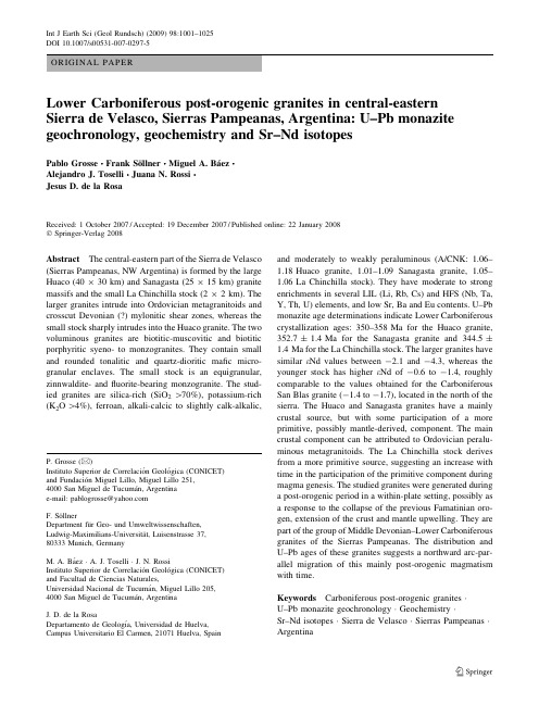
ORIGINAL PAPERLower Carboniferous post-orogenic granites in central-eastern Sierra de Velasco,Sierras Pampeanas,Argentina:U–Pb monazite geochronology,geochemistry and Sr–Nd isotopesPablo Grosse ÆFrank So¨llner ÆMiguel A.Ba ´ez ÆAlejandro J.Toselli ÆJuana N.Rossi ÆJesus D.de la RosaReceived:1October 2007/Accepted:19December 2007/Published online:22January 2008ÓSpringer-Verlag 2008Abstract The central-eastern part of the Sierra de Velasco (Sierras Pampeanas,NW Argentina)is formed by the large Huaco (40930km)and Sanagasta (25915km)granite massifs and the small La Chinchilla stock (292km).The larger granites intrude into Ordovician metagranitoids and crosscut Devonian (?)mylonitic shear zones,whereas the small stock sharply intrudes into the Huaco granite.The two voluminous granites are biotitic-muscovitic and biotitic porphyritic syeno-to monzogranites.They contain small and rounded tonalitic and quartz-dioritic mafic micro-granular enclaves.The small stock is an equigranular,zinnwaldite-and fluorite-bearing monzogranite.The stud-ied granites are silica-rich (SiO 2[70%),potassium-rich (K 2O [4%),ferroan,alkali-calcic to slightly calk-alkalic,and moderately to weakly peraluminous (A/CNK:1.06–1.18Huaco granite, 1.01–1.09Sanagasta granite, 1.05–1.06La Chinchilla stock).They have moderate to strong enrichments in several LIL (Li,Rb,Cs)and HFS (Nb,Ta,Y,Th,U)elements,and low Sr,Ba and Eu contents.U–Pb monazite age determinations indicate Lower Carboniferous crystallization ages:350–358Ma for the Huaco granite,352.7±1.4Ma for the Sanagasta granite and 344.5±1.4Ma for the La Chinchilla stock.The larger granites have similar e Nd values between -2.1and -4.3,whereas the younger stock has higher e Nd of -0.6to -1.4,roughly comparable to the values obtained for the Carboniferous San Blas granite (-1.4to -1.7),located in the north of the sierra.The Huaco and Sanagasta granites have a mainly crustal source,but with some participation of a more primitive,possibly mantle-derived,component.The main crustal component can be attributed to Ordovician peralu-minous metagranitoids.The La Chinchilla stock derives from a more primitive source,suggesting an increase with time in the participation of the primitive component during magma genesis.The studied granites were generated during a post-orogenic period in a within-plate setting,possibly as a response to the collapse of the previous Famatinian oro-gen,extension of the crust and mantle upwelling.They are part of the group of Middle Devonian–Lower Carboniferous granites of the Sierras Pampeanas.The distribution and U–Pb ages of these granites suggests a northward arc-par-allel migration of this mainly post-orogenic magmatism with time.Keywords Carboniferous post-orogenic granites ÁU–Pb monazite geochronology ÁGeochemistry ÁSr–Nd isotopes ÁSierra de Velasco ÁSierras Pampeanas ÁArgentinaP.Grosse (&)Instituto Superior de Correlacio´n Geolo ´gica (CONICET)and Fundacio´n Miguel Lillo,Miguel Lillo 251,4000San Miguel de Tucuma´n,Argentina e-mail:pablogrosse@F.So¨llner Department fu¨r Geo-und Umweltwissenschaften,Ludwig-Maximilians-Universita¨t,Luisenstrasse 37,80333Munich,GermanyM.A.Ba´ez ÁA.J.Toselli ÁJ.N.Rossi Instituto Superior de Correlacio´n Geolo ´gica (CONICET)and Facultad de Ciencias Naturales,Universidad Nacional de Tucuma´n,Miguel Lillo 205,4000San Miguel de Tucuma´n,Argentina J.D.de la RosaDepartamento de Geologı´a,Universidad de Huelva,Campus Universitario El Carmen,21071Huelva,SpainInt J Earth Sci (Geol Rundsch)(2009)98:1001–1025DOI 10.1007/s00531-007-0297-5IntroductionThe Sierras Pampeanas geological province of north-western Argentina contains abundant granitoid massifs generated during the Famatinian orogenic cycle(for details see Rapela et al.2001a;Miller and So¨llner2005).Most of these Famatinian granitoids are related to the main sub-duction phase of this cycle(e.g.Pankhurst et al.2000; Rapela et al.2001a;Miller and So¨llner2005)and have Early-Middle Ordovician ages(e.g.Pankhurst et al.1998, 2000;So¨llner et al.2001;Ho¨ckenreiner et al.2003) (Fig.1a).These granitoids are distributed along two sub-parallel,NNW–SSE trending belts:a main calc-alkaline I-type belt towards the southwest,and an inner peralumi-nous and S-type belt towards the northeast(Fig.1a).Additionally,numerous younger granites of Middle Devonian to Lower Carboniferous age are also present in the Sierras Pampeanas(e.g.Brogioni1987,1993;Rapela et al.1991;Grissom et al.1998;Llambı´as et al.1998; Saavedra et al.1998;Siegesmund et al.2004;Dahlquist et al.2006)(Fig.1a).The genesis of these granites is not well constrained,and they have been alternatively con-sidered as products of a crustal reheating process during a final phase of the Famatinian cycle,(e.g.Grissom et al. 1998;Llambı´as et al.1998;Ho¨ckenreiner et al.2003; Miller and So¨llner2005)or part of a separate cycle called Achalian(e.g.Sims et al.1998;Rapela et al.2001a; Siegesmund et al.2004;Lo´pez de Luchi et al.2007).The Sierra de Velasco is located in the central region of the Sierras Pampeanas(Fig.1a)and consists almost entirely of rocks of granitoid composition,making it the largest granitic massif of this geological province.The Sierra de Velasco granitoids have generally been regarded as part of the Famatinian inner peraluminous S-type belt (e.g.Rapela et al.1990;Toselli et al.1996,2000;Pank-hurst et al.2000),with the exception of the southern portion of the sierra which seems to correspond to the main calc-alkaline I-type belt(Bellos et al.2002;Bellos2005) (Fig.1a,b).However,field studies carried out in the northern(Ba´ez et al.2002;Ba´ez and Basei2005)and central(Grosse and Sardi2005;Grosse et al.2005)parts of the sierra indicate the presence of younger undeformed granites(Fig.1b),possibly belonging to the late-Famatin-ian,or Achalian,granite group.Recent U–Pb age determinations have confirmed that the northern unde-formed granites are of Lower Carboniferous age(Ba´ez et al.2004;Dahlquist et al.2006).The central undeformed granites have yet to be dated.The goal of this study is to determine the absolute ages and the geochemistry of the undeformed granites located in the central part of the Sierra de Velasco.To this end,we have carried out U–Pb dating on monazite and whole-rock elemental and Sr–Nd isotopic geochemical analyses.The obtained data are used to place constraints on the possible magma sources and geotectonic setting of these granites, and to discuss regional implications.Geological setting:the Sierra de VelascoThe Sierra de Velasco is dominated by rocks of granitoid composition.Low grade metamorphic rocks are only present as small outcrops along the easternflank of the sierra(Fig.1b,c).These phyllites and mica schists have been correlated with the La Ce´bila Formation,located in the Sierra de Ambato(Gonza´lez Bonorino1951;Espizua and Caminos1979).Recent discovery of marine fossils in this formation constrains its age to the Lower Ordovician (Verdecchia et al.2007),in agreement with detrital zircon geochronology(Rapela et al.2007).The granitoid units of the Sierra de Velasco have been reviewed and described by Toselli et al.(2000,2005)and Ba´ez et al.(2005).Two groups can be distinguished (Fig.1b):older deformed granitoids(here referred to as metagranitoids)and younger undeformed granites.The metagranitoids are the most abundant rocks.They are weakly to strongly foliated,depending on the degree of deformation.The main variety consists of strongly pera-luminous porphyritic two-mica-,garnet-,sillimanite-and kyanite-bearing meta-monzogranites(Rossi et al.2000, 2005).Subordinate varieties include strongly peraluminous porphyritic biotite–cordierite meta-monzogranites and moderately peraluminous coarse-to medium-grained bio-tite meta-granodiorites and meta-tonalites.In the southern part of the sierra,the main lithologies are metaluminous to weakly peraluminous biotite-hornblende meta-granodior-ites and meta-tonalites(Bellos2005)(Fig.1b).Two U–Pb SHRIMP determinations indicate Lower Ordovician ages for the metagranitoids(481±3Ma,Pankhurst et al.2000; 481±2Ma,Rapela et al.2001b).All of the metagranitoids are cut by several NNW–SSE trending mylonitic shear zones(Fig.1b).No age determi-nations exist of these shear zones in the Sierra de Velasco. However,similar mylonitic shear zones in other areas of the Sierras Pampeanas have been dated,with ages varying between the Upper Ordovician and the Upper Devonian (Northrup et al.1998;Rapela et al.1998;Sims et al.1998; Lo´pez et al.2000;Ho¨ckenreiner et al.2003).The precise Sm–Nd age of402±2Ma(Ho¨ckenreiner et al.2003) obtained on syntectonically grown garnet from mylonites of the Sierra de Copacabana(Fig.1a),which can be traced directly into the Sierra de Velasco(Lo´pez and Toselli 1993;So¨llner et al.2003),can be considered the best age estimate of mylonitization in this range.The undeformed granites crop out in the northern and central-eastern parts of the sierra(Fig.1b).Toselli et al.(2006)have grouped these granites in the Aimogasta batholith.The northern San Blas and Asha granites intrude the older metagranitoids and cross-cut the mylonitic shearzones (Ba´ez et al.2002;Ba ´ez and Basei 2005).They are moderately to weakly peraluminous porphyritic two-mica monzogranites.Existing U–Pb ages are 334±5Ma(conventional U–Pb method on zircon,Ba ´ez et al.2004)and 340±3Ma (U–Pb SHRIMP on zircon,Dahlquistet al.2006)for the San Blas granite,and 344±1Ma(conventional U–Pb method on monazite,Ba´ez et al.2004)for the Asha granite.In restricted areas,the granitic rocks are unconformably overlain by continental sandstones and conglomerates of the Paganzo Group (Salfity and Gorustovich 1984),ofFig.1a General geological map of the Sierras Pampeanas of NW Argentina with the main lithologies;sierras considered in the text are named.b General geology of the Sierra deVelasco;c Geological map of the central part of the Sierra de Velasco showing the Huaco,Sanagasta and La Chinchilla granites,with locations of dated samples;Bt biotite,Ms muscovite,Crd cordierite,Mzgr monzogranite,Ton tonalite,Grd granodioriteUpper Carboniferous to Permian age,deposited during regional uplift of the Sierras Pampeanas.Unconsolidated Tertiary-recent sediments,related to Andean tectonics, locallyfill basins and formfluvial terraces and cones. The Huaco,Sanagasta and La Chinchilla granitesThe central-eastern region of the Sierra de Velasco is formed mainly by two large granitic massifs,the Huaco granite(HG)and the Sanagasta granite(SG)(Fig.1c) (Grosse and Sardi2005).These granites consist of adjacent, sub-elipsoidal bodies with dimensions of approximately 40930km for the HG and25915km for the SG. Additionally,a small stock of around292km,named La Chinchilla stock(LCS),has been recognized in the central area of the HG(Fig.1c)(Grosse et al.2005).The HG and the SG intrude into the older metagranitoids and mylonites and are not deformed.The contacts are sharp and the granites truncate both the structures of the metag-ranitoids and the mylonitic shear zones,and contain enclaves of both of these host rocks.Thesefield relation-ships indicate that the granites are younger than both the crystallization of the metagranitoids and their deformation. The contact between the HG and the SG is irregular and transitional,suggesting that the two granites have similar ages and consist of two coeval magmatic pulses.The transitional area between the two granites is of*100–200m;in Fig.1c the contact between the granites was drawn along this transitional zone.The LCS clearly intrudes into the HG and is thus younger.The contacts are sharp and straight,and aplitic dykes from the LCS com-monly cut through the HG.Both the HG and the SG are rather homogeneous por-phyritic syeno-to monzogranites.They are characterized by abundant K-feldspar megacrysts up to12cm long (generally between2and5cm)set in a medium-to coarse-grained groundmass of quartz,plagioclase,K-feldspar, micas and accessory minerals.The megacrysts are usually oriented,defining a primary magmatic foliation.The HG consists in grayish-white K-feldspar megacrysts (30–36vol.%)and a groundmass of anhedral quartz(25–39%),subhedral plagioclase laths(An10–23)(18–31%), interstitial perthitic K-feldspar(2–14%),dark brown to straw-colored biotite(4–10%)and muscovite(2–6%). Accessory minerals include apatite(up to0.5%),zircon, monazite and ilmenite,all of which are generally associ-ated with,or included in,biotite.The SG contains pink K-feldspar megacrysts(33–37%) that are occasionally mantled by plagioclase generating a Rapakivi-like texture.The groundmass consists in anhedral quartz(23–34%),subhedral plagioclase laths(An18–24) (17–33%),interstitial perthitic K-feldspar(2–17%),and dark brown to straw-colored biotite(3–10%).Muscovite is absent or very scarce(0–2%).Accessory minerals are commonly found included in biotite.Apatite is less abundant than in the HG,whereas zircon,monazite and especially the opaque minerals(both ilmenite and magne-tite)are more frequent.In addition,titanite and allanite are sometimes present.Both the HG and the SG commonly contain small and rounded mafic microgranular enclaves.These generally have ovoid shapes,elongated parallel to the magmaticflow direction.The enclaves arefine-to veryfine-grained equigranular tonalites and quartz-diorites.They contain abundant biotite(15–50%)forming small,subhedral crys-tals.Opaque minerals and acicular apatite are common. The enclaves usually contain much larger xenocrysts of quartz,feldspar or biotite,and have chilled margins,sug-gesting partial assimilation and homogenization with the enclosing granites.Pegmatites and aplites are very common in these gran-ites,specially in the HG.The larger pegmatites are zoned and belong to the rare-element class,beryl type,beryl-columbite-phosphate sub-type with a hybrid LCT-NYF affiliation(Galliski1993;Sardi2005;Sardi and Grosse 2005).The HG also contains a small outcrop of an orbic-ular granite(Quartino and Villar Fabre1962;Grosse et al. 2006b).The LCS is a medium-grained,equigranular to slightly porphyritic,monzogranite.It shows a weak textural zona-tion determined by a progressive increase in grain size towards the center of the stock,where a slight porphyritic texture is present(up to10%of K-feldspar megacrysts). Mineralogically,the LCS consists of quartz(37–42%), plagioclase(almost pure albite,An1–2)(25–33%),K-feld-spar(19–34%),discolored,very pale brown to pale red-brown biotite(4–9%),anhedral and irregularly shaped fluorite(up to1%)and small quantities of zircon,monazite, opaque minerals and very scarce apatite.Beryl is occa-sionally present as euhedral prismatic crystals.Microprobe analyses(Grosse et al.2006a)indicate that the biotites of the HG and the SG have compositions ranging from Fe-biotites to siderophyllites(according to the classification diagram of Tischendorf et al.1997)and have high Fe/(Fe+Mg)ratios(0.76–0.82),typical of evolved granites.In the discrimination diagram of Nachit et al.(1985),they plot in the calc-alkalinefield.Biotites from de LCS have very high Fe/(Fe+Mg)ratios(0.94–0.97)and are Li-rich.They classify mainly as zinnwaldites and also as protolithionites in the classification diagram of Tischendorf et al.(1997).Zircons of the HG and the SG have similar morpholo-gies.They correspond mainly to the S17–19and S22–23 types of Pupin(1980),which are characteristic of calc-alkaline series granites.On the other hand,the zirconsof the LCS are different,with morphologies mostly of the P5-type of Pupin(1980),of primitive alkaline affiliation. The San Blas granite,in the north of the sierra(Fig.1b), has the same zircon typology as the LCS.No previous U–Pb age determinations exist of the HG and the SG,while the LCS has not been previously dated by any method.K–Ar and Rb–Sr geochronological studies have been carried out on granites of the Sierra de Velasco, which in some cases correspond to the HG or SG(see compilation in Linares and Gonza´lez1990).The ages in these studies are very variable,spanning from the Ordo-vician to the Permian,probably due to the inherent problems of the methods used(low closure temperature,Ar loss,etc.).Analytical methodsU–Pb geochronologyU–Pb geochronology was carried out at the Department of Earth-and Environmental Sciences,Ludwig-Maximilians-Universita¨t,Munich,Germany.Heavy mineral concen-trates,mainly zircons and monazites,were obtained using standard crushing,magnetic separation,and heavy-liquid techniques.For each analyzed sample around50monazite crystals were handpicked.Chosen crystals were yellow, translucent,anhedral to subhedral and lacked inclusions and fractures.We chose to analyze monazites because this mineral generally does not contain inherited cores and does not suffer radiogenic Pb loss at low temperatures,both common problems in zircons(see Parrish1990for discussion).Additionally,the closing temperature of monazite,although slightly lower than that of zircon(for details see Romer and Ro¨tzler2001),is sufficiently high to maintain the system unperturbed by low-temperature post-crystallization events.The monazite fractions were cleaned with purified6N HCl,H2O and acetone,and then deposited in Teflon inserts together with a mixed205Pb–233U spike.Subsequently, samples were dissolved in autoclaves,heated at180°C,for 5days using48%HF and subsequently6N HCl.The U and Pb of the samples were separated using small50l l ion exchange columns with Dowex raisin AG198100–200 mesh.The isotopic ratios of Pb and U were determined with a thermal ionization mass spectrometer(TIMS) Finnigan MAT261/262.Pb isotopes were measured in static mode and U isotopes in dynamic mode.Standards (NBS982Pb and U500)were used for measurement con-trol.U–Pb data was treated using the PBDAT1.24(Ludwig 1994)and ISOPLOT/Ex2.49x(Ludwig2001)programs. Errors quoted are at the2r confidence level.The correc-tions for initial non-radiogenic Pb was obtained following the model of Stacey and Kramers(1975).The U decay constants proposed by the IUGS(Steiger and Ja¨ger1977) were used for the age calculations.Mass fractionation was corrected using0.13±0.06%/a.m.u.for Pb and0.05±0.04%per a.m.u for U.Together with the samples,a procedural blank was analyzed to determine the level of contamination.For Pb blank corrections a mean value of 0.2ng and an isotopic composition of208Pb/204Pb=38.14; 207Pb/204Pb=15.63;206Pb/204Pb=18.15was used.Long term measured standards gave values of:NBS982(Pb): 208Pb/206Pb=0.99474±0.00013(0.013%,2rm,n=94); U500(U):238U/235U=1.00312±0.00027(=0.027%, 2r m,n=14).Whole-rock major and trace element geochemistry Whole-rock geochemistry was determined at the universi-ties of Oviedo(major elements)and Huelva(trace elements),Spain.Major elements were analyzed by X-ray fluorescence(XRF)with a Phillips PW2404system using glass beads.The typical precision of this method is better than±1.5%relative.Trace elements were analyzed by inductively coupled plasma mass spectrometry(ICP-MS) with an HP-4500system.Samples were dissolved using a mixture of HF+HNO3(8:3),a second dissolution in HNO3after evaporation andfinal dissolution in HCl.The precision and accuracy for most elements is between5and 10%relative(5–7%for Rb,Sr,Nd and Sm)and was controlled by repeated analyses of international rock stan-dards SARM-1(granite)and SARM-4(norite).Details on the method can be found in de la Rosa et al.(2001).Sr and Nd isotope geochemistrySr and Nd isotope analyses were carried out at the Department of Earth-and Environmental Sciences, Ludwig-Maximilians-Universita¨t,Munich,Germany.The analyzed powders were the same as those used for major and trace element analyses.For the determination of con-centrations and for comparison with the ICP-MS data,a mixed Sm–Nd spike was added to12samples.For the remaining samples,and for all Rb–Sr calculations,the concentrations obtained by ICP-MS were used.Samples(approximately0.1g each)were dissolved on a hot plate(140°C)during36h using a mixture of5ml of HF48%+HNO3(5:1).Sr and REE were separated using ion exchange columns with Dowex AG50W raisin.Nd and Sm were then separated from the total REE fractions using smaller ion exchange columns with bis(2-ethyl-hexyl)phosphoric acid(HDEHP)and Teflon powder.Theisotopic ratios of Sr,Nd and Sm were determined with a thermal ionization mass spectrometer (TIMS)Finnigan MAT 261/262.Standards were used for measurement control (NBS987,AMES Nd and AMES Sm).All errors used are at the 95%(2r )confidence level.Mass fraction-ation was corrected normalizing the isotopic ratios to 88Sr/86Sr =8.3752094for Sr,146Nd/144Nd =0.7219for Nd,and 148Sm/152Sm =0.4204548for Sm.CHUR con-stants used for e Nd calculation were 143Nd/144Nd =0.512638(Goldstein et al.1984)and 147Sm/144Nd =0.1967(Peucat et al.1988).One-step model ages were calculated following Goldstein et al.(1984)(with 143Nd/144Nd (DM)=0.51315and 147Sm/144Nd (DM)=0.217)and two-step model ages were calculated following Liew and Hofmann (1988)(with 143Nd/144Nd (DM)=0.513151,147Sm/144Nd (DM)=0.219and 147Sm/144Nd (CC)=0.12).During the period of analyses,the measured standards gave the following average values:NBS987(Sr):87Sr/86Sr =0.710230±0.000013(0.0018%,2r m ,n =8);AMES (Nd):143Nd/144Nd =0.512131±0.000007(0.0013%,2r m ,n =10);AMES (Sm):149Sm/147Sm =0.91262±0.00016(0.018%,2r m ,n =3).U–Pb monazite geochronologyMonazite fractions of six samples were analyzed,three of which correspond to the Sanagasta granite (SG),two to the Huaco granite (HG),and one to the La Chinchilla stock (LCS).Locations of the analyzed samples are shown in Fig.1c.Table 1shows the analytical results.In the U–Pb concordia diagram (Fig.2),two of the six analyzed samples are concordant whereas the other four are discordant,three of which plot above the concordia (phe-nomenon called ‘‘reverse discordance’’)and one below.Reverse discordance in monazite has been observed by many authors and seems to be a common phenomenon in this mineral (Parrish et al.1990,and references therein).Scha¨rer (1984)suggests that reverse discordances are owed to an excess in 206Pb due to the decay of 230Th,an inter-mediate product in the decay chain of 238U to 206Pb,incorporated in significant amounts in the crystal during crystallization of monazite,because this mineral is a carrier of Th.This might be valid for sample 7703Mo,which is slightly reverse discordant (Fig.2).However,samples 7365Mo,7381Mo and 7369Mo are strongly reverse and normally discordant,respectively (Fig.2).These samples probably suffered loss of U (7365Mo,7381Mo)and radiogenic Pb (7369Mo).The two samples of the HG are strongly reverse discor-dant,probably due to loss of U (U contents:6,135and 10,129ppm)(Fig.2).207Pb/206Pb ages of both samples are equivalent within limits of errors at 350±5andT a b l e 1U –P b m o n a z i t e d a t a o f t h e t h r e e s t u d i e d g r a n i t e s o f c e n t r a l -e a s t e r n S i e r r a d e V e l a s c oS a m p l eW e i g h t (g )U (p p m )T h (p p m )P b (p p m )206P b /204P b m e a s u r e dC a l c u l a t e d a t o m i c r a t i o sC a l c u l a t e d a g e s (i n M a )206P b /238U2r (%)207P b /235U2r(%)207P b /206P b2r (%)206P b /238U2r207P b /235U2r207P b /206P b2rH u a c o g r a n i t e7365M o0.0001521016983552159071340.068090.210.502170.250.053490.12424.60.9413.21.0349.75.37381M o 0.000138613546863146943430.113740.210.841770.240.053680.11694.41.5620.11.5357.54.9S a n a g a s t a g r a n i t e7369M o0.00011030483830554140230800.005920.210.043480.280.053300.1738.00.143.20.1341.57.87379M o0.000093331166434104940230.056270.210.414820.260.053470.15352.90.7352.30.9348.76.77703M o0.00015022266190997831150.056310.210.411960.330.053060.24353.20.7350.31.2331.311.0L a C h i n c h i l l a s t o c k7740M o 0.00012226816011092719720.054910.210.402970.330.053230.24344.60.7343.81.1338.610.9R a d i o g e n i c P b c o r r e c t e d f o r b l a n k a n d f o r i n i t i a l P b (f o l l o w i n g t h e m o d e l o f S t a c e y a n d K r a m e r s 1975).U c o r r e c t e d f o r b l a n k .A g e s c a l c u l a t e d u s i n g t h e P B D A T 1.24p r o g r a m (L u d w i g 1994)a n d t h e d e c a y c o n s t a n t s r e c o m m e n d e d b y t h e I U G S (S t e i g e r a n d J a¨g e r 1977)358±5Ma.These ages are interpreted as the best estimatefor crystallization of the HG.Recently,So¨llner et al.(2007)have carried out LA-ICP-MS U–Pb age determinations on zircons of sample 7365of the HG,obtaining a main crystallization age of 354±4Ma,thus confirming the monazite 207Pb/206Pb ages.In addition,many of these zir-cons have non-detrital inherited cores with Ordovician ages,suggesting significant participation of Ordovician metag-ranitoids in the formation of the HG (So¨llner et al.2007).Only one of the three samples of the SG (sample 7379Mo)gives a concordant age of 352.7±1.4Ma (degree of discordance =1.5%,Fig.2).Sample 7703Mo is slightly reverse discordant at 350.3±1.2Ma (207Pb/235U age),whereas sample 7369Mo is strongly discordant at 38.0±0.1Ma (206Pb/238U age;207Pb/206Pb age =342±8Ma)(Fig.2),suggesting loss of radiogenic Pb,possibly related to the very high measured U content (30,483ppm)and the presence of dim and/or fractured crystals.All three data points,including the origin,fit a regression line with an upper intercept of 340±26Ma (MSWD =3.8).The concordant age of 352.7±1.4Ma of sample 7379Mo is interpreted as the most precise and adequate age of crystallization of the SG.Sample 7740Mo of the LCS is concordant at 344.5±1.4Ma (degree of discordance =1.2%,Fig.2),which is interpreted as dating the time of crystallization of the LCS.GeochemistryMajor and trace elementsTable 2shows 31whole-rock major and trace element chemical analyses of the studied granites;13analysescorrespond to the HG,10to the SG,4to the LCS and 4to mafic microgranular enclaves of the HG and the SG (see also Grosse et al.2007).For comparison,the average composition of the border and central facies of the San Blas granite are also shown (calculated from 13analyses of Ba´ez 2006).The HG and the SG are characterized by a high and restricted SiO 2range of 69.7–74.7%(wt%).With slightly lower average SiO 2,the SG has somewhat higher Fe 2O 3tot ,MgO,TiO 2and CaO concentrations than the HG,although both granites are poor in these oxides.They are,on the other hand,rich in alkalis (generally [8%),specially in K 2O (generally [5%).Both granites are peraluminous;the HG is mainly moderately peraluminous (Alumina Satura-tion Index,A/CNK,= 1.06–1.18),whereas the SG is weakly peraluminous (A/CNK =1.01–1.09).In major element variation diagrams (Fig.3),both granites show similar,poorly defined correlations.Fe 2O 3tot ,MgO and TiO 2decrease with increasing SiO 2suggesting fractionation of mafic phases,mainly biotite.Al 2O 3,CaO and P 2O 5also decrease,suggesting fractionation of pla-gioclase and apatite,respectively,whereas Na 2O and K 2O do not correlate well with SiO 2.The HG and the SG can be distinguished well in an A/CNK versus SiO 2diagram (Fig.4a)and in the A–B diagram of Debon and Le Fort (1983)(Fig.4b),due to the different variations in peraluminosity:it decreases with differentia-tion in the HG,while it increases with differentiation in the SG.These opposite tendencies can be explained by frac-tionation of muscovite in the HG (which will strongly decrease the peraluminosity of the remaining melt due to its high peraluminosity)and the absence of this mineral in the SG (where the increase in peraluminosity is due mainly to the fractionation of plagioclase,whose A/CNK =1).Fig.2U–Pb Concordiadiagram of monazites from the three studied granites of central-eastern Sierra de Velasco.Two samples correspond to the Huaco granite (HG:7365Mo and 7381Mo),three to theSanagasta granite (SG:7369Mo,7379Mo and 7703Mo)and one to the La Chinchilla stock (LCS:7740Mo).See text for further explanations.Plotted errorellipses and quoted errors are at the 2r confidence level。

ρ常数263265″-回复Prelude: Understanding the Constant ρThe constant ρ, also known as the Greek letter rho, often appears in scientific equations to represent various concepts depending on the field of study. In physics, ρcan represent different physical quantities such as resistivity, density, and mass flow rate. In this article, we will explore the constant ρas it relates to density and delve into the significance of this value in different scientific contexts.Part 1: Definition and Significance of DensityDensity, represented by the symbol ρ, is a fundamental concept in physics and materials science. It is defined as the mass of an object divided by its volume. The density of a substance indicates how much mass is packed into a given volume of that substance.Mathematically, density is expressed as:ρ= m / VWhere:ρ- Densitym - MassV - VolumeDensity is measured in units such as kilograms per cubic meter (kg/m³) or grams per cubic centimeter (g/cm³). It is an essential characteristic of any material, as it determines its behavior under certain conditions.The density of a substance can provide crucial information about its composition, purity, and even its state of matter. For example, the density of a liquid can help determine its concentration or identify a particular substance in a mixture. In solid materials, density can indicate structural integrity or the presence of impurities.Part 2: Density in Different Scientific Fields2.1 PhysicsDensity plays a vital role in various areas of physics, including fluiddynamics, electromagnetism, and thermodynamics. In fluid dynamics, the density of a fluid influences its behavior, such as lift and drag forces in aerodynamics or buoyancy in fluid statics.2.2 Earth SciencesIn geophysics and geology, density is used to study the Earth's interior and differentiate between different layers. By analyzing density variations in the Earth's crust, scientists can gain insights into tectonic plate movements, mantle convection, and even predict volcanic eruptions.2.3 Material SciencesMaterial scientists rely on density measurements to identify and characterize materials. By comparing the density of an unknown material to that of known substances, scientists can determine its chemical composition or assess its quality and performance.Part 3: Application of ρConstant in Density CalculationsIn some cases, the constant ρis used within specific equations tocalculate density under specific conditions. Here are a few notable examples:3.1 ResistivityIn electrical engineering, the constant ρrepresents the resistivity of a material, denoted by the Greek letter rho (ρ). Resistivity measures how strongly a material opposes the flow of electric current. It is calculated as the product of the resistance of a conductor, its cross-sectional area, and ρ. The resistivity has units of ohm-meters (Ωm) and provides valuable information on a material's electrical conductivity and energy loss calculations.3.2 Atmospheric DensityIn meteorology and aerodynamics, the constant ρis used to describe atmospheric density, which relates to air pressure, temperature, and altitude. The ideal gas law equation, ρ= (P / R * T), incorporates the constant ρ. Here, P represents pressure, R the gas constant, and T temperature. Atmospheric density calculations are essential for weather prediction models, aircraft performance, and space exploration.Part 4: Conclusion and SummaryThe constant ρ, represented by the Greek letter rho, is a versatile fundamental value used in various scientific disciplines. Its most common application is in calculating density, a fundamental property of matter that characterizes the mass-to-volume relationship of a substance. The density of an object or material provides valuable insights into its composition, purity, and behavior under different conditions.Understanding the significance of density and the role of the constant ρallows scientists and engineers to make informed decisions, solve complex problems, and develop innovative solutions across multiple fields, including physics, earth sciences, and material sciences. The applications of ρextend beyond density calculations, with its utilization in resistivity calculations and atmospheric density formulae.From the depths of Earth's core to the outer reaches of the universe, the constant ρhelps unlock the secrets of the physical world,driving scientific advancements and enhancing our understanding of the universe in which we live.。

residue difference 残基变异英文版Residue Difference: The Science Behind the VariationIn the vast and intricate landscape of biology, the concept of residue difference, or residue variation, plays a pivotal role. At its core, residue difference refers to the alterations in the amino acid sequence of a protein. These changes, often subtle, can have profound effects on the protein's structure, function, and interactions with other molecules.To understand the significance of residue difference, it's essential to appreciate the fundamental building blocks of life: proteins. Proteins are complex molecules made up of amino acids, which are arranged in a specific sequence to form a unique three-dimensional structure. This structure determines the protein's function, whether it's enzymatic activity, structural support, or molecular signaling.When a residue difference occurs, it means that one or more amino acids in the protein sequence have been replaced, deleted, or inserted. These changes can be the result of natural genetic variation, mutations caused by environmental factors, or even artificial modifications in biotechnology.The impact of residue difference is multifaceted. On one hand, these variations can lead to the emergence of new properties and functions, allowing the protein to adapt to changing environmental conditions. For instance, certain mutations can enhance a protein's resistance to heat or chemicals, or even confer new binding capabilities.However, residue difference can also have negative consequences. Sometimes, these changes can disrupt the protein's structure, leading to loss of function or even the development of diseases. Many genetic diseases, such as sickle cell anemia and cystic fibrosis, are the result of specific residue differences that affect the normal function of essential proteins.The study of residue difference is not just limited to basic science. It has wide-ranging applications in biotechnology, medicine, and even agriculture. For instance, scientists can engineer proteins with desired properties by introducing specific residue differences. These modified proteins can then be used in a range of applications, from drug delivery to environmental cleanup.In conclusion, residue difference is a fundamental aspect of protein biology. It represents the dynamic nature of proteins, their ability to adapt and evolve in response to changing environments. Understanding the principles of residue difference is crucial for gaining insights into the functions and interactions of proteins, as well as for developing novel biotechnological applications.中文版残基变异：变异的科学在生物学广阔而复杂的领域中，残基变异这一概念扮演着关键的角色。

介观物理的英文精选英文介观物理的英文：Introduction to PhysicsPhysics, a fundamental branch of natural science, explores the nature and properties of matter, energy, space, and time. It delves into the innermost workings of the universe, from the smallest particles that constitute matter to the largest structures in the cosmos. This discipline aims to understand the underlying principles governing the behavior of these entities and their interactions.The journey of physics begins with the study of classical mechanics, which describes the motion of objects and the forces that act upon them. Newton's laws of motion, for instance, provide a foundation for understanding how objects move and interact with each other. As we delve deeper, we encounter the laws of thermodynamics, which govern the transfer of heat and the behavior of systems in terms of energy.The realm of electromagnetism opens up a new dimension in physics. Maxwell's equations, which unify electricity and magnetism, form the backbone of modern electronics and telecommunications. These equations explain how electromagnetic waves propagate, including visible light, radio waves, and even the gamma rays emitted by stars.The advent of quantum mechanics revolutionized our understanding of the subatomic world. This theory, developed in the early 20th century, describes the behavior of particles and systems at the atomic and molecular level. It introduces concepts such as wave-particle duality and quantum entanglement, which challenge our traditional understanding of reality.Moreover, the field of relativity, pioneered by Einstein, revolutionized our comprehension of space and time. His special theory of relativity described how the perception of space and time changes with the speed of an observer, while his general theory of relativity explained gravity as a manifestation of the curvature of spacetime.Modern physics is a vast and ever-expanding field, with new discoveries and theories constantly shaping our understanding of the universe. It is not just a subject confined to textbooks and laboratories; it is a tool that has revolutionized technology, medicine, and even our daily lives. From the smartphones we carry to the satellites orbiting the Earth, the principles of physics are everywhere, shaping our world in immeasurable ways.In conclusion, physics is a discipline that strives to unravel the mysteries of the universe, from the microcosm to the macrocosm. It is an exciting journey that challenges our imagination and pushes the boundaries of human knowledge. Through the study of physics, we gain a deeper understanding of the world we live in and the infinite possibilities that lie ahead.中文对照翻译：物理学导论物理学是自然科学的一个基本分支，探索物质、能量、空间和时间的性质和性质。