An Optimality-Theoretic Alternative to the Apparent Wh-Movement in Old Japanese

Contents摘要 (1)Abstract (1)Chapter 1 American Romanticism(1810--1865) (2)1.Background reasons (2)1.1 Politically this period was ripe (2)1.2 Economically American had never been wealthier (2)1.3 Culturally American own value emerged (2)2.Basic features and styles (2)2.1 Expressiveness (2)2.2 Imagination (2)2.3 Worship of nature (2)2.4 Simplicity (3)2.5 Cultural nationalism (3)2.6 Liberty,freedom,democracy and individualism (3)3.Influence (3)Chapter 2 American Realism(1865--1914) (3)1. Background changes (3)1.1 Politics (4)1.2 Economics (4)1.3 Cultural and social changes (4)2. Basic features and styles (4)2.1 Truthful description of the actualities of the real life andmaterial (4)2.2 Focus on ordinariness (4)3. Three dominant figures (4)4. Influence (5)Chapter 3 American Naturalism(1890--1914) (5)1. Background information (5)1.1 Cultural and Social Background (5)1.2 Religion and theoretical basis (5)2. Major ideas and features of Naturalism (5)2.1 Determinism (5)2.2 World: godless, indifferent, hostile (6)2.3 Style: scientific objectivity (6)2.4 Subjects and themes (6)3. A representative work that show the ideas and features above (6)3. Influence (6)Chapter 4 American Modernism(1914--1945) (6)1. Background information (6)1.1 Politics (6)1.2 Economy (7)1.3 Cultural and social background (7)2. Characteristics and features of Modernism (7)3. Major genres and a representative of each one (7)3.1 Modern poetry——Ezra Pound (7)3.2 Modern fiction——Ernest Hemingway (7)4. Influence (8)Chapter 5 American Postmodernism(1914--1945) (8)1. Background information (8)1.1 Politics (8)1.2 Economics (8)1.3 Social and international background (8)2. Characteristics and major features (8)2.1 Experimental writing techniques (8)2.3 Irony, playfulness and black humor (9)3.Influence (9)Bibliographies (9)摘要具有自身特点的新文学的出现，是一个国家真正形成的标志。

Econ 752Microeconomic Theory IIProfessor: Douglas NelsonOffice: Tilton 108 (Murphy Institute), Phone: 865-5317Office Hours: Tuesday and Thursday, 3:30-5:30Phone: 865-5317email: ******************Webpage: /~dnelson/This course provides an overview of equilibrium analysis for competitive markets. The course is organized in four sections. An introductory section illustrates the main themes of the course in simple partial and general equilibrium environments. The second part of the course develops the main positive results from abstract general equilibrium theory. The third and fourth part of the course introduces students to the analysis of general equilibrium systems. Specifically, part III introduces positive analysis in terms of comparative statics, while part IV introduces students to welfare economics.Evaluation: Your performance in this course will be evaluated on the basis of two examinations (worth 100 points each). All students are expected to do all the expected reading and actively participate in all classes.Readings and exercises for the course will be drawn from the following core texts: Andreu Mas-Colell, Michael Whinston, and Jerry Green (1995). Microeconomic Theory.New York: Oxford University Press. [MWG]Hal Varian (1992). Microeconomic Analysis. New York: Norton. [Varian]Eugene Silberberg and Wing Suen (2001). The Structure of Economics: A Mathematical Analysis. Boston: Irwin/McGraw Hill. [Silberberg and Suen]Alan Woodland (1982). International Trade and Resource Allocation. Amsterdam: North Holland.Gareth Myles (1995). Public Economics. Cambridge: Cambridge University Press.In addition, there will be a large number of articles available electronically.The main substantive material of this course has been covered in a number of excellent texts. On pure general equilibrium theory, at a relatively elementary level the following are excellent: Peter Newman (1965). The Theory of Exchange. Englewood Cliffs: Prentice-Hall.James Quirk and Rubin Saposnik (1968). Introduction to General Equilibrium Theoryand Welfare Economics. New York: McGraw Hill.Werner Hildenbrand and Alan Kirman (1988). Equilibrium Analysis: Variations onThemes by Edgeworth and Walras. Amsterdam: North-Holland.Ross Starr (1997). General Equilibrium Theory: An Introduction. Cambridge: CUP.Bryan Ellickson (1993). Competitive Equilibrium: Theory and Applications. Cambridge: CUP.Alan Kirman, ed. (1998). Elements of General Equilibrium Analysis. Oxford: Blackwell. At a more advanced level, the following are excellent:Kenneth Arrow and Frank Hahn (1971). General Competitive Analysis. Amsterdam:North-Holland.Lionel McKenzie (2002). Classical General Equilibrium Theory. Cambridge: MIT Press.Andreu Mas-Colell (1985). The Theory of General Equilibrium: A DifferentiableApproach. Cambridge: CUP/Econometric Society.Yves Balasko (1988). Foundations of the Theory of General Equilibrium. San Diego:Academic Press.C. Aliprantis,D. Brown, and O. Burkinshaw (1990). Existence and Optimality ofCompetitive Equilibrium. Berlin: Springer-Verlag.On the application to public economics, texts emphasizing modern general equilibrium methods include:David Starrett (1988). Foundations of Public Economics. Cambridge: CambridgeUniversity Press.Jean-Jacques Laffont (1988). Fundamentals of Public Economics. Cambridge: MIT Press.Roger Guesnerie (1995). A Contribution to the Pure Theory of Taxation. Cambridge:Cambridge University Press.On the application to trade:Avinash Dixit and Victor Norman (1980). Theory of International Trade. Cambridge:Cambridge University Press.Kar-yiu Wong (1995). International Trade in Goods and Factor Mobility. Cambridge:MIT Press.Those interested in computational methods of general equilibrium analysis may want to consult: John Shoven and John Whalley (1992). Applying General Equilibrium. Cambridge:Cambridge University Press.Victor Ginsburgh and Michiel Keyzer (1997). The Structure of Applied GeneralEquilibrium Models. Cambridge: MIT Press.Joseph Francois and Kenneth Reinert, eds. (1997). Applied Methods for Trade PolicyAnalysis: A Handbook. Cambridge: Cambridge University Press.Finally, for those with an interest in the historical and philosophical background to general equilibrium theory, the place to start is a series of excellent books by E. Roy Weintraub:E.R. Weintraub (1979). Microfoundations. Cambridge: CUP.E.R. Weintraub (1986). General Equilibrium Analysis: Essays in Appraisal. Cambridge:CUP.E.R. Weintraub (1991). Stabilizing Dynamics: Constructing Economic Knowledge.Cambridge: CUP.E.R. Weintraub (2002). How Economics Became a Mathematical Science. Durham: DukeUniversity Press.Examination format. Both exams will be made up of problems drawn from material covered in the lectures and reading. These problems will generally be in the nature of extensions of that material, not simply replication of the relevant content. Exams must be written in blue books, which you must supply.Policy on examinations. The midterm exam will be given on tba. Unless you have a standard university accepted excuse for missing the exam (e.g. health with standard university form), you must take the exams at their scheduled time. The final examination will only be given on the scheduled date: tba (there will be no exceptions so do not make travel plans that conflict with this).Policy on examinations. The midterm exam will be given on 9 March. Unless you have a standard university accepted excuse for missing the exam (e.g. health with standard university form), you must take the exams at their scheduled time. The final examination will only be given on the scheduled date: 10 May, 8:00-12:00 (there will be no exceptions so do not make travel plans that conflict with this).Econ 752SYLLABUS Fall 2006 Topic I. Introduction! Partial Equilibrium Analysis of Competitive Equilibrium# Varian, Chapter 13.# MWG, Chapter 10 a-d and f.! General Equilibrium: Applying Microeconomic Tools toMacroeconomic Questions, Pure Exchange# MWG, Chapter 15, sections a-b# Varian, Chapter 17 and section 21.1.# Shapley and Shubik (1977). “An Example of a Trading Economywith Three Competitive Equilibria”. Journal of Political Economy;V.85-#4, pp. 873-875.# Debreu and Scarf (1963). “A Limit Theorem on the Core of anEconomy”. International Economic Review; V.4-#3, pp. 235-246.# Aumann (1964). “Markets with a Continuum of Traders”.Econometrica; V.32-#1/2, pp. 39-50.# Shubik (1984). “Two-Sided Markets: The Edgeworth Game”.Chapter 10 of A Game Theoretic Approach to Political Economy.Cambridge: MIT Press, pp. 252-285. [optional]# Hildenbrand and Kirman (1988). “Introduction”. In EquilibriumAnalysis. Amsterdam: North-Holland, pp. 1-49. [optional] ! General Equilibrium: Applying Microeconomic Tools toMacroeconomic Questions, Simple Economies with Production# MWG, Chapter 15, section c.# Varian, Chapter 18.# Koopmans (1957). “Allocation of Resources and the Price System”.Essay 1 of Three Essays on the State of Economic Science. NewYork: McGraw Hill, pp. 3-126. [especially pp. 1-66.]Topic II. Pure General Equilibrium Theory! Characterizing Equilibrium and Proving Existence# MWG, Chapter 17, sections a-d and f, appendix B.# Geanakoplos (2003). “Nash and Walras Equilibrium via Brouwer”.Economic Theory; V.21-#2/3, pp. 585-603.# Debreu (1998). “Existence”. Chapter 2 in A.P. Kirman, ed.,Elements of General Equilibrium Analysis. Oxford: Basil Blackwell,pp. 10-37. [optional]! Problems/Extensions: Nonconvexities# MWG, Chapter 17, section I# Chipman (1970). “External Economies of Scale and CompetitiveEquilibrium”. Quarterly Journal of Economics; V.84-#3, pp. 347-363.# Mayer (1974). “Homothetic Production Functions and the Shape of the Production Possibility Locus”. Journal of Economic Theory; V.8-#2, pp. 101-110. [ERes]# Starrett (1971). “Fundamental Non-Convexities in the Theory ofExternalities”. Journal of Economic Theory; V.4-#2, pp. 180-199.[ERes]# Cornes (1980). “External Effects: An Alternative Formulation”.European Economic Review; V.14-#3, pp. 307-321. [optional]! Problems/Extensions: Uncertainty# Varian, Chapter 20.# MWG, Chapter 19# Hens (1998). “Incomplete Markets”. Chapter 5 in A.P. Kirman, ed., Elements of General Equilibrium Analysis. Oxford: Basil Blackwell,pp. 139-210. [optional]! General Equilibrium Comparative Statics?: The Sonnenschein-Debreu-Mantel Result# MWG, Chapter 17, section d-f.# Saari (1995). “The Mathematical Complexity of SimpleEconomies”. Notices of the American Mathematical Society; V.42-#2, pp. 222-230.# Kirman (1989). “The Intrinsic Limits of Modern Economic Theory: The Emperor Has No Clothes”. Economic Journal; V.99-#395, pp.126-139.# Sonnenschein (1973). “Do Walras' Indentity and ContinuityCharacterize the Class of Community Excess Demand Functions?”.Journal of Economic Theory; V.6-#4, pp. 345-354.# Debreu (1974). “Excess Demand Functions”. Journal ofMathematical Economics; V.1-#1, pp. 15-23. [optional]# Mantel (1979). “Homothetic Preferences and Community ExcessDemand Functions”. Journal of Economic Theory; V.12-#2, pp.197-201. [optional]# Mas-Colell (1977). “On the Equilibrium Price Set of an ExchangeEconomy”. Journal of Mathematical Economics; V.4-#2, pp.117-126. [optional]# Kemp and Shimomura (2002). “The Sonnenschein-Debreu-MantelProposition and the Theory of International Trade”. Review ofInternational Economics; V.10-#4, pp. 671-679. [optional]# Brown and Matzkin (1996). “Testable Restrictions on theEquilibrium Manifold”. Econometrica; V.64-#?, pp. 1249-1262.[optional]# Nachbar (2002). “General Equilibrium Comparative Statics”.Econometrica; V.70-#5, pp. 2065-2974. [optional]Midterm: Tuesday, 9 March.No Class: Thursday, 11 MarchTopic III. Applied General Equilibrium Theory: Positive Analysis ! Introduction to Comparative Statics for Applied GE# Silberberg and Suen, Chapter 18. [ERes]# Woodland (1982). “The Production Sector”. Chapter 3 ofInternational Trade and Resource Allocation. Amsterdam: North-Holland, pp. 39-65. [ERes]# MWG, Chapter 15, section d# Jones (1965). “The Structure of Simple General EquilibriumModels”. Journal of Political Economy; V.73-#6, pp. 557-572.[optional]# Mussa (1979). “The Two Sector Model in Terms of Its Dual: AGeometric Exposition”. Journal of International Economics; V.9-#4,pp. 513-526. [optional]# Hale, Lady, Maybee, and Quirk (1999). “The CompetitiveEquilibrium: Comparative Statics”. Chapter 7 in NonparametricComparative Statics and Stability. Princeton: Princeton UniversityPress, pp. 170-205. [optional]! Maximum Value Functions and Comparative Statics for GeneralEquilibrium Analysis# MWG, Chapter 17, section g# Woodland (1982). “Comparative Statics of the Production Sector”.Chapter 4 of International Trade and Resource Allocation.Amsterdam: North-Holland, pp. 67-103. [ERes]# Woodland (1982). “Intermediate Inputs and Joint Outputs”.Chapter 5 of International Trade and Resource Allocation.Amsterdam: North-Holland, pp. 105-146. [ERes]! Applied General Equilibrium Theory: The Stolper-SamuelsonTheorem, from 2 × 2 to m × n.# Chipman (1969). “Factor Price Equalization and the Stolper-Samuelson Theorem”. International Economic Review; V.10-#3, pp.399-406.# Jones and Scheinkman (1977). “The Relevance of the Two-SectorProduction Model in Trade Theory”. Journal of Political Economy;V.85-#5, pp. 909-935.# Ethier (1982). “The General Role of Factor Intensity in theTheorems of International Trade”. Economics Letters; V.10-#3/4, pp.337-342. [ERes]# Ethier (1984). “Higher Dimensional Issues in Trade Theory”. in R.Jones and P. Kenen, eds. Handbook of International Economics--Vol.1. Amsterdam: North-Holland, 131-184. [optional]Topic IV. Welfare Economics: Pure and Applied! Fundamental Theorems of Welfare Economics# Silberberg and Suen, Chapter 19, sections 1-3. [ERes]# MWG, Chapter 16# Hammond (1998). “The Efficiency Theorems and Market Failure”.Chapter 6 in A.P. Kirman, ed., Elements of General EquilibriumAnalysis. Oxford: Basil Blackwell, pp. 211-240. [ERes]! Applied Welfare Economics,1: Introduction# MWG, Chapter 10 e.# Silberberg and Suen, Chapter 19, section 7. [ERes]# Blackorby and Donaldson (1985). “Consumers’ Surpluses andConsistent Cost-Benefit Tests”. Social Choice and Welfare; V.1-#4,pp. 251-262. [optional]# Blackorby and Donaldson (1990). “The Case Against the Use ofthe Sum of Compensating Variations in Cost-Benefit Analysis”.Canadian Journal of Economics; V.23-#3, pp. 471-494.# Blackorby and Donaldson (1999). “Market Demand Curves andDupuit-Marshall Consumers’ Surpluses: A General EquilibriumAnalysis”. Mathematical Social Sciences; V37-#2, pp. 139-163.# Ahlheim (1998). “Measures of Economic Welfare”. In Barberà,Hammond, and Seidl, eds. Handbook of Utility Theory. Dordrecht:Kluwer, pp. 483-568. [Optional: covers one person theory]! Applied Welfare Economics, 2: Commodity Taxation# Myles, Chapter 4. [ERes]# Diamond and Mirrlees (1971). “Optimal Taxation and PublicProduction, I: Production Efficiency”. American Economic Review;V.61-#1, pp. 8-27. [optional]# Diamond and Mirrlees (1971). “Optimal Taxation and PublicProduction, II: Tax Rules”. American Economic Review; V.61-#3, pp.261-278. [optional]# Diamond and McFadden (1974). “Some Uses of the ExpenditureFunction in Public Finance”. Journal of Public Economics; V.3-#1,pp. 3-21.# Greenberg and Denzau (1988). “Profit and Expenditure Functionsin Basic Public Finance: An Expository Note”. Economic Inquiry;V.26-#1, pp. 145-158.# Deaton (1981). “Optimal Taxes and the Structure of Preferences”.Econometrica; V.49-#5, pp. 1245-1260.# Stern (1986). “A Note on Commodity Taxation: The Choice ofVariable and the Slutsky, Hessian and Antonelli Matrices (SHAM)”.Review of Economic Studies; V.53-#2, pp. 293-299.! Applied Welfare Economics, 3: Distortions, Second-best, and Policy# Silberberg and Suen, Chapter 19, sections 5 and 6. [ERes]# MWG, Chapter 22, sections a-d# Myles, Chapter 10. [ERes]# Hammond (1998). “The Efficiency Theorems and Market Failure”.Chapter 6 in A.P. Kirman, ed., Elements of General EquilibriumAnalysis. Oxford: Basil Blackwell, pp. 240-260. [ERes]# Hurwicz (1999). “Revisiting Externalities”. Journal of PublicEconomics Theory; V.1-#2, pp. 225-245.! Social Choice Theory: A (Very) Brief Introduction# MWG, Chapter 21# Fleurbaey and Mongin (2005). “The News of the Death of WelfareEconomics is Greatly Exaggerated”. Social Choice & Welfare;V.25-#2/3, pp. 381-418.# Mongin and d’Aspermont (1998). “Utility Theory and Ethics”. InBarberà, Hammond, and Seidl, eds. Handbook of Utility Theory.Dordrecht: Kluwer, pp. 371-481. [optional]Final Examination: 10 May, 8:00-12:00.。

顺应事情发展的客观规律英语作文Embracing the Immutable Laws of Nature.The universe operates according to an intricate tapestry of laws and principles, meticulously woven into the fabric of existence. These laws, like the unwavering force of gravity or the relentless passage of time, guide all that transpires, shaping the trajectories of both the celestial and the mundane. To live in harmony with the world around us, it is crucial that we align our actions and aspirations with these immutable laws.One of the most fundamental laws of nature is the principle of cause and effect. Every action, every thought, and every decision sets in motion a chain of consequences that reverberate through time. By understanding this law, we can act with greater foresight, weighing the potential outcomes of our choices and striving to sow seeds that will bear positive fruit.Another inviolable law is the law of impermanence. All things in the universe undergo constant flux and transformation, from the ceaseless cycles of day and nightto the birth and death of civilizations. By embracing this principle, we can learn to accept change with grace and resilience, recognizing that even in the face of adversity, there is always the potential for renewal and growth.The law of attraction is another potent force that shapes our lives. This law states that like attracts like, and that the energy we emit into the world will inevitably return to us. By cultivating positive thoughts, emotions, and intentions, we attract more of the same into our lives. Conversely, dwelling on negativity and fear can lead to a self-fulfilling cycle of unhappiness and misfortune.Understanding the laws of nature can also empower us to live more sustainable lives. The law of conservation of energy teaches us that energy can neither be created nor destroyed, only transformed from one form to another. By embracing this principle, we can make conscious choices to conserve resources and reduce our impact on the environment.The law of interdependence reminds us that all living beings are interconnected and interdependent. Our actions have consequences not only for ourselves but also for the wider ecosystem. By respecting nature and recognizing our role as stewards of the planet, we can help to create amore harmonious and sustainable world for ourselves and for generations to come.Embracing the laws of nature is not about denying free will or conforming to some predetermined destiny. Rather,it is about aligning our actions and intentions with the underlying principles that govern the universe. By doing so, we can live more meaningful, fulfilling, and sustainable lives, maximizing our potential while respecting the immutable forces that shape our existence.In the words of the ancient sage Lao Tzu, "The highest good is like water. Water gives life to the ten thousand things and does not strive. It flows in places men reject and so is like the Tao." May we all strive to embody the wisdom of water, flowing effortlessly with the currents oflife, in harmony with the immutable laws that guide our journey.。

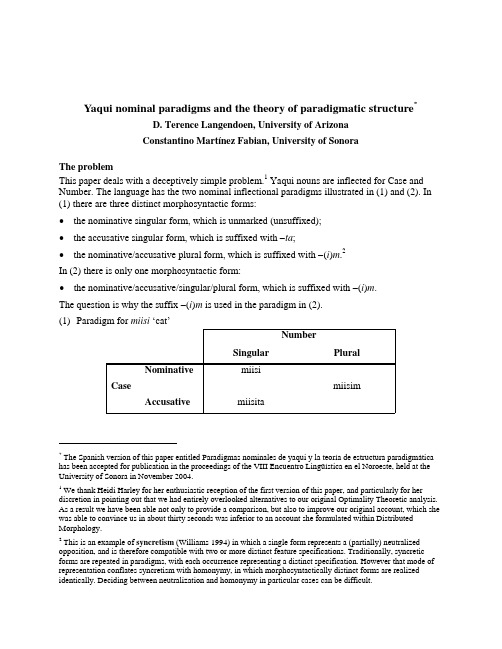
Yaqui nominal paradigms and the theory of paradigmatic structure*D. Terence Langendoen, University of ArizonaConstantino Martínez Fabian, University of SonoraThe problemThis paper deals with a deceptively simple problem.1 Yaqui nouns are inflected for Case and Number. The language has the two nominal inflectional paradigms illustrated in (1) and (2). In (1) there are three distinct morphosyntactic forms:•the nominative singular form, which is unmarked (unsuffixed);•the accusative singular form, which is suffixed with −ta;•the nominative/accusative plural form, which is suffixed with −(i)m.2In (2) there is only one morphosyntactic form:•the nominative/accusative/singular/plural form, which is suffixed with −(i)m.The question is why the suffix −(i)m is used in the paradigm in (2).(1)Paradigm for miisi ‘cat’NumberSingular PluralNominative miisimiisimCaseAccusative miisita* The Spanish version of this paper entitled Paradigmas nominales de yaqui y la teoría de estructura paradigmática has been accepted for publication in the proceedings of the VIII Encuentro Lingüística en el Noroeste, held at the University of Sonora in November 2004.1 We thank Heidi Harley for her enthusiastic reception of the first version of this paper, and particularly for her discretion in pointing out that we had entirely overlooked alternatives to our original Optimality Theoretic analysis. As a result we have been able not only to provide a comparison, but also to improve our original account, which she was able to convince us in about thirty seconds was inferior to an account she formulated within Distributed Morphology.2 This is an example of syncretism (Williams 1994) in which a single form represents a (partially) neutralized opposition, and is therefore compatible with two or more distinct feature specifications. Traditionally, syncretic forms are repeated in paradigms, with each occurrence representing a distinct specification. However that mode of representation conflates syncretism with homonymy, in which morphosyntactically distinct forms are realized identically. Deciding between neutralization and homonymy in particular cases can be difficult.(2)Paradigm for supe ‘shirt’NumberSingular PluralNominativesupemCaseAccusativeTypes of inflectional paradigmsTo answer this question, we need to describe in some detail the nature of inflectional paradigms.An inflectional paradigm is a nonempty set of inflections of a linguistic form or class of formsfor a nonempty set of inflectional features. Abstracting away from the morphosyntactic and morphophonological realization of these inflections, we obtain the notion of a schema for an inflectional paradigm, in which the members of the schema represent the various values of those features. Such a schema may be complete or defective. It is complete if all possible values forthose features are represented by a member of the schema; otherwise it is defective.Complete schemas for inflectional paradigmsFor example, suppose, as in Yaqui, there is a class of forms that is inflected for the features Caseand Number, where Case takes the binary values [Nominative] and [Accusative], and Numberthe binary values [Singular] and [Plural]. Then there are 24− 1 = 15 schemas of complete inflectional paradigms for those features, depending on whether any of the feature-valuedistinctions are neutralized, and if so which ones. The 15 schemas are shown in (3) through (17). Yaqui manifests two of these 15 schemas; the paradigm in (1) is an instance of the schema in (4),and the paradigm in (2) is an instance of the schema in (17).(3)Non-neutralized (full) complete paradigmatic schema for binary Case and Number featuresNumberSingular Plural Nominative [Nominative] & [Singular] [Nominative] & [Plural] CaseAccusative [Accusative] & [Singular] [Accusative] & [Plural](4)Neutralization of Case with [Plural]NumberSingular Plural Nominative [Nominative] & [Singular]CaseAccusative [Accusative] & [Singular][Plural](5)Neutralization of Case with [Singular]NumberSingular Plural Nominative [Nominative] & [Plural]CaseAccusative [Singular][Accusative] & [Plural](6)Neutralization of Number with [Accusative]NumberSingular Plural Nominative [Nominative] & [Singular] [Nominative] & [Plural] CaseAccusative [Accusative](7)Neutralization of Number with [Nominative]NumberSingular Plural Nominative [Nominative]CaseAccusative [Accusative] & [Singular] [Accusative] & [Plural](8)Partial neutralization of Case and Number along NW−SE diagonalNumberSingular Plural[Nominative] & [Plural]Nominative([Nominative] & [Singular]) | ([Accusative] & [Plural]) CaseAccusative [Accusative] & [Singular](9)Partial neutralization of Case and Number along SW−NE diagonalNumberSingular Plural[Nominative] & [Singular]Nominative([Accusative] & [Singular]) | ([Nominative] & [Plural]) CaseAccusative [Accusative] & [Plural](10)Complete neutralization of CaseNumberSingular Plural Nominative[Singular] [Plural]CaseAccusative(11)Complete neutralization of NumberNumberSingular Plural Nominative [Nominative]CaseAccusative [Accusative](12)Neutralization through negation of [Nominative] & [Singular]NumberSingular Plural Nominative [Nominative]&[Singular]↑CaseAccusative ←~ ([Nominative]&[Singular])(13)Neutralization through negation of [Accusative] & [Singular]NumberSingular Plural Nominative ←~ ([Accusative]&[Singular])↓CaseAccusative [Accusative]&[Singular](14)Neutralization through negation of [Nominative] & [Plural]NumberSingular PluralNominative↑[Nominative]&[Plural]CaseAccusative ~ ([Nominative]&[Plural]) →(15)Neutralization through negation of [Accusative] & [Plural]NumberSingular PluralNominative ~ ([Accusative]&[Plural])↓→CaseAccusative [Accusative]&[Plural](16)Neutralization along both diagonalsNumberSingular Plural Nominative([Accusative] & [Singular]) | ([Nominative] & [Plural]) Case([Nominative] & [Singular]) | ([Accusative] & [Plural])Accusative(17)Full neutralization of Case and NumberNumberSingular Plural Nominative[ ]CaseAccusativeDefective schemas for inflectional paradigmsA defective schema for inflectional paradigms, on the other hand, is one whose members do notcover the space of all possible values for the features involved, i.e. one that leaves a “gap”. For example, corresponding to the full complete schema in (3), there is the defective schema in (18)that has no provision for the [Accusative] & [Plural] combination of values. In general there aremany more defective schemas for inflectional paradigms than complete ones; for example, thereare 36 defective schemas for two binary features compared to 15 complete ones, but theoccurrence of defective paradigms in natural language descriptions is comparatively rare. Weleave the explanation for this fact for another occasion; for now we simply declare that grammars abhor defective paradigms.(18)Defective schema for an inflectional paradigm, lacking [Accusative] & [Plural]NumberSingular Plural Nominative [Nominative] & [Singular] [Nominative] & [Plural] CaseAccusative [Accusative] & [Singular] −−The realization of complete paradigm schemasDifferent languages manifest different paradigm schemas for given sets of features, but certain preferences are clear. For example, we are aware of no cases in which the schemas involving the “diagonal” neutralizations such as (8), (9) and (16) are realized. In addition, schemas involving the negation of a particular combination of features such as (12)−(15) are unusual, an example is the Person and Number paradigm for the present tense of verbs (other than be) in standard English. On the other hand, schemas involving the neutralization of one or more features such as (4)−(7), (10) and (11) are quite commonly manifested, with preferences for which feature(s) to neutralize being dictated by markedness considerations. Finally, full complete schemas such as (3) are also very common, at least when the number of feature-value combinations is relatively small, as are fully neutralized complete schemas such as (17).Accounting for the Yaqui nominal paradigmsThere are two classes of morphological theories that account for paradigmatic patterns such as observed in Yaqui nominal inflection, those that are paradigm-based and those that are vocabulary-based (Bobaljik 2001: 53-54).3 An example of a vocabulary-based morphological theory is Distributed Morphology (DM) (Halle & Marantz 1993), which Bobaljik also espouses. An example of a paradigm-based theory is one developed by Edwin Williams, according to which a paradigm is “a real object, and not the epiphenomenal product of various rules” (Williams 1994: 22).A Distributed Morphology accountAn elegant DM account of the Yaqui nominal paradigms in (1) and (2) was suggested to us by Heidi Harley (see fn. 1). It goes as follows. Assume as we have already done that Yaqui nouns are inflected for Case and Number, that the values for Case are [Nominative] and [Accusative] and that the values for Number are [Singular] and [Plural]. Assume also that there are two classes of nouns, Class1 the miisi class and Class2 the supe class. Then the ordered list of morpheme realization rules in (19) derives the paradigms in (1) and (2), i.e. treats them precisely as epiphenomenal products.(19)Morpheme realization rules that derive the Yaqui nominal paradigms-ta ⇔ [Accusative] & [Singular] / Class1 ___-∅⇔ [Singular] / Class1 ___-(i)m ⇔ elsewhereThere are two noteworthy properties of this account. First, a zero affix must be postulated, since the rule for its insertion is ordered after that of -ta insertion and before the default insertion of-(i)m. Second, -(i)m has no inherent features; in particular it is not specified [Plural].3 Bobaljik (2001: 78, fn. 1) points out that certain morphological theories, such as that of Wunderlich (1995) and Stump (2001), may not be easily placed within one or the other of these classes.An Optimality Theory accountDM is a theory that ranks rules. On the other hand, Optimality Theory (OT), which ranks constraints rather than rules, can be used within the paradigm-based framework to account for the forms that appear in the paradigms in (1) and (2), but without the use of zero affixes or default (elsewhere) conditions. The suffix -(i)m may be assumed to be specified [Plural] and the suffix -ta specified as [Accusative]. Then, assuming that the entries in the paradigm schema in (4) appear in inputs together with a Class 1 noun such as miisi, we correctly account for the choice of affix in accordance with a faithfulness constraint we call F AITH FS (FS for “feature specifications”), as shown in the tableaux in (20)-(22).(20)Choice of miisi to represent miisi [Nominative] & [Singular]miisi [Nominative] & [Singular] F AITH FS⇒miisi **[Accusative] ***!miisi-ta[Plural] ***!miisi-m(21)Choice of miisi-ta to represent miisi [Accusative] & [Singular]miisi [Accusative] & [Singular] F AITH FSmiisi **!⇒miisi-ta [Accusative] *miisi-m[Plural] **!*(22)Choice of miisi-m to represent miisi [Plural]miisi [Plural] F AITH FSmiisi *!miisi-ta[Accusative] *!*⇒miisi-m [Plural]However, F AITH FS by itself does not predict that the affix -(i)m appears in instances of the paradigm schema (17). Instead, as shows, it predicts that no affix appears.(23)False prediction that supe represents supe [ ]supe [ ] F AITH FS/⇒supe[Accusative] *!supe-ta[Plural] *!supe-mTo force the choice of supem, several additional constraints are required. First, we need a constraint that prefers outputs of inflected forms that have affixes. Call that constraint H AVE A FF.Clearly F AITH FS >> H AVE A FF, since otherwise the choice of miisi as the expression of miisi [Nominative] & [Accusative] would be prevented. However, for Class2 nouns, we require in effect that H AVE A FF outrank F AITH FS. Whether this is a case of local reranking or an additional constraint expressed as a conditional is not our concern here. We assume the latter, calling the constraint H AVE A FF2, and proposing the ranking H AVE A FF2 >> F AITH FS >> H AVE A FF. Now, supe is not winning candidate for expressing supe [ ], but as (24) shows, we are still left with no basis for choosing between supe-ta and supe-m.(24)Failure to choose between supe-ta and supe-m as representing supe [ ]supe [ ] H AVE A FF2 F AITH FS H AVE A FFsupe *! */⇒supe-ta [Accusative] *⇒supe-m [Plural] *To account for the choice of supe-m, we propose two additional markedness filters: *C ASE, which indicates an aversion to marking Case, and *N UMBER, which indicates an aversion to marking Number, and the ranking F AITH FS >> *C ASE >> *N UMBER. Then, as (25) shows, we obtain the result that supem instantiates paradigm schema (17) in Yaqui.(25)Choice of supe-m to represent supe [ ]supe [ ] H AVE A FF2 F AITH FS *C ASE *N UMBER H AVE A FF supe *! *supe-ta[Accusative] * *!⇒supe-m [Plural] * *Comparison of DM and OT accounts of Yaqui nominal paradigmatic structureFrom our presentation so far of the DM and OT accounts of the paradigmatic structure of Yaqui nominals, one might conclude that the DM account is to be preferred on grounds of simplicity. As Bobaljik (2001) points out, a vocabulary-based account such as DM is conceptually simpler than paradigm-based accounts of morphological structure, so is to be preferred for that reason, all things being equal. Since we are interested not so much in the comparison between vocabulary-based and paradigm-based accounts as in the comparison of DM and OT accounts of paradigmatic structure, we now convert the paradigm-based OT account given above to a vocabulary-based one, so as to level the playing field for evaluating those two theories in this arena. To effect this conversion, we replace the inputs with elements that represent all possible combinations of the case and number feature values that Yaqui nouns can express and determine the constraint rankings that yield the correct outputs. For example, we consider an input such as miisi [Nominative] & [Plural] and determine what constraint ranking yields the desired miisi-m as output. For Class1 nouns, we determine immediately that the ranking F AITH FS >> *C ASE >> *N UMBER yields the desired outputs for all combinations of feature values. In (26) and (27), we give two illustrative tableaux.(26)Choice of miisi to express miisi [Nominative] & [Singular]miisi [Nominative] & [Singular] F AITH FS *C ASE *N UMBER⇒miisi **[Accusative] ***! *miisi-tamiisi-m[Plural] ***! *(27)Choice of miisi-m to express miisi [Accusative] & [Plural]miisi [Accusative] & [Plural] F AITH FS *C ASE *N UMBERmiisi **![Accusative] * *!miisi-ta⇒miisi-m [Plural] * *However, this ranking gives the same results for Class2 nouns as for Class1 nouns. In order that supe-m is always selected as output, no matter what feature value combinations are associated with the input stem supe, we require a version of the *C ASE constraint, call it *C ASE2, that is specific to Class2 nouns, with the ranking *C ASE2 >> F AITH FS; (28) shows that it does not matter how *C ASE2 is ranked with respect to H AVE A FF2.(28)Choice of supe-m to express supe [Accusative] & [Singular]supe [Accusative] & [Singular] H AVE A FF2 *C ASE2 F AITH FS *C ASE *N UMBER supe *![Accusative] *! * *supe-ta⇒supe-m [Plural] *** *The OT analysis presented in this section, like the DM analysis in the preceding section, is vocabulary-based, and derives the two Yaqui nominal paradigm schemas in (4) and (17). However, unlike the DM analysis, it assigns feature content to the suffix -(i)m, namely [Plural]; assigns only one feature value to -ta instead of two and does not explicitly restrict its occurrence to Class1 nouns; and does not posit a zero-affix, much less assign feature content to it. Moreover the association of features with Yaqui affixes is lexical, as proposed in Lieber (1982) and DiSciullo & Williams (1987), as opposed to realizational as in DM theories generally, and also in Williams (1994); see Bobaljik (2001: 56) for discussion. In all these respects, we believe that the OT analysis is closer to the ‘truth’ regarding Yaqui (and universal) grammar than the DM analysis. On the other hand, the DM analysis is simpler, inasmuch as it posits only three rules as opposed to the five constraints in the OT analysis. However, the DM theory suffers from the fact that there is an equally simple analysis in which the first two rules are reordered, given in (29), and there is no basis for choosing between them.Langendoen & Martínez, Yaqui nominal paradigms and the theory of paradigmatic structure 11(29)Another list of morpheme realization rules that derives the Yaqui nominal paradigms-∅⇔ [Nominative] & [Singular] / Class1 ___-ta ⇔ [Singular] / Class1 ___-(i)m ⇔ elsewhereFinally, another advantage we see to the OT analysis is that it provides the beginning of a basis for the analysis of the class of possible paradigms within the enormous space of paradigm schemas provided by the free combination of morphosyntactic feature values. Paradigm schema (4) is derived, as we have already seen, from the ranking F AITH FS >> *C ASE >> *N UMBER. Paradigm schema (17) with the [Plural] affix used throughout is derived from the rankingH AVE A FF >> *C ASE >> F AITH FS >> *N UMBER. The need to double the *C ASE and H AVE A FF constraints in the analysis of Yaqui results from having two coexisting nominal paradigms in the language.ReferencesBobaljik, Jonathan David (2001). Syncretism without paradigms: Remarks on Williams 1981, 1994. Yearbook of Morphology 2001: 53-85.DiSciullo, Anna Marie & Edwin Williams (1987). On the Definition of Word. Cambridge, MA: MIT Press.Halle, Morris & Alec Marantz (1993). Distributed morphology and the pieces of inflection. In Ken Hale & Samuel Jay Keyser (eds.), The View from Building 20: Essays in Linguistics in Honor of Sylvain Bromberger. Cambridge, MA: MIT Press, 111-176.Lieber, Rochelle (1982). Allomorphy. Linguistic Analysis 10: 27-52.Stump, Gregory T. (2001). Inflectional Morphology: A Theory of Paradigm Structure.Cambridge: Cambridge University Press.Williams, Edwin (1994). Remarks on lexical knowledge. Lingua 92: 7-34.Wunderlich, Dieter (1995). Minimalist morphology: The role of paradigms. Yearbook of Morphology 1995: 93-114.。

Deterministic Policy Gradient AlgorithmsDavid Silver DAVID@ DeepMind Technologies,London,UKGuy Lever GUY.LEVER@ University College London,UKNicolas Heess,Thomas Degris,Daan Wierstra,Martin Riedmiller*@ DeepMind Technologies,London,UKAbstractIn this paper we consider deterministic policygradient algorithms for reinforcement learningwith continuous actions.The deterministic pol-icy gradient has a particularly appealing form:itis the expected gradient of the action-value func-tion.This simple form means that the deter-ministic policy gradient can be estimated muchmore efficiently than the usual stochastic pol-icy gradient.To ensure adequate exploration,we introduce an off-policy actor-critic algorithmthat learns a deterministic target policy from anexploratory behaviour policy.We demonstratethat deterministic policy gradient algorithms cansignificantly outperform their stochastic counter-parts in high-dimensional action spaces.1.IntroductionPolicy gradient algorithms are widely used in reinforce-ment learning problems with continuous action spaces.The basic idea is to represent the policy by a parametric prob-ability distributionπθ(a|s)=P[a|s;θ]that stochastically selects action a in state s according to parameter vectorθ. Policy gradient algorithms typically proceed by sampling this stochastic policy and adjusting the policy parameters in the direction of greater cumulative reward.In this paper we instead consider deterministic policies a=µθ(s).It is natural to wonder whether the same ap-proach can be followed as for stochastic policies:adjusting the policy parameters in the direction of the policy gradi-ent.It was previously believed that the deterministic pol-icy gradient did not exist,or could only be obtained when using a model(Peters,2010).However,we show that the deterministic policy gradient does indeed exist,and further-more it has a simple model-free form that simply follows the gradient of the action-value function.In addition,we show that the deterministic policy gradient is the limiting Proceedings of the31st International Conference on Machine Learning,Beijing,China,2014.JMLR:W&CP volume32.Copy-right2014by the author(s).case,as policy variance tends to zero,of the stochastic pol-icy gradient.From a practical viewpoint,there is a crucial difference be-tween the stochastic and deterministic policy gradients.In the stochastic case,the policy gradient integrates over both state and action spaces,whereas in the deterministic case it only integrates over the state space.As a result,computing the stochastic policy gradient may require more samples, especially if the action space has many dimensions.In order to explore the full state and action space,a stochas-tic policy is often necessary.To ensure that our determinis-tic policy gradient algorithms continue to explore satisfac-torily,we introduce an off-policy learning algorithm.The basic idea is to choose actions according to a stochastic behaviour policy(to ensure adequate exploration),but to learn about a deterministic target policy(exploiting the ef-ficiency of the deterministic policy gradient).We use the deterministic policy gradient to derive an off-policy actor-critic algorithm that estimates the action-value function us-ing a differentiable function approximator,and then up-dates the policy parameters in the direction of the approx-imate action-value gradient.We also introduce a notion of compatible function approximation for deterministic policy gradients,to ensure that the approximation does not bias the policy gradient.We apply our deterministic actor-critic algorithms to sev-eral benchmark problems:a high-dimensional bandit;sev-eral standard benchmark reinforcement learning tasks with low dimensional action spaces;and a high-dimensional task for controlling an octopus arm.Our results demon-strate a significant performance advantage to using deter-ministic policy gradients over stochastic policy gradients, particularly in high dimensional tasks.Furthermore,our algorithms require no more computation than prior meth-ods:the computational cost of each update is linear in the action dimensionality and the number of policy parameters. Finally,there are many applications(for example in robotics)where a differentiable control policy is provided, but where there is no functionality to inject noise into the controller.In these cases,the stochastic policy gradient is inapplicable,whereas our methods may still be useful.2.Background2.1.PreliminariesWe study reinforcement learning and control problems in which an agent acts in a stochastic environment by sequen-tially choosing actions over a sequence of time steps,in order to maximise a cumulative reward.We model the problem as a Markov decision process (MDP)which com-prises:a state space S ,an action space A ,an initial state distribution with density p 1(s 1),a stationary transition dy-namics distribution with conditional density p (s t +1|s t ,a t )satisfying the Markov property p (s t +1|s 1,a 1,...,s t ,a t )=p (s t +1|s t ,a t ),for any trajectory s 1,a 1,s 2,a 2,...,s T ,a T in state-action space,and a reward function r :S ×A →R .A policy is used to select actions in the MDP.In general the policy is stochastic and denoted by πθ:S →P (A ),where P (A )is the set of probability measures on A and θ∈R n is a vector of n parameters,and πθ(a t |s t )is the conditional probability density at a t associated with the policy.The agent uses its policy to interact with the MDP to give a trajectory of states,actions and rewards,h 1:T =s 1,a 1,r 1...,s T ,a T ,r T over S ×A ×R .Thereturn r γtis the total discounted reward from time-step t onwards,r γt = ∞k =t γk −tr (s k ,a k )where 0<γ<1.Value functions are defined to be the expected total dis-counted reward,V π(s )=E [r γ1|S 1=s ;π]and Q π(s,a )=E [r γ1|S 1=s,A 1=a ;π].1The agent’s goal is to obtain a policy which maximises the cumulative discounted reward from the start state,denoted by the performance objectiveJ (π)=E [r γ1|π].We denote the density at state s after transitioning for t time steps from state s by p (s →s ,t,π).We also denote the (improper)discounted state distribution by ρπ(s ):= S∞t =1γt −1p 1(s )p (s →s ,t,π)d s .We can then write the performance objective as an expectation,J (πθ)= Sρπ(s )Aπθ(s,a )r (s,a )d a d s=E s ∼ρπ,a ∼πθ[r (s,a )](1)where E s ∼ρ[·]denotes the (improper)expected value with respect to discounted state distribution ρ(s ).2In the re-mainder of the paper we suppose for simplicity that A =R m and that S is a compact subset of R d .2.2.Stochastic Policy Gradient TheoremPolicy gradient algorithms are perhaps the most popular class of continuous action reinforcement learning algo-rithms.The basic idea behind these algorithms is to adjust1To simplify notation,we frequently drop the random vari-able in the conditional density and write p (s t +1|s t ,a t )=p (s t +1|S t =s t ,A t =a t );furthermore we superscript value functions by πrather than πθ.2The results in this paper may be extended to an average re-ward performance objective by choosing ρ(s )to be the stationary distribution of an ergodic MDP.the parameters θof the policy in the direction of the perfor-mance gradient ∇θJ (πθ).The fundamental result underly-ing these algorithms is the policy gradient theorem (Suttonet al.,1999),∇θJ (πθ)= Sρπ(s )A∇θπθ(a |s )Q π(s,a )d a d s=E s ∼ρπ,a ∼πθ[∇θlog πθ(a |s )Q π(s,a )](2)The policy gradient is surprisingly simple.In particular,despite the fact that the state distribution ρπ(s )depends on the policy parameters,the policy gradient does not depend on the gradient of the state distribution.This theorem has important practical value,because it re-duces the computation of the performance gradient to a simple expectation.The policy gradient theorem has been used to derive a variety of policy gradient algorithms (De-gris et al.,2012a ),by forming a sample-based estimate of this expectation.One issue that these algorithms must ad-dress is how to estimate the action-value function Q π(s,a ).Perhaps the simplest approach is to use a sample return r γt to estimate the value of Q π(s t ,a t ),which leads to a variant of the REINFORCE algorithm (Williams ,1992).2.3.Stochastic Actor-Critic AlgorithmsThe actor-critic is a widely used architecture based on the policy gradient theorem (Sutton et al.,1999;Peters et al.,2005;Bhatnagar et al.,2007;Degris et al.,2012a ).The actor-critic consists of two eponymous components.An ac-tor adjusts the parameters θof the stochastic policy πθ(s )by stochastic gradient ascent of Equation 2.Instead of the unknown true action-value function Q π(s,a )in Equation 2,an action-value function Q w (s,a )is used,with param-eter vector w .A critic estimates the action-value function Q w (s,a )≈Q π(s,a )using an appropriate policy evalua-tion algorithm such as temporal-difference learning.In general,substituting a function approximator Q w (s,a )for the true action-value function Q π(s,a )may introduce bias.However,if the function approximator is compati-ble such that i)Q w (s,a )=∇θlog πθ(a |s ) w and ii)the parameters w are chosen to minimise the mean-squareder-ror 2(w )=E s ∼ρπ,a ∼πθ (Q w (s,a )−Q π(s,a ))2,then there is no bias (Sutton et al.,1999),∇θJ (πθ)=E s ∼ρπ,a ∼πθ[∇θlog πθ(a |s )Q w (s,a )](3)More intuitively,condition i)says that compatible function approximators are linear in “features”of the stochastic pol-icy,∇θlog πθ(a |s ),and condition ii)requires that the pa-rameters are the solution to the linear regression problem that estimates Q π(s,a )from these features.In practice,condition ii)is usually relaxed in favour of policy evalu-ation algorithms that estimate the value function more ef-ficiently by temporal-difference learning (Bhatnagar et al.,2007;Degris et al.,2012b ;Peters et al.,2005);indeed ifboth i)and ii)are satisfied then the overall algorithm is equivalent to not using a critic at all (Sutton et al.,2000),much like the REINFORCE algorithm (Williams ,1992).2.4.Off-Policy Actor-CriticIt is often useful to estimate the policy gradient off-policy from trajectories sampled from a distinct behaviour policy β(a |s )=πθ(a |s ).In an off-policy setting,the perfor-mance objective is typically modified to be the value func-tion of the target policy,averaged over the state distribution of the behaviour policy (Degris et al.,2012b ),J β(πθ)=S ρβ(s )V π(s )d s= SAρβ(s )πθ(a |s )Q π(s,a )d a d sDifferentiating the performance objective and applying an approximation gives the off-policy policy-gradient (Degris et al.,2012b )∇θJ β(πθ)≈ SAρβ(s )∇θπθ(a |s )Q π(s,a )d a d s (4)=E s ∼ρβ,a ∼βπθ(a |s )βθ(a |s )∇θlog πθ(a |s )Q π(s,a ) (5)This approximation drops a term that depends on the action-value gradient ∇θQ π(s,a );Degris et al.(2012b )argue that this is a good approximation since it can pre-serve the set of local optima to which gradient ascent con-verges.The Off-Policy Actor-Critic (OffPAC)algorithm (Degris et al.,2012b )uses a behaviour policy β(a |s )to generate trajectories.A critic estimates a state-value func-tion,V v (s )≈V π(s ),off-policy from these trajectories,by gradient temporal-difference learning (Sutton et al.,2009).An actor updates the policy parameters θ,also off-policy from these trajectories,by stochastic gradient ascent of Equation 5.Instead of the unknown action-value function Q π(s,a )in Equation 5,the temporal-difference error δt is used,δt =r t +1+γV v (s t +1)−V v (s t );this can be shown to provide an approximation to the true gradient (Bhatna-gar et al.,2007).Both the actor and the critic use an im-portance sampling ratio πθ(a |s )βθ(a |s )to adjust for the fact that actions were selected according to πrather than β.3.Gradients of Deterministic PoliciesWe now consider how the policy gradient framework may be extended to deterministic policies.Our main result is a deterministic policy gradient theorem,analogous to the stochastic policy gradient theorem presented in the previ-ous section.We provide several ways to derive and un-derstand this result.First we provide an informal intuition behind the form of the deterministic policy gradient.Wethen give a formal proof of the deterministic policy gradi-ent theorem from first principles.Finally,we show that thedeterministic policy gradient theorem is in fact a limiting case of the stochastic policy gradient theorem.Details of the proofs are deferred until the appendices.3.1.Action-Value GradientsThe majority of model-free reinforcement learning algo-rithms are based on generalised policy iteration:inter-leaving policy evaluation with policy improvement (Sut-ton and Barto ,1998).Policy evaluation methods estimate the action-value function Q π(s,a )or Q µ(s,a ),for ex-ample by Monte-Carlo evaluation or temporal-difference learning.Policy improvement methods update the pol-icy with respect to the (estimated)action-value function.The most common approach is a greedy maximisation (or soft maximisation)of the action-value function,µk +1(s )=argmax Q aµk(s,a ).In continuous action spaces,greedy policy improvement becomes problematic,requiring a global maximisation at every step.Instead,a simple and computationally attrac-tive alternative is to move the policy in the direction of the gradient of Q ,rather than globally maximising Q .Specif-ically,for each visited state s ,the policy parameters θk +1are updated in proportion to the gradient ∇θQ µk(s,µθ(s )).Each state suggests a different direction of policy improve-ment;these may be averaged together by taking an expec-tation with respect to the state distribution ρµ(s ),θk +1=θk+αE s ∼ρµk∇θQ µk(s,µθ(s ))(6)By applying the chain rule we see that the policy improve-ment may be decomposed into the gradient of the action-value with respect to actions,and the gradient of the policy with respect to the policy parameters.θk +1=θk +αE s ∼ρµk∇θµθ(s )∇a Q µk(s,a )a =µθ(s )(7)By convention ∇θµθ(s )is a Jacobian matrix such that each column is the gradient ∇θ[µθ(s )]d of the d th action dimen-sion of the policy with respect to the policy parameters θ.However,by changing the policy,different states are vis-ited and the state distribution ρµwill change.As a result it is not immediately obvious that this approach guaran-tees improvement,without taking account of the change to distribution.However,the theory below shows that,like the stochastic policy gradient theorem,there is no need to compute the gradient of the state distribution;and that the intuitive update outlined above is following precisely the gradient of the performance objective.3.2.Deterministic Policy Gradient TheoremWe now formally consider a deterministic policyµθ:S→A with parameter vectorθ∈R n.We define a performance objective J(µθ)=E[rγ1|µ],and define probability dis-tribution p(s→s ,t,µ)and discounted state distribution ρµ(s)analogously to the stochastic case.This again lets us to write the performance objective as an expectation,J(µθ)=Sρµ(s)r(s,µθ(s))d s=E s∼ρµ[r(s,µθ(s))](8) We now provide the deterministic analogue to the policy gradient theorem.The proof follows a similar scheme to (Sutton et al.,1999)and is provided in Appendix B. Theorem1(Deterministic Policy Gradient Theorem). Suppose that the MDP satisfies conditions A.1(see Ap-pendix;these imply that∇θµθ(s)and∇a Qµ(s,a)exist and that the deterministic policy gradient exists.Then,∇θJ(µθ)=S ρµ(s)∇θµθ(s)∇a Qµ(s,a)|a=µθ(s)d s=E s∼ρµ∇θµθ(s)∇a Qµ(s,a)|a=µθ(s)(9)3.3.Limit of the Stochastic Policy GradientThe deterministic policy gradient theorem does not atfirst glance look like the stochastic version(Equation2).How-ever,we now show that,for a wide class of stochastic policies,including many bump functions,the determinis-tic policy gradient is indeed a special(limiting)case of the stochastic policy gradient.We parametrise stochastic poli-ciesπµθ,σby a deterministic policyµθ:S→A and avariance parameterσ,such that forσ=0the stochasticpolicy is equivalent to the deterministic policy,πµθ,0≡µθ.Then we show that asσ→0the stochastic policy gradi-ent converges to the deterministic gradient(see Appendix C for proof and technical conditions).Theorem2.Consider a stochastic policyπµθ,σsuch thatπµθ,σ(a|s)=νσ(µθ(s),a),whereσis a parameter con-trolling the variance andνσsatisfy conditions B.1and the MDP satisfies conditions A.1and A.2.Then,lim σ↓0∇θJ(πµθ,σ)=∇θJ(µθ)(10)where on the l.h.s.the gradient is the standard stochastic policy gradient and on the r.h.s.the gradient is the deter-ministic policy gradient.This is an important result because it shows that the famil-iar machinery of policy gradients,for example compatible function approximation(Sutton et al.,1999),natural gradi-ents(Kakade,2001),actor-critic(Bhatnagar et al.,2007), or episodic/batch methods(Peters et al.,2005),is also ap-plicable to deterministic policy gradients.4.Deterministic Actor-Critic AlgorithmsWe now use the deterministic policy gradient theorem to derive both on-policy and off-policy actor-critic algo-rithms.We begin with the simplest case–on-policy up-dates,using a simple Sarsa critic–so as to illustrate the ideas as clearly as possible.We then consider the off-policy case,this time using a simple Q-learning critic to illustrate the key ideas.These simple algorithms may have conver-gence issues in practice,due both to bias introduced by the function approximator,and also the instabilities caused by off-policy learning.We then turn to a more principled ap-proach using compatible function approximation and gra-dient temporal-difference learning.4.1.On-Policy Deterministic Actor-CriticIn general,behaving according to a deterministic policy will not ensure adequate exploration and may lead to sub-optimal solutions.Nevertheless,ourfirst algorithm is an on-policy actor-critic algorithm that learns and follows a deterministic policy.Its primary purpose is didactic;how-ever,it may be useful for environments in which there is sufficient noise in the environment to ensure adequate ex-ploration,even with a deterministic behaviour policy. Like the stochastic actor-critic,the deterministic actor-critic consists of two components.The critic estimates the action-value function while the actor ascends the gradi-ent of the action-value function.Specifically,an actor ad-justs the parametersθof the deterministic policyµθ(s)by stochastic gradient ascent of Equation9.As in the stochas-tic actor-critic,we substitute a differentiable action-value function Q w(s,a)in place of the true action-value func-tion Qµ(s,a).A critic estimates the action-value function Q w(s,a)≈Qµ(s,a),using an appropriate policy evalua-tion algorithm.For example,in the following deterministic actor-critic algorithm,the critic uses Sarsa updates to esti-mate the action-value function(Sutton and Barto,1998),δt=r t+γQ w(s t+1,a t+1)−Q w(s t,a t)(11) w t+1=w t+αwδt∇w Q w(s t,a t)(12)θt+1=θt+αθ∇θµθ(s t)∇a Q w(s t,a t)|a=µθ(s)(13) 4.2.Off-Policy Deterministic Actor-CriticWe now consider off-policy methods that learn a determin-istic target policyµθ(s)from trajectories generated by an arbitrary stochastic behaviour policyπ(s,a).As before,we modify the performance objective to be the value function of the target policy,averaged over the state distribution of the behaviour policy,Jβ(µθ)=Sρβ(s)Vµ(s)d s=Sρβ(s)Qµ(s,µθ(s))d s(14)∇θJ β(µθ)≈Sρβ(s )∇θµθ(a |s )Q µ(s,a )d s =E s ∼ρβ ∇θµθ(s )∇a Q µ(s,a )|a =µθ(s )(15)This equation gives the off-policy deterministic policy gra-dient .Analogous to the stochastic case (see Equation 4),we have dropped a term that depends on ∇θQ µθ(s,a );jus-tification similar to Degris et al.(2012b )can be made in support of this approximation.We now develop an actor-critic algorithm that updates the policy in the direction of the off-policy deterministic policy gradient.We again substitute a differentiable action-value function Q w (s,a )in place of the true action-value function Q µ(s,a )in Equation 15.A critic estimates the action-value function Q w (s,a )≈Q µ(s,a ),off-policy from trajectories generated by β(a |s ),using an appropriate policy evaluation algorithm.In the following off-policy deterministic actor-critic (OPDAC)algorithm,the critic uses Q-learning up-dates to estimate the action-value function.δt =r t +γQ w (s t +1,µθ(s t +1))−Q w (s t ,a t )(16)w t +1=w t +αw δt ∇w Q w (s t ,a t )(17)θt +1=θt +αθ∇θµθ(s t )∇a Q w (s t ,a t )|a =µθ(s )(18)We note that stochastic off-policy actor-critic algorithms typically use importance sampling for both actor and critic (Degris et al.,2012b ).However,because the deterministic policy gradient removes the integral over actions,we can avoid importance sampling in the actor;and by using Q-learning,we can avoid importance sampling in the patible Function ApproximationIn general,substituting an approximate Q w (s,a )into the deterministic policy gradient will not necessarily follow the true gradient (nor indeed will it necessarily be an ascent di-rection at all).Similar to the stochastic case,we now find a class of compatible function approximators Q w (s,a )such that the true gradient is preserved.In other words,we find a critic Q w (s,a )such that the gradient ∇a Q µ(s,a )can be replaced by ∇a Q w (s,a ),without affecting the determinis-tic policy gradient.The following theorem applies to both on-policy,E [·]=E s ∼ρµ[·],and off-policy,E [·]=E s ∼ρβ[·],Theorem 3.A function approximator Q w (s,a )is com-patible with a deterministic policy µθ(s ),∇θJ β(θ)=E ∇θµθ(s )∇a Q w (s,a )|a =µθ(s ) ,if 1.∇a Q w (s,a )|a =µθ(s )=∇θµθ(s ) wand2.w minimises the mean-squared error,MSE (θ,w )=E (s ;θ,w )(s ;θ,w ) where (s ;θ,w )=∇a Q w (s,a )|a =µθ(s )−∇a Q µ(s,a )|a =µθ(s )Proof.If w minimises the MSE then the gradient of 2w.r.t.w must be zero.We then use the fact that,by condi-tion 1,∇w (s ;θ,w )=∇θµθ(s ),∇w MSE (θ,w )=0E [∇θµθ(s ) (s ;θ,w )]=0E ∇θµθ(s )∇a Q w(s,a )|a =µθ(s )=E ∇θµθ(s )∇a Q µ(s,a )|a =µθ(s )=∇θJ β(µθ)or ∇θJ (µθ)For any deterministic policy µθ(s ),there always exists a compatible function approximator of the form Q w (s,a )=(a −µθ(s )) ∇θµθ(s ) w +V v (s ),where V v (s )may be any differentiable baseline function that is independent of the action a ;for example a linear combination of state fea-tures φ(s )and parameters v ,V v (s )=v φ(s )for param-eters v .A natural interpretation is that V v (s )estimates the value of state s ,while the first term estimates the ad-vantage A w (s,a )of taking action a over action µθ(s )in state s .The advantage function can be viewed as a linear function approximator,A w (s,a )=φ(s,a ) w with state-action features φ(s,a )def=∇θµθ(s )(a −µθ(s ))and pa-rameters w .Note that if there are m action dimensions and n policy parameters,then ∇θµθ(s )is an n ×m Jacobian matrix,so the feature vector is n ×1,and the parameter vector w is also n ×1.A function approximator of this form satisfies condition 1of Theorem 3.We note that a linear function approximator is not very use-ful for predicting action-values globally,since the action-value diverges to ±∞for large actions.However,it can still be highly effective as a local critic.In particular,it represents the local advantage of deviating from the cur-rent policy,A w (s,µθ(s )+δ)=δ ∇θµθ(s ) w ,where δrepresents a small deviation from the deterministic policy.As a result,a linear function approximator is sufficient to select the direction in which the actor should adjust its pol-icy parameters.To satisfy condition 2we need to find the parameters w that minimise the mean-squared error between the gradi-ent of Q w and the true gradient.This can be viewed as a linear regression problem with “features”φ(s,a )and “tar-gets”∇a Q µ(s,a )|a =µθ(s ).In other words,features of the policy are used to predict the true gradient ∇a Q µ(s,a )at state s .However,acquiring unbiased samples of the true gradient is difficult.In practice,we use a linear func-tion approximator Q w (s,a )=φ(s,a ) w to satisfy con-dition 1,but we learn w by a standard policy evaluation method (for example Sarsa or Q-learning,for the on-policy or off-policy deterministic actor-critic algorithms respec-tively)that does not exactly satisfy condition 2.We note that a reasonable solution to the policy evaluation prob-lem will find Q w (s,a )≈Q µ(s,a )and will therefore ap-proximately (for smooth function approximators)satisfy ∇a Q w (s,a )|a =µθ(s )≈∇a Q µ(s,a )|a =µθ(s ).To summarise,a compatible off-policy deterministic actor-critic (COPDAC)algorithm consists of two components.The critic is a linear function approximator that estimates the action-value from features φ(s,a )=a ∇θµθ(s ).This may be learnt off-policy from samples of a behaviour pol-icy β(a |s ),for example using Q-learning or gradient Q-learning.The actor then updates its parameters in the di-rection of the critic’s action-value gradient.The following COPDAC-Q algorithm uses a simple Q-learning critic.δt =r t +γQ w (s t +1,µθ(s t +1))−Q w (s t ,a t )(19)θt +1=θt +αθ∇θµθ(s t ) ∇θµθ(s t ) w t(20)w t +1=w t +αw δt φ(s t ,a t )(21)v t +1=v t +αv δt φ(s t )(22)It is well-known that off-policy Q-learning may diverge when using linear function approximation.A more recent family of methods,based on gradient temporal-difference learning,are true gradient descent algorithm and are there-fore sure to converge (Sutton et al.,2009).The basic idea of these methods is to minimise the mean-squared projected Bellman error (MSPBE)by stochastic gradient descent;full details are beyond the scope of this paper.Similar to the OffPAC algorithm (Degris et al.,2012b ),we use gradi-ent temporal-difference learning in the critic.Specifically,we use gradient Q-learning in the critic (Maei et al.,2010),and note that under suitable conditions on the step-sizes,αθ,αw ,αu ,to ensure that the critic is updated on a faster time-scale than the actor,the critic will converge to the pa-rameters minimising the MSPBE (Sutton et al.,2009;De-gris et al.,2012b ).The following COPDAC-GQ algorithm combines COPDAC with a gradient Q-learning critic,δt =r t +γQ w (s t +1,µθ(s t +1))−Q w (s t ,a t )(23)θt +1=θt +αθ∇θµθ(s t ) ∇θµθ(s t ) w t(24)w t +1=w t +αw δt φ(s t ,a t )−αw γφ(s t +1,µθ(s t +1)) φ(s t ,a t ) u t(25)v t +1=v t +αv δt φ(s t )−αv γφ(s t +1) φ(s t ,a t ) u t(26)u t +1=u t +αu δt −φ(s t ,a t ) u tφ(s t ,a t )(27)Like stochastic actor-critic algorithms,the computational complexity of all these updates is O (mn )per time-step.Finally,we show that the natural policy gradient (Kakade ,2001;Peters et al.,2005)can be extended to deter-ministic policies.The steepest ascent direction of our performance objective with respect to any metric M (θ)is given by M (θ)−1∇θJ (µθ)(Toussaint ,2012).The natural gradient is the steepest ascent direction with respect to the Fisher information metric M π(θ)=E s ∼ρπ,a ∼πθ ∇θlog πθ(a |s )∇θlog πθ(a |s );this metric is invariant to reparameterisations of the policy (Bagnell and Schneider ,2003).For deterministic policies,we use the metric M µ(θ)=E s ∼ρµ∇θµθ(s )∇θµθ(s ) which can be viewed as the limiting case of the Fisher informa-tion metric as policy variance is reduced to zero.By com-bining the deterministic policy gradient theorem with com-patible function approximation we see that ∇θJ (µθ)=E s ∼ρµ ∇θµθ(s )∇θµθ(s )w and so the steepest ascent direction is simply M µ(θ)−1∇θJ β(µθ)=w .This algo-rithm can be implemented by simplifying Equations 20or 24to θt +1=θt +αθw t .5.Experiments5.1.Continuous BanditOur first experiment focuses on a direct comparison be-tween the stochastic policy gradient and the determinis-tic policy gradient.The problem is a continuous ban-dit problem with a high-dimensional quadratic cost func-tion,−r (a )=(a −a ∗) C (a −a ∗).The matrix C is positive definite with eigenvalues chosen from {0.1,1},and a ∗=[4,...,4] .We consider action dimensions of m =10,25,50.Although this problem could be solved analytically,given full knowledge of the quadratic,we are interested here in the relative performance of model-free stochastic and deterministic policy gradient algorithms.For the stochastic actor-critic in the bandit task (SAC-B)we use an isotropic Gaussian policy,πθ,y (·)∼N (θ,exp(y )),and adapt both the mean and the variance of the policy.The deterministic actor-critic algorithm is based on COPDAC,using a target policy,µθ=θand a fixed-width Gaussianbehaviour policy,β(·)∼N (θ,σ2β).The critic Q (a )is sim-ply estimated by linear regression from the compatible fea-tures to the costs:for SAC-B the compatible features are ∇θlog πθ(a );for COPDAC-B they are ∇θµθ(a )(a −θ);a bias feature is also included in both cases.For this exper-iment the critic is recomputed from each successive batch of 2m steps;the actor is updated once per batch.To eval-uate performance we measure the average cost per step in-curred by the mean (i.e.exploration is not penalised for the on-policy algorithm).We performed a parameter sweep over all step-size parameters and variance parameters (ini-tial y for SAC;σ2βfor COPDAC).Figure 1shows the per-formance of the best performing parameters for each algo-rithm,averaged over 5runs.The results illustrate a signif-icant performance advantage to the deterministic update,which grows larger with increasing dimensionality.We also ran an experiment in which the stochastic actor-critic used the same fixed variance σ2βas the deterministic actor-critic,so that only the mean was adapted.This did not improve the performance of the stochastic actor-critic:COPDAC-B still outperforms SAC-B by a very wide mar-gin that grows larger with increasing dimension.。

人与自然英语范文篇1Nature and Human Beings: An Inseparable BondOh, how closely intertwined are nature and human beings! We rely on nature for our very existence. Think about it! We depend on natural resources such as water, air, and land to sustain our lives. The food we consume, the energy we use, all come from nature. But have we truly appreciated this?Sadly, in our pursuit of progress and development, we have often overexploited nature. For instance, deforestation has led to the loss of countless species' habitats. Hasn't this affected the ecological balance? And what about the excessive mining that has caused soil erosion and pollution? The consequences are terrifying!We must realize that when we harm nature, we are ultimately harming ourselves. The deterioration of the natural environment brings about disasters like floods and droughts, which seriously impact our lives and livelihoods. Don't we understand this?It's high time we took action to protect nature. We should use resources sustainably and develop environmentally friendly technologies. Let's not wait until it's too late! We have the responsibility to leave a beautiful and healthy natural world for future generations. Can we affordto ignore this?Nature and human beings are inseparable. Let's cherish and protect nature, for our own sake and for the sake of our planet!篇2Oh, dear friends! Let's think deeply about the relationship between human beings and nature. We must admit that humans have a huge responsibility and obligation to protect nature.Look at some enterprises! They only care about profits and ignore the damage they cause to the environment. They discharge pollutants without any hesitation, destroying the balance of ecosystems. But on the contrary, there are also many enterprises that take positive environmental protection measures. They invest in research and development of green technologies, and strive to minimize their negative impact on nature.And what about us as individuals? We can also make a difference in our daily lives. For instance, we can choose to walk or ride a bike instead of driving a car to reduce carbon emissions. We can save water and electricity at home. We can also refuse to use disposable products. Every small action counts!Shouldn't we all take responsibility for protecting nature? Can we just stand by and watch it being destroyed? The answer is definitely no! We must act now, because the future of our planet depends on our choices and actions. Let's work together to protect our beautiful nature and leave agreen and sustainable world for future generations!篇3One summer vacation, I decided to go on a hiking trip in the forest. The moment I stepped into that green world, I was immediately embraced by nature. The tall trees stood like guardians of a secret realm, their leaves rustling in the gentle breeze. The air was filled with the sweet scent of wildflowers and the earthy smell of the soil. How wonderful it was!I walked along the narrow path, listening to the chirping of birds and the gurgling of the nearby stream. The sunlight filtered through the leaves, creating patches of light and shadow on the ground. Every step I took felt like a dance with nature.Another time, I spent my holidays by the sea. The vast ocean stretched out before me as far as the eye could see. The waves crashed against the shore, each one a powerful display of nature's might. I couldn't help but wonder at the immensity and mystery of the sea. How could such a force exist?These experiences have made me deeply fall in love with nature. It is a world full of beauty and miracles. We should cherish and protect it, shouldn't we?篇4One day, a terrifying earthquake struck our peaceful town. The groundshook violently as if the world was coming to an end. Buildings collapsed, roads cracked, and a cloud of dust filled the air. Panic spread among people in an instant.In the midst of this chaos, stories of human kindness emerged. Neighbors helped each other escape from the debris. Strangers joined hands to rescue those trapped. V olunteers rushed to the disaster area, bringing food, water and hope.However, as the dust settled and the reality of the damage became clear, we couldn't help but reflect. Why did this happen? Was it nature's wrath or our own neglect of the environment? We started to think about our future. Should we build stronger and more resilient structures? How could we better prepare for such disasters?This earthquake was a harsh lesson. It made us realize that we are not separate from nature, but a part of it. We must respect and protect it, or we will face more disasters. Only by doing so can we ensure a safer and more harmonious future for ourselves and the generations to come!篇5In today's rapidly evolving world, the influence of technological advancements on the relationship between humanity and nature is a topic of paramount significance! How has technology shaped this delicate balance?The development of new energy sources, such as solar and windpower, has undoubtedly brought about positive changes to our environment. These clean and renewable energies have reduced our reliance on fossil fuels, thereby lessening the emission of greenhouse gases. Isn't this a remarkable step forward in protecting our planet?However, on the flip side, certain technological products have led to a significant depletion of natural resources. For instance, the mass production of electronic devices requires vast amounts of rare metals and minerals, which are extracted from the earth at an alarming rate. How can we ignore such detrimental effects?Technology is a double-edged sword. It has the potential to either heal or harm our natural world. Shouldn't we be more cautious and wise in our pursuit of technological progress? We must ensure that our innovations are in harmony with nature, not at its expense. After all, nature is not something we can afford to lose. So, how can we strike the right balance and ensure a sustainable future for both humanity and nature?。

2023—2024学年度第二学期期末学业水平诊断高一英语注意事项：1. 答卷前，考生务必将自己的姓名、考生号等填写在答题卡和试卷指定位置上。

2. 回答选择题时，选出每小题答案后，用铅笔把答题卡上对应题目的答案标号涂黑。

如需改动，用橡皮擦干净后，再选涂其他答案标号。

回答非选择题时，将答案写在答题卡上，写在本试卷上无效。

3. 考试结束后，只交答题卡。

第一部分听力（共两节，满分30分）做题时，请先将答案划在试卷上。

该部分录音内容结束后，你将有两分钟的时间将你的答案转涂到客观题答题卡上。

第一节（共5小题；每小题1. 5分，满分7. 5分）听下面5段对话。

每段对话后有一个小题，从题中所给的A、B、C三个选项中选出最佳选项，并标在试卷的相应位置。

听完每段对话后，你都有10秒钟的时间来回答有关小题和阅读下一小题。

每段对话仅读一遍。

1. What is the woman going to buy?A. A pair of boots.B. A new bag.C. A new car.2. What is the man doing now?A. Having lunch.B. Repairing a printer.C. Working on a computer.3. What is the man going to do next?A. Say goodbye to everyone.B. Run to the airport.C. Find a taxi.4. What is the conversation mainly about?A. Foods for dinner.B. Gifts for the birthday.C. Arrangements for the holiday.5 Who is the man talking with?A. A doctor.B. His teacher.C. His mother.第二节（共15小题；每小题1. 5分，满分22. 5分）听下面5段对话或独白。

培养批判性思维做出理性选择英语作文Developing Critical Thinking for Making Rational ChoicesIntroductionIn today's fast-paced and information-saturated world, making rational choices has become increasingly important. Whether it is deciding what to eat for lunch, where to invest your money, or who to vote for in an election, the ability to think critically and make informed decisions is crucial. In this essay, we will explore the importance of developing critical thinking skills and how it can help us make rational choices in various aspects of our lives.What is Critical Thinking?Critical thinking is a process of analyzing, evaluating, and interpreting information in order to make informed decisions. It involves questioning assumptions, challenging beliefs, and examining evidence before coming to a conclusion. Critical thinkers are able to see beyond the surface of an issue and consider multiple perspectives before making a decision.Why is Critical Thinking Important?Critical thinking is important because it allows us to make rational choices based on evidence and logical reasoning. In a world where misinformation and fake news are rampant, being able to critically evaluate sources of information is crucial. By developing critical thinking skills, we can avoid falling prey to manipulation and propaganda and make decisions that are in our best interest.Moreover, critical thinking enables us to solve problems more effectively. By breaking down complex issues into smaller components and analyzing them systematically, we can come up with creative solutions that may not be immediately obvious. This can be especially useful in the business world, where the ability to think critically can give us a competitive edge.How to Develop Critical Thinking SkillsThere are several ways to develop critical thinking skills. One approach is to practice active listening and engage with others in thoughtful discussions. By listening attentively to different points of view and challenging our own beliefs, we can broaden our perspective and become more open-minded.Another technique is to ask probing questions and seek out reliable sources of information. By questioning assumptions and verifying facts, we can avoid making hasty decisions based onfaulty reasoning. This can help us avoid common cognitive biases that can lead us astray.In addition, reading widely and exposing ourselves to different ideas can help us develop critical thinking skills. By exploring diverse viewpoints and learning about different cultures and perspectives, we can expand our thinking and become more empathetic towards others.Making Rational ChoicesOnce we have developed our critical thinking skills, we can apply them to make rational choices in various aspects of our lives. For example, when faced with a decision about where to invest our money, we can carefully research different options, consider the risks and potential returns, and make an informed choice based on evidence and logic.Similarly, when it comes to choosing a political candidate to support, we can critically evaluate their policies, track record, and character before casting our vote. By being informed and thoughtful in our decision-making, we can contribute to a more democratic and just society.ConclusionIn conclusion, developing critical thinking skills is essential for making rational choices in today's complex andfast-changing world. By questioning assumptions, challenging beliefs, and seeking out reliable information, we can avoid falling prey to misinformation and make decisions that are in our best interest. By cultivating our critical thinking skills, we can become more effective problem solvers, better decision-makers, and responsible citizens.。

2010年6月阅读Section BDirections: There are 2 passages in this section. Each passage is followed by some questions or unfinished statements. For each of them there are four choices marked A), B), C) and D). You should decide on the best choice and mark the corresponding letter on Answer Sheet2 with a single line through the centre.Passage OneQuestions 51 to 56 are based on the following passage.Only two countries in the advanced world provide no guarantee for paid leave from work to care for a newborn child. Last spring one of the two, Australia, gave up the dubious distinction by establishing paid family leave starting in 2011. I wasn't surprised when this didn't make the news here in the United States—we're now the only wealthy country without such a policy.The United States does have one explicit family policy, the Family and Medical Leave Act, passed in 1993. It entitles workers to as much as 12 weeks' unpaid leave for care of a newborn or dealing with a family medical problem. Despite the modesty of the benefit, the Chamber of Commerce and other business groups fought it bitterly, describing it as "government-run personnel management" and a "dangerous precedent". In fact, every step of the way, as (usually) Democratic leaders have triedto introduce work-family balance measures into the law, business groups have been strongly opposed.As Yale law professor Anne Alstott argues, justifying parental support depends on defining the family as a social good that, in some sense, society must pay for. In her book No Exit: What Parents Owe Their Children and What Society Owes Parents, she argues that parents are burdened in many ways in their lives: there is "no exit" when it comes to children. "Society expects—and needs—parents to provide their children with continuity of care, meaning the intensive, intimate care that human beings need to develop their intellectual, emotional and moral capabilities. And society expects—and needs—parents to persist in their roles for 18 years, or longer if needed."While most parents do this out of love, there are public penalties for not providing care. What parents do, in other words, is of deep concern to the state, for the obvious reason that caring for children is not only morally urgent but essential for the future of society. The state recognizes this in the large body of family laws that govern children' welfare, yet parents receive little help in meeting the life-changing obligations society imposes. To classify parenting as a personal choice for which there is no collective responsibility is not merely to ignore the social benefits of good parenting; really, it is to steal those benefits because they accrue (不断积累) to the whole of society as today's children become tomorrow'sproductive citizenry (公民). In fact, by some estimates, the value of parental investments in children, investments of time and money (including lost wages), is equal to 20-30% of gross domestic product. If these investments generate huge social benefits—as they clearly do—the benefits of providing more social support for the family should be that much clearer.注意：此部分试题请在答题卡2上作答。