UMAT全过程
- 格式:pdf
- 大小:230.65 KB
- 文档页数:1

A B A Q U S子程序U M A T的应用This model paper was revised by the Standardization Office on December 10, 2020目录摘要ABAQUS软件功能强大,特别是能够模拟复杂的非线性问题,它包括了多种材料本构关系及失效准则模型,并具有良好的开放性,提供了若干个用户子程序接口,允许用户以代码的形式来扩展主程序的功能。
本文主要研究了ABAQUS用户子程序UMAT的开发方法,采用FORTRAN语言编制了各向同性硬化材料模型的接口程序,研究该类材料的弹塑性本构关系极其实现方法。
本文紧紧围绕UMAT的二次开发技术,首先对其接口原理做了详细介绍,然后针对非线性有限元增量理论中的常刚度法和切线刚度法的算法理论做了深入的剖析,推导出了常刚度法和切线刚度法的算法理论的具体表达式,然后分别编制了两种算法的UMAT程序,最后建立了一个具体的验算模型,通过与ABAQUS自带弹塑性本构关系的计算结果相比较,验证两者的正确性。
本文还对常刚度法和切线刚度法得算法效率做了对比,得出了在非线性程度较高时切线刚度法效率高于常刚度法的结论。
关键字: ABAQUS、UMAT、有限元、材料非线性、FORTRAN、切线刚度ABSTRACTABAQUS software powerful, especially to simulate complex non-linear problem, which includes a wide range of material constitutive model and failure criteria, and has a good open, providing a number of user subroutine interface that allows users to code form to expand the functions of the main program.This paper studies the user subroutine UMAT of ABAQUS development methods, the use of FORTRAN language isotropic hardening material model of the interface program, studied the effects of such material is extremely elastic-plastic constitutive relation method.This article UMAT tightly around the secondary development of technology, the first principle of its interface detail, and then for the theory of nonlinear finite element incremental stiffness of the regular tangent stiffness method and the theory of algorithms to do an in-depth analysis of deduced a regular tangent stiffness and rigidity of the law of the specific expression of algorithm theory, and then the preparation of the two algorithms, respectively, of the UMAT program, and finally the establishment of a specific model checking, bringing with ABAQUS elasto-plastic constitutive relation of the calculated results compared to verify the correctness of the two.This article also often stiffness and tangent stiffness method was to do a comparison of algorithm efficiency is obtained when a higher degreein the non-linear tangent stiffness method more efficient than the conclusions of law often stiffness.KEY WORDS:ABAQUS、UMAT、Finite element、Material nonlinearity、FORTRAN、Tangent stiffness1.绪论1.1.课题的研究背景有限单元法基本思想的提出,可以追溯到克劳夫在1943年的工作[1],他第一次尝试应用定义在三角形区域上的分片连续函数和最小位能原理相结合,来求解St. Venant扭转问题。
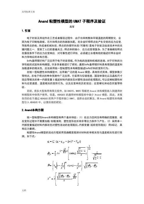
Anand 粘塑性模型的UMAT 子程序及验证高军1.引言电子封装及其组件在工艺或者服役过程中, 由于功率耗散和环境温度的周期变化, 会因为电子印制电路板、芯片和焊点的热膨胀失配,在合金钎焊焊点处产生交变的应力应变, 导致焊点的电、热或者机械失效。
焊点的热循环失效(可靠性)是电子封装及组装技术中的关键问题之一, 受到了人们的普遍关注。
焊点体积细小, 应力应变很复杂。
为了准确模拟焊点在服役条件下的应力应变响应, 对可靠性进行评估, 必须建立合理有效的描述钎焊合金材料力学响应的本构方程。
SnPb 基焊锡钎料广泛应用于电子封装领域,作为电的连接和机械的连接。
对于钎料的力学性能的试验和本构模型,许多学者都进行了研究。
通常SnPb 基焊锡钎料具有很强的温度和加载速率的相关性,应该采用统一型粘塑性本构模型描述SnPb 钎料的变形行为。
在统一型粘塑性本构模型中,应用最广泛的是Anand 模型。
具有形式简单,模型参数少等特点,在电子焊点的寿命预测中广泛应用。
它采用与位错密度、固溶体强化以及晶粒尺寸效应等相关的单一内部变量S 描述材料内部状态对塑性流动的宏观阻抗,可以反映粘塑性材料与应变速度、温度相关的变形行为,以及应变率的历史效应、应变硬化和动态回复等特征。
目前,很多大型商用有限元软件,如ANSYS 、MARC 等都把Anand 本构模型嵌入到通用材料模型库中供用户使用,但是,ABAQUS 的通用材料模型库中缺少Anand 模型。
因此,本报告目的在于通过ABAQUS 的用户子程序接口UMAT ,选择合适的算法,将Anand 粘塑性本构模型引入ABAQUS 中,以便后续的研究。
2.Anand 本构方程统一型粘塑性Anand 本构模型有两个基本特征:(1) 在应力空间没有明确的屈服面, 故在变形过程中不需要加载/卸载准则, 塑性变形在所有非零应力条件下产生。
(2) 采用单一内部变量描述材料内部状态对塑性流动的宏观阻抗。
1、为何需要使用用户材料子程序(User-Defined Material, UMAT )?很简单,当ABAQUS 没有提供我们需要的材料模型时。
所以,在决定自己定义一种新的材料模型之前,最好对ABAQUS 已经提供的模型心中有数,并且尽量使用现有的模型,因为这些模型已经经过详细的验证,并被广泛接受。
UMAT 子程序具有强大的功能,使用UMAT 子程序:(1)可以定义材料的本构关系,使用ABAQUS 材料库中没有包含的材料进行计算,扩充程序功能。
(2) 几乎可以用于力学行为分析的任何分析过程,几乎可以把用户材料属性赋予ABAQU S 中的任何单元。
(3) 必须在UMAT 中提供材料本构模型的雅可比(Jacobian )矩阵,即应力增量对应变增量的变化率。
(4) 可以和用户子程序“USDFLD ”联合使用,通过“USDFLD ”重新定义单元每一物质点上传递到UMAT 中场变量的数值。
2、需要哪些基础知识?先看一下ABAQUS 手册(ABAQUS Analysis User's Manual )里的一段话:Warning: The use of this option generally requires considerable expertise(一定的专业知识). The user is cautioned that the implementation (实现) of any realistic constitutive (基本) model requires extensive (广泛的) development and testing. Initial testing on a single eleme nt model with prescribed traction loading (指定拉伸载荷) is strongly recommended. 但这并不意味着非力学专业,或者力学基础知识不很丰富者就只能望洋兴叹,因为我们的任务不是开发一套完整的有限元软件,而只是提供一个描述材料力学性能的本构方程(Constitutive equation )而已。


前言有限元法是工程中广泛使用的一种数值计算方法。
它是力学、计算方法和计算机技术相结合的产物。
在工程应用中,有限元法比其它数值分析方法更流行的一个重要原因在于:相对与其它数值分析方法,有限元法对边界的模拟更灵活,近似程度更高。
所以,伴随着有限元理论以及计算机技术的发展,大有限元软件的应用证变得越来越普及。
ABAQUS软件一直以非线性有限元分析软件而闻名,这也是它和ANSYS,Nastran等软件的区别所在。
非线性有限元分析的用处越来越大,因为在所用材料非常复杂很多情况下,用线性分析来近似已不再有效。
比方说,一个复合材料就不能用传统的线性分析软件包进行分析。
任何与时间有关联,有较大位移量的情况都不能用线性分析法来处理。
多年前,虽然非线性分析能更适合、更准确的处理问题,但是由于当时计算设备的能力不够强大、非线性分析软件包线性分析功能不够健全,所以通常采用线性处理的方法。
这种情况已经得到了极大的改善,计算设备的能力变得更加强大、类似ABAQUS这样的产品功能日臻完善,应用日益广泛。
非线性有限元分析在各个制造行业得到了广泛应用,有不少大型用户。
航空航天业一直是非线性有限元分析的大客户,一个重要原因是大量使用复合材料。
新一代波音 787客机将全部采用复合材料。
只有像 ABAQUS这样的软件,才能分析包括多个子系统的产品耐久性能。
在汽车业,用线性有限元分析来做四轮耐久性分析不可能得到足够准确的结果.分析汽车的整体和各个子系统的性能要求(如悬挂系统等)需要进行非线性分析。
在土木工程业, ABAQUS能处理包括混凝土静动力开裂分析以及沥青混凝土方面的静动力分析,还能处理高度复杂非线性材料的损伤和断裂问题,这对于大型桥梁结构,高层建筑的结构分析非常有效。
瞬态、大变形、高级材料的碰撞问题必须用非线性有限元分析来计算。
线性分析在这种情况下是不适用的。
以往有一些专门的软件来分析碰撞问题,但现在ABAQUS在通用有限元软件包就能解决这些问题。

各个楼层及内容索引2-------------------------------------什么是UMAT3-------------------------------------UMAT功能简介4-------------------------------------UMAT开始的变量声明5-------------------------------------UMAT中各个变量的详细解释6-------------------------------------关于沙漏和横向剪切刚度7-------------------------------------UMAT流程和参数表格实例展示8-------------------------------------FORTRAN语言中的接口程序Interface9-------------------------------------关于UMAT是否可以用Fortran90编写的问题10-17--------------------------------Fortran77的一些有用的知识简介20-25\30-32-----------------------弹塑性力学相关知识简介34-37--------------------------------用户材料子程序实例JOhn-cook模型压缩包下载38-------------------------------------JOhn-cook模型本构简介图40-------------------------------------用户材料子程序实例JOhn-cook模型完整程序+david详细注解[欢迎大家来看看,并提供意见,完全是自己的diy的,不保证完全正确,希望共同探讨,以便更正,带"?"部分,还望各位大师\同仁指教]1 什么是UMAT???1.1 UMAT功能简介!!
前言有限元法是工程中广泛使用的一种数值计算方法。
它是力学、计算方法和计算机技术相结合的产物。
在工程应用中,有限元法比其它数值分析方法更流行的一个重要原因在于:相对与其它数值分析方法,有限元法对边界的模拟更灵活,近似程度更高。
所以,伴随着有限元理论以及计算机技术的发展,大有限元软件的应用证变得越来越普及。
ABAQUS软件一直以非线性有限元分析软件而闻名,这也是它和ANSYS,Nastran等软件的区别所在。
非线性有限元分析的用处越来越大,因为在所用材料非常复杂很多情况下,用线性分析来近似已不再有效。
比方说,一个复合材料就不能用传统的线性分析软件包进行分析。
任何与时间有关联,有较大位移量的情况都不能用线性分析法来处理。
多年前,虽然非线性分析能更适合、更准确的处理问题,但是由于当时计算设备的能力不够强大、非线性分析软件包线性分析功能不够健全,所以通常采用线性处理的方法。
这种情况已经得到了极大的改善,计算设备的能力变得更加强大、类似ABAQUS这样的产品功能日臻完善,应用日益广泛。
非线性有限元分析在各个制造行业得到了广泛应用,有不少大型用户。
航空航天业一直是非线性有限元分析的大客户,一个重要原因是大量使用复合材料。
新一代波音787客机将全部采用复合材料。
只有像 ABAQUS这样的软件,才能分析包括多个子系统的产品耐久性能。
在汽车业,用线性有限元分析来做四轮耐久性分析不可能得到足够准确的结果。
分析汽车的整体和各个子系统的性能要求(如悬挂系统等)需要进行非线性分析。
在土木工程业,ABAQUS能处理包括混凝土静动力开裂分析以及沥青混凝土方面的静动力分析,还能处理高度复杂非线性材料的损伤和断裂问题,这对于大型桥梁结构,高层建筑的结构分析非常有效。
瞬态、大变形、高级材料的碰撞问题必须用非线性有限元分析来计算。
线性分析在这种情况下是不适用的。
以往有一些专门的软件来分析碰撞问题,但现在ABAQUS在通用有限元软件包就能解决这些问题。
Anand 粘塑性模型的UMAT 子程序及验证高军1.引言电子封装及其组件在工艺或者服役过程中, 由于功率耗散和环境温度的周期变化, 会因为电子印制电路板、芯片和焊点的热膨胀失配,在合金钎焊焊点处产生交变的应力应变, 导致焊点的电、热或者机械失效。
焊点的热循环失效(可靠性)是电子封装及组装技术中的关键问题之一, 受到了人们的普遍关注。
焊点体积细小, 应力应变很复杂。
为了准确模拟焊点在服役条件下的应力应变响应, 对可靠性进行评估, 必须建立合理有效的描述钎焊合金材料力学响应的本构方程。
SnPb 基焊锡钎料广泛应用于电子封装领域,作为电的连接和机械的连接。
对于钎料的力学性能的试验和本构模型,许多学者都进行了研究。
通常SnPb 基焊锡钎料具有很强的温度和加载速率的相关性,应该采用统一型粘塑性本构模型描述SnPb 钎料的变形行为。
在统一型粘塑性本构模型中,应用最广泛的是Anand 模型。
具有形式简单,模型参数少等特点,在电子焊点的寿命预测中广泛应用。
它采用与位错密度、固溶体强化以及晶粒尺寸效应等相关的单一内部变量S 描述材料内部状态对塑性流动的宏观阻抗,可以反映粘塑性材料与应变速度、温度相关的变形行为,以及应变率的历史效应、应变硬化和动态回复等特征。
目前,很多大型商用有限元软件,如ANSYS 、MARC 等都把Anand 本构模型嵌入到通用材料模型库中供用户使用,但是,ABAQUS 的通用材料模型库中缺少Anand 模型。
因此,本报告目的在于通过ABAQUS 的用户子程序接口UMAT ,选择合适的算法,将Anand 粘塑性本构模型引入ABAQUS 中,以便后续的研究。
2.Anand 本构方程统一型粘塑性Anand 本构模型有两个基本特征:(1) 在应力空间没有明确的屈服面, 故在变形过程中不需要加载/卸载准则, 塑性变形在所有非零应力条件下产生。
(2) 采用单一内部变量描述材料内部状态对塑性流动的宏观阻抗。
一起学习UMAT的一些公式注释ZHANG chunyuherrliubs comments in formulas知识积累和储备在进行ABAQUS子程序UMAT的编写前,要弄清楚:ABAQUS调用UMAT子程序流程;要建立的材料模型的本构关系和屈服准则等;UMAT子程序中相关参数、以及矩阵的表达。
主要求解过程:每一个增量步开始,ABAQUS主程序在单元积分点上调用UMAT 子程序,并转入应变增量、时间步长及荷载增量,同时也传入当前已知的状态的应力、应变及其他求解过程相关的变量;UMAT子程序根据本构方程求解应力增量及其他相关的变量,提供Jacobian矩阵给ABAQUS主程序以形成整体刚度矩阵;主程序结合当前荷载增量求解位移增量,继而进行平衡校核;如果不满足指定的误差,ABAQUS将进行迭代直到收敛,然后进行下一增量步的求解。
弹性力学相关知识(基本)仿真论坛(/forum.php ... &highlight=UMAT)ABAQUS二次开发版块这个人帖子结合例子,列出了弹性力学的基本公式。
UMAT变量含义UMAT中可以得到的量增量步开始时刻的,应力(Stress),应变(Strain), 状态变量(Solution-dependent state variables (SDVs))增量步开始时刻的,应变增量(Strain increment),转角增量(Rotation increment),变形梯度(Deformation gradient)时间总值及增量(Total and incremental values of time),温度(Temperature),用户定义场变量材料常数,材料点的位置,特征单元长度当前分析步,增量步必须定义的变量应力,状态变量,材料Jacobian矩阵(本构关系)可以定义的变量应变能,塑性耗能,蠕变耗能新建议的时间增量变量分类UMAT中可以直接调用(Call ……)的子程序或子函数SINV(STRESS,SINV1,SINV2,NDI,NSHR)——用于计算应力不变量。
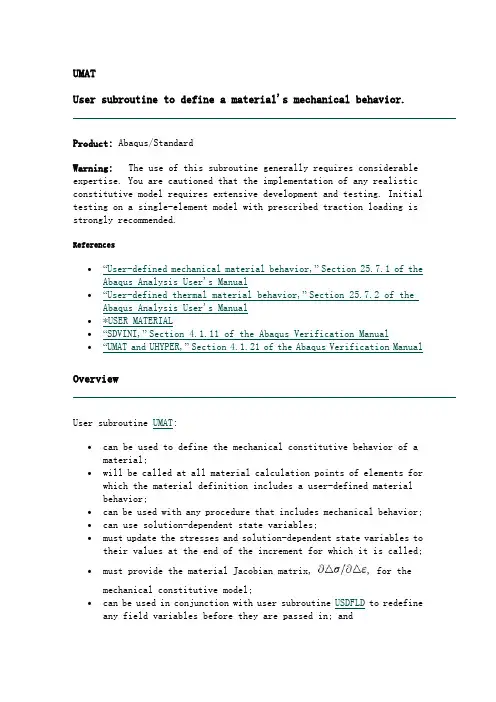
UMATUser subroutine to define a material's mechanical behavior.Product: Abaqus/StandardWarning: The use of this subroutine generally requires considerable expertise. You are cautioned that the implementation of any realistic constitutive model requires extensive development and testing. Initial testing on a single-element model with prescribed traction loading is strongly recommended.References∙“User-defined mechanical material behavior,” Section 25.7.1 of the Abaqus Analysis User's Manual∙“User-defined thermal material behavior,” Section 25.7.2 of the Abaqus Analysis User's Manual∙*USER MATERIAL∙“SDVINI,” Section 4.1.11 of the Abaqus Verification Manual∙“UMAT and UHYPER,” Section 4.1.21 of the Abaqus Verification Manual OverviewUser subroutine UMAT:∙can be used to define the mechanical constitutive behavior of a material;∙will be called at all material calculation points of elements for which the material definition includes a user-defined materialbehavior;∙can be used with any procedure that includes mechanical behavior;∙can use solution-dependent state variables;∙must update the stresses and solution-dependent state variables to their values at the end of the increment for which it is called;∙must provide the material Jacobian matrix, , for the mechanical constitutive model;∙can be used in conjunction with user subroutine USDFLD to redefine any field variables before they are passed in; andis described further in “User-defined mechanical material behavior,” Section 25.7.1 of the Abaqus Analysis User's Manual. Storage of stress and strain componentsIn the stress and strain arrays and in the matrices DDSDDE, DDSDDT, and DRPLDE, direct components are stored first, followed by shear components. There are NDI direct and NSHR engineering shear components. The order of the components is defined in “Conventions,” Section 1.2.2 of the Abaqus Analysis User's Manual. Since the number of active stress and strain components varies between element types, the routine must be coded to provide for all element types with which it will be used.Defining local orientationsIf a local orientation (“Orientations,” Section 2.2.5 of the Abaqus Analysis User's Manual) is used at the same point as user subroutine UMAT, the stress and strain components will be in the local orientation; and, in the case of finite-strain analysis, the basis system in which stress and strain components are stored rotates with the material.StabilityYou should ensure that the integration scheme coded in this routine is stable—no direct provision is made to include a stability limit in the time stepping scheme based on the calculations in UMAT.Convergence rateDDSDDE and—for coupled temperature-displacement and coupledthermal-electrical-structural analyses—DDSDDT, DRPLDE, and DRPLDT must be defined accurately if rapid convergence of the overall Newton scheme is to be achieved. In most cases the accuracy of this definition is the most important factor governing the convergence rate. Since nonsymmetric equation solution is as much as four times as expensive as the corresponding symmetric system, if the constitutive Jacobian (DDSDDE) is only slightly nonsymmetric (for example, a frictional material with a small frictionangle), it may be less expensive computationally to use a symmetric approximation and accept a slower convergence rate.An incorrect definition of the material Jacobian affects only the convergence rate; the results (if obtained) are unaffected.Special considerations for various element typesThere are several special considerations that need to be noted. Availability of deformation gradientThe deformation gradient is available for solid (continuum) elements, membranes, and finite-strain shells (S3/S3R, S4, S4R, SAXs, and SAXAs). It is not available for beams or small-strain shells. It is stored as a3 × 3 matrix with component equivalence DFGRD0(I,J) . For fully integrated first-order isoparametric elements (4-node quadrilaterals in two dimensions and 8-node hexahedra in three dimensions) the selectively reduced integration technique is used (also known as the technique). Thus, a modified deformation gradientis passed into user subroutine UMAT. For more details, see “Solid isoparametric quadrilaterals and hexahedra,” Section 3.2.4 of the Abaqus Theory Manual.Beams and shells that calculate transverse shear energyIf user subroutine UMAT is used to describe the material of beams or shells that calculate transverse shear energy, you must specify the transverse shear stiffness as part of the beam or shell section definition to define the transverse shear behavior. See “Shell section behavior,” Section 28.6.4 of the Abaqus Analysis User's Manual, and “Choosing a beam element,” Section 28.3.3 of the Abaqus Analysis User's Manual, for information on specifying this stiffness.Open-section beam elementsWhen user subroutine UMAT is used to describe the material response of beams with open sections (for example, an I-section), the torsional stiffness is obtained aswhere J is the torsional constant, A is the section area, k is a shear factor, and is the user-specified transverse shear stiffness (see “Transverse shear stiffness definition” in “Choosing a beam element,” Section 28.3.3 of the Abaqus Analysis User's Manual).Elements with hourglassing modesIf this capability is used to describe the material of elements with hourglassing modes, you must define the hourglass stiffness factor for hourglass control based on the total stiffness approach as part of the element section definition. The hourglass stiffness factor is not required for enhanced hourglass control, but you can define a scaling factor for the stiffness associated with the drill degree of freedom (rotation about the surface normal). See “Section controls,” Section 26.1.4 of the Abaqus Analysis User's Manual, for information on specifying the stiffness factor.Pipe-soil interaction elementsThe constitutive behavior of the pipe-soil interaction elements (see “Pipe-soil interaction elements,” Section 31.12.1 of the Abaqus Analysis User's Manual) is defined by the force per unit length caused by relative displacement between two edges of the element. The relative-displacements are available as “strains” (STRAN and DSTRAN). The corresponding forces per unit length must be defined in the STRESS array. The Jacobian matrix defines the variation of force per unit length with respect to relative displacement.For two-dimensional elements two in-plane components of “stress” and “strain” exist (NTENS=NDI=2, and NSHR=0). For three-dimensional elements three components of “stress” and “strain” exist (NTENS=NDI=3, and NSHR=0).Large volume changes with geometric nonlinearityIf the material model allows large volume changes and geometric nonlinearity is considered, the exact definition of the consistent Jacobian should be used to ensure rapid convergence. These conditions are most commonly encountered when considering either large elastic strains or pressure-dependent plasticity. In the former case, total-form constitutive equations relating the Cauchy stress to the deformation gradient are commonly used; in the latter case, rate-form constitutive laws are generally used.For total-form constitutive laws, the exact consistent Jacobian is defined through the variation in Kirchhoff stress:Here, J is the determinant of the deformation gradient, is the Cauchy stress, is the virtual rate of deformation, and is the virtual spin tensor, defined asandFor rate-form constitutive laws, the exact consistent Jacobian is given byUse with incompressible elastic materialsFor user-defined incompressible elastic materials, user subroutine UHYPER should be used rather than user subroutine UMAT. In UMAT incompressible materials must be modeled via a penalty method; that is, you must ensure that a finite bulk modulus is used. The bulk modulus should be large enough to model incompressibility sufficiently but small enough to avoid loss of precision. As a general guideline, the bulk modulus should be about– times the shear modulus. The tangent bulk modulus can be calculated fromIf a hybrid element is used with user subroutine UMAT, Abaqus/Standard will replace the pressure stress calculated from your definition of STRESS with that derived from the Lagrange multiplier and will modify the Jacobian appropriately.For incompressible pressure-sensitive materials the element choice is particularly important when using user subroutine UMAT. In particular, first-order wedge elements should be avoided. For these elements the technique is not used to alter the deformation gradient that is passed into user subroutine UMAT, which increases the risk of volumetric locking.Increments for which only the Jacobian can be definedAbaqus/Standard passes zero strain increments into user subroutine UMAT to start the first increment of all the steps and all increments of steps for which you have suppressed extrapolation (see “Procedures: overview,” Section 6.1.1 of the Abaqus Analysis User's Manual). In this case you can define only the Jacobian (DDSDDE).Utility routinesSeveral utility routines may help in coding user subroutine UMAT. Their functions include determining stress invariants for a stress tensor and calculating principal values and directions for stress or strain tensors. These utility routines are discussed in detail in “Obtaining stress invariants, principal stress/strain values and directions, and rotating tensors in an Abaqus/Standard analysis,” Section 2.1.11.User subroutine interfaceSUBROUTINE UMAT(STRESS,STATEV,DDSDDE,SSE,SPD,SCD,1 RPL,DDSDDT,DRPLDE,DRPLDT,2 STRAN,DSTRAN,TIME,DTIME,TEMP,DTEMP,PREDEF,DPRED,CMNAME,3 NDI,NSHR,NTENS,NSTATV,PROPS,NPROPS,COORDS,DROT,PNEWDT,4 CELENT,DFGRD0,DFGRD1,NOEL,NPT,LAYER,KSPT,KSTEP,KINC)CINCLUDE 'ABA_PARAM.INC'CCHARACTER*80 CMNAMEDIMENSION STRESS(NTENS),STATEV(NSTATV),1 DDSDDE(NTENS,NTENS),DDSDDT(NTENS),DRPLDE(NTENS),2 STRAN(NTENS),DSTRAN(NTENS),TIME(2),PREDEF(1),DPRED(1),3 PROPS(NPROPS),COORDS(3),DROT(3,3),DFGRD0(3,3),DFGRD1(3,3)user coding to define DDSDDE, STRESS, STATEV, SSE, SPD, SCDand, if necessary, RPL, DDSDDT, DRPLDE, DRPLDT, PNEWDTRETURNENDVariables to be definedIn all situationsDDSDDE(NTENS,NTENS)Jacobian matrix of the constitutive model, , where are thestress increments and are the strain increments. DDSDDE(I,J) defines the change in the Ith stress component at the end of the time increment caused by an infinitesimal perturbation of the Jth component of the strain increment array. Unless you invoke the unsymmetric equation solution capability for the user-defined material, Abaqus/Standard will use only the symmetric part of DDSDDE. The symmetric part of the matrix is calculated by taking one half the sum of the matrix and its transpose.STRESS(NTENS)This array is passed in as the stress tensor at the beginning of the increment and must be updated in this routine to be the stress tensor at the end of the increment. If you specified initial stresses (“Initial conditions in Abaqus/Standard and Abaqus/Explicit,” Section 32.2.1 of the Abaqus Analysis User's Manual), this array will contain the initial stresses at the start of the analysis. The size of this array depends on the value of NTENS as defined below. In finite-strain problems the stress tensor has already been rotated to account for rigid body motion in theincrement before UMAT is called, so that only the corotational part of the stress integration should be done in UMAT. The measure of stress used is “true” (Cauchy) stress.STATEV(NSTATV)An array containing the solution-dependent state variables. These are passed in as the values at the beginning of the increment unless they are updated in user subroutines USDFLD or UEXPAN, in which case the updated values are passed in. In all cases STATEV must be returned as the values at the end of the increment. The size of the array is defined as described in “Allocating space” in “User subroutines: overview,” Section 17.1.1 of the Abaqus Analysis User's Manual.In finite-strain problems any vector-valued or tensor-valued state variables must be rotated to account for rigid body motion of the material, in addition to any update in the values associated with constitutive behavior. The rotation increment matrix, DROT, is provided for this purpose.SSE, SPD, SCDSpecific elastic strain energy, plastic dissipation, and “creep” dissipation, respectively. These are passed in as the values at the start of the increment and should be updated to the corresponding specific energy values at the end of the increment. They have no effect on the solution, except that they are used for energy output.Only in a fully coupled thermal-stress or a coupledthermal-electrical-structural analysisRPLVolumetric heat generation per unit time at the end of the increment caused by mechanical working of the material.DDSDDT(NTENS)Variation of the stress increments with respect to the temperature.DRPLDE(NTENS)Variation of RPL with respect to the strain increments.DRPLDTVariation of RPL with respect to the temperature.Only in a geostatic stress procedure or a coupled pore fluiddiffusion/stress analysis for pore pressure cohesive elementsRPLRPL is used to indicate whether or not a cohesive element is open to the tangential flow of pore fluid. Set RPL equal to 0 if there is no tangential flow; otherwise, assign a nonzero value to RPL if an element is open. Once opened, a cohesive element will remain open to the fluid flow.Variable that can be updatedPNEWDTRatio of suggested new time increment to the time increment being used (DTIME, see discussion later in this section). This variable allows you to provide input to the automatic time incrementation algorithms in Abaqus/Standard (if automatic time incrementation is chosen). For a quasi-static procedure the automatic time stepping that Abaqus/Standard uses, which is based on techniques for integrating standard creep laws (see “Quasi-static analysis,” Section 6.2.5 of the Abaqus Analysis User's Manual), cannot be controlled from within the UMAT subroutine.PNEWDT is set to a large value before each call to UMAT.If PNEWDT is redefined to be less than 1.0, Abaqus/Standard must abandon the time increment and attempt it again with a smaller time increment. The suggested new time increment provided to the automatic time integration algorithms is PNEWDT × DTIME, where t he PNEWDT used is the minimum value for all calls to user subroutines that allow redefinition of PNEWDT for this iteration.If PNEWDT is given a value that is greater than 1.0 for all calls to user subroutines for this iteration and the increment converges in this iteration, Abaqus/Standard may increase the time increment. The suggested new time increment provided to the automatic time integration algorithms is PNEWDT × DTIME, where the PNEWDT used is the minimum value for all calls to user subroutines for this iteration.If automatic time incrementation is not selected in the analysis procedure, values of PNEWDT that are greater than 1.0 will be ignored and values of PNEWDT that are less than 1.0 will cause the job to terminate.Variables passed in for informationSTRAN(NTENS)An array containing the total strains at the beginning of the increment. If thermal expansion is included in the same material definition, the strains passed into UMAT are the mechanical strains only (that is, the thermal strains computed based upon the thermal expansion coefficient have been subtracted from the total strains). These strains are available for output as the “elastic” strains.In finite-strain problems the strain components have been rotated to account for rigid body motion in the increment before UMAT is called and are approximations to logarithmic strain.DSTRAN(NTENS)Array of strain increments. If thermal expansion is included in the same material definition, these are the mechanical strain increments (the total strain increments minus the thermal strain increments).TIME(1)Value of step time at the beginning of the current increment.TIME(2)Value of total time at the beginning of the current increment.DTIMETime increment.TEMPTemperature at the start of the increment.DTEMPIncrement of temperature.PREDEFArray of interpolated values of predefined field variables at this point at the start of the increment, based on the values read in at the nodes.DPREDArray of increments of predefined field variables.CMNAMEUser-defined material name, left justified. Some internal material models are given names starting with the “ABQ_” character string. To avoid conflict, you should not use “ABQ_” as the leading string for CMNAME.NDINumber of direct stress components at this point.NSHRNumber of engineering shear stress components at this point.NTENSSize of the stress or strain component array (NDI + NSHR).NSTATVNumber of solution-dependent state variables that are associated with this material type (defined as described in “Allocating space” in “User subroutines: overview,” Section 17.1.1 of the Abaqus Analysis User's Manual).PROPS(NPROPS)User-specified array of material constants associated with this user material.NPROPSUser-defined number of material constants associated with this user material.COORDSAn array containing the coordinates of this point. These are the current coordinates if geometric nonlinearity is accounted for during the step (see “Procedures: overview,” Section 6.1.1 of the Abaqus Analysis User's Manual); otherwise, the array contains the original coordinates of the point.DROT(3,3)Rotation increment matrix. This matrix represents the increment of rigid body rotation of the basis system in which the components of stress (STRESS) and strain (STRAN) are stored. It is provided so that vector- ortensor-valued state variables can be rotated appropriately in this subroutine: stress and strain components are already rotated by this amount before UMAT is called. This matrix is passed in as a unit matrix for small-displacement analysis and for large-displacement analysis if the basis system for the material point rotates with the material (as in a shell element or when a local orientation is used).CELENTCharacteristic element length, which is a typical length of a line across an element for a first-order element; it is half of the same typical length for a second-order element. For beams and trusses it is a characteristic length along the element axis. For membranes and shells it is a characteristic length in the reference surface. For axisymmetric elementsit is a characteristic length in the plane only. For cohesive elementsit is equal to the constitutive thickness.DFGRD0(3,3)Array containing the deformation gradient at the beginning of the increment. If a local orientation is defined at the material point, the deformation gradient components are expressed in the local coordinate system defined by the orientation at the beginning of the increment. For a discussion regarding the availability of the deformation gradient for various element types, see “Availability of deformation gradient.”DFGRD1(3,3)Array containing the deformation gradient at the end of the increment. If a local orientation is defined at the material point, the deformation gradient components are expressed in the local coordinate system defined by the orientation. This array is set to the identity matrix if nonlinear geometric effects are not included in the step definition associated withthis increment. For a discussion regarding the availability of the deformation gradient for various element types, see “Availability of deformation gradient.”NOELElement number.NPTIntegration point number.LAYERLayer number (for composite shells and layered solids).KSPTSection point number within the current layer.KSTEPStep number.KINCIncrement number.Example: Using more than one user-defined mechanical material modelTo use more than one user-defined mechanical material model, the variable CMNAME can be tested for different material names inside user subroutine UMAT as illustrated below:IF (CMNAME(1:4) .EQ. 'MAT1') THENCALL UMAT_MAT1(argument_list)ELSE IF(CMNAME(1:4) .EQ. 'MAT2') THENCALL UMAT_MAT2(argument_list)END IFUMAT_MAT1 and UMAT_MAT2 are the actual user material subroutines containing the constitutive material models for each material MAT1 and MAT2, respectively. Subroutine UMAT merely acts as a directory here. The argument list may be the same as that used in subroutine UMAT.Example: Simple linear viscoelastic materialAs a simple example of the coding of user subroutine UMAT, consider the linear, viscoelastic model shown in Figure 1.1.40–1. Although this is not a very useful model for real materials, it serves to illustrate how to code the routine.Figure 1.1.40–1 Simple linear viscoelastic model.The behavior of the one-dimensional model shown in the figure iswhere and are the time rates of change of stress and strain. This can be generalized for small straining of an isotropic solid asandwhereand , , , , and are material constants ( and are the Lamé constants).A simple, stable integration operator for this equation is the central difference operator:where f is some function, is its value at the beginning of the increment,is the change in the function over the increment, and is the timeincrement.Applying this to the rate constitutive equations above givesandso that the Jacobian matrix has the termsandThe total change in specific energy in an increment for this material iswhile the change in specific elastic strain energy iswhere D is the elasticity matrix:No state variables are needed for this material, so the allocation of space for them is not necessary. In a more realistic case a set of parallel models of this type might be used, and the stress components in each model might be stored as state variables.For our simple case a user material definition can be used to read in the five constants in the order , , , , and so thatThe routine can then be coded as follows:SUBROUTINE UMAT(STRESS,STATEV,DDSDDE,SSE,SPD,SCD,1 RPL,DDSDDT,DRPLDE,DRPLDT,2 STRAN,DSTRAN,TIME,DTIME,TEMP,DTEMP,PREDEF,DPRED,CMNAME,3 NDI,NSHR,NTENS,NSTATV,PROPS,NPROPS,COORDS,DROT,PNEWDT,4 CELENT,DFGRD0,DFGRD1,NOEL,NPT,LAYER,KSPT,KSTEP,KINC)CINCLUDE 'ABA_PARAM.INC'CCHARACTER*80 CMNAMEDIMENSION STRESS(NTENS),STATEV(NSTATV),1 DDSDDE(NTENS,NTENS),2 DDSDDT(NTENS),DRPLDE(NTENS),3 STRAN(NTENS),DSTRAN(NTENS),TIME(2),PREDEF(1),DPRED(1),4 PROPS(NPROPS),COORDS(3),DROT(3,3),DFGRD0(3,3),DFGRD1(3,3) DIMENSION DSTRES(6),D(3,3)CC EVALUATE NEW STRESS TENSORCEV = 0.DEV = 0.DO K1=1,NDIEV = EV + STRAN(K1)DEV = DEV + DSTRAN(K1)END DOCTERM1 = .5*DTIME + PROPS(5)TERM1I = 1./TERM1TERM2 = (.5*DTIME*PROPS(1)+PROPS(3))*TERM1I*DEVTERM3 = (DTIME*PROPS(2)+2.*PROPS(4))*TERM1ICDO K1=1,NDIDSTRES(K1) = TERM2+TERM3*DSTRAN(K1)1 +DTIME*TERM1I*(PROPS(1)*EV2 +2.*PROPS(2)*STRAN(K1)-STRESS(K1))STRESS(K1) = STRESS(K1) + DSTRES(K1)END DOCTERM2 = (.5*DTIME*PROPS(2) + PROPS(4))*TERM1II1 = NDIDO K1=1,NSHRI1 = I1+1DSTRES(I1) = TERM2*DSTRAN(I1)+1 DTIME*TERM1I*(PROPS(2)*STRAN(I1)-STRESS(I1))STRESS(I1) = STRESS(I1)+DSTRES(I1)END DOCC CREATE NEW JACOBIANCTERM2 = (DTIME*(.5*PROPS(1)+PROPS(2))+PROPS(3)+1 2.*PROPS(4))*TERM1ITERM3 = (.5*DTIME*PROPS(1)+PROPS(3))*TERM1IDO K1=1,NTENSDO K2=1,NTENSDDSDDE(K2,K1) = 0.END DOEND DOCDO K1=1,NDIDDSDDE(K1,K1) = TERM2END DOCDO K1=2,NDIN2 = K1–1DO K2=1,N2DDSDDE(K2,K1) = TERM3DDSDDE(K1,K2) = TERM3END DOEND DOTERM2 = (.5*DTIME*PROPS(2)+PROPS(4))*TERM1II1 = NDIDO K1=1,NSHRI1 = I1+1DDSDDE(I1,I1) = TERM2END DOCC TOTAL CHANGE IN SPECIFIC ENERGYCTDE = 0.DO K1=1,NTENSTDE = TDE + (STRESS(K1)-.5*DSTRES(K1))*DSTRAN(K1) END DOCC CHANGE IN SPECIFIC ELASTIC STRAIN ENERGYCTERM1 = PROPS(1) + 2.*PROPS(2)DO K1=1,NDID(K1,K1) = TERM1END DODO K1=2,NDIN2 = K1-1DO K2=1,N2D(K1,K2) = PROPS(1)D(K2,K1) = PROPS(1)END DOEND DODEE = 0.DO K1=1,NDITERM1 = 0.TERM2 = 0.DO K2=1,NDITERM1 = TERM1 + D(K1,K2)*STRAN(K2)TERM2 = TERM2 + D(K1,K2)*DSTRAN(K2)END DODEE = DEE + (TERM1+.5*TERM2)*DSTRAN(K1)END DOI1 = NDIDO K1=1,NSHRI1 = I1+1DEE = DEE + PROPS(2)*(STRAN(I1)+.5*DSTRAN(I1))*DSTRAN(I1) END DOSSE = SSE + DEESCD = SCD + TDE – DEERETURNEND。

UMAT全过程-"技术篇"[写在前面:这篇文章是UMAT全过程-感想篇的姊妹篇,答应要给大家写的一篇帖子,同时也是为了记录自己的学习过程,与大家分享!首先指出,俺的"技术篇"--是加了引号的,因为确实称不上有多么大的技术含量,还望大家莫笑偶!只不过一是跟那个感想篇形成一个对照,同时主要内容为自己编子程序过程中涉及的技术边边上的小问题的一些解决方法,供仿友们参考!偶不是谦虚,也不是一个低调的人,大家谢谢和支持的话,我先行谢过啦!更希望大家能提出质疑或者别的更好的办法,大家相互交流,共同进步!]----------------------------------------------------------------------------*转*入*正*题*第一部分:相关知识[特别声明,这部分来自于华中科技大学杨曼娟同学的硕士学位论文,在此对作者表示感谢!--大家可以去知网下载]----------------------------------------------------------------------------1.ABAQUS中材料非线性问题的处理ABAQUS中材料非线性问题用Newton-Raphson法来求解。
首先将载荷分为若干个微小增量,结构受到一个微小增量△P。
ABAQUS用与初始结构位移相对应的初始刚度矩阵K0和荷载增量△P计算出结构的在这一步增量后的位移修正Ca、修正后的位移值Ua和相应的新的刚度矩阵Ka。
ABAQUS用新的刚度矩阵计算结构的内力Ia,荷载P和Ia的差值为迭代的残余力Ra,即Ra=P-Ia。
如果Ra在模型内的每个自由度上的值都为零,如图2-2中的a点,则结构处于平衡状态。
但在非线性问题中,通常Ra是不可能为零,ABAQUS为此设置了一个残余力容差。
如果Ra小于这个数字,ABAQUS就认为结构的内外力是平衡的。
一般这个缺省值取为平均内力的0.5%(如图2-2)。
SUBROUTINE UMAT(STRESS,STATEV,DDSDDE,SSE,SPD,SCD,1 RPL,DDSDDT,DRPLDE,DRPLDT,2 STRAN,DSTRAN,TIME,DTIME,TEMP,DTEMP,PREDEF,DPRED,CMNAME,3 NDI,NSHR,NTENS,NSTATV,PROPS,NPROPS,COORDS,DROT,PNEWDT,4 CELENT,DFGRD0,DFGRD1,NOEL,NPT,LAYER,KSPT,KSTEP,KINC)CINCLUDE 'ABA_PARAM.INC'CCHARACTER*80 CMNAMEDIMENSION STRESS(NTENS),STATEV(NSTATV),1 DDSDDE(NTENS,NTENS),2 DDSDDT(NTENS),DRPLDE(NTENS),3 STRAN(NTENS),DSTRAN(NTENS),TIME(2),PREDEF(1),DPRED(1),4 PROPS(NPROPS),COORDS(3),DROT(3,3),DFGRD0(3,3),DFGRD1(3,3)CDIMENSION STRANT(6),CFULL(6,6),CDFULL(6,6),DCDDFV(6,6),1 DCDDMV(6,6),DCDDDV(6,6),DFFDE(6),DFMDE(6),DFDDE(6),2 TEMP1(6),TEMP2(6),TEMP3(6),TEMP4(6),TEMP5(6),TEMP6(6),3 TEMP7(6,6)PARAMETER (ZERO = 0.D0,ONE = 1.D0,TWO = 2.D0,THREE = 3.D0)C 输入材料弹性参数e1=props(1)e2=props(2)e3=props(3)u12=props(4)u13=props(5)u23=props(6)g12=props(7)g13=props(8)g23=props(9)C 输入材料的强度参数,用于失效判断。
⼦程序(UMAT)基本操作过程1UMAT操作过程操作过程:1、CAE建模、定义边界条件、载荷条件2、定义UMATProperty>General>User materialMechanical Constants 中为⽤户输⼊到⼦程序中的参数。
这时只能在General栏中定义参数,如密度等,这时不能再在Mechanical中定义杨⽒模量等,此时杨⽒模量、泊松⽐等数就需要在Mechanical Constants中输⼊到⼦程序中。
定义剪切刚度Model>Edit Keywords 中直接输⼊到inp⽂件中。
“*Shell Section”后⾯添加*Transverse Shear5.31e8,5.31e8,0在定义剪切刚度时⼀定要注意,⼀定要按帮助⽂档中公式计算⽽得并不是任意取值。
对于正交各项异性壳单元其中t为层合板厚度。
Depvar 中的数字与Mechanical Constants栏中定义的参数数量相等。
3编辑.for后缀的⼦程序3.1 推导出本构关系建⽴刚度矩阵时最好是直接指定刚度阵的每⼀项的⽅法得到刚度阵。
3.2更新应⼒下⾯是各项同性弹性本构关系(刚度阵)及应⼒更新。
DO K1=1,NTENSDO K2=1,NTENSDDSDDE(K1,K2)=ZEROEND DOEND DODO K1=1,NDIDO K2=1,NDIDDSDDE(K2,K1)=EBULK3END DOEND DODO K1=1,NDIDO K2=1,NDIDDSDDE(K1,K1)=EG2END DOEND DODO K1=NDI+1,NTENSDDSDDE(K1,K1)=EG3END DODO K1=1,NTENSDO K2=1,NTENSSTRESS(K1)=STRESS(K1)+DDSDDE(K1,K2)*DSTRAN(K2)END DOEND DO注意:UMAT⼦程序中并不是⼀定要写成增量形式,建⽴Jacobian矩阵,只要能做到更新应⼒即可,写成全量形式也可以。
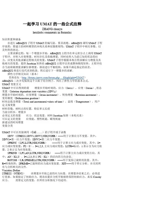
Anand粘塑性模型的UMAT子程序及验证高军1.引言电子封装及其组件在工艺或者服役过程中, 由于功率耗散和环境温度的周期变化, 会因为电子印制电路板、芯片和焊点的热膨胀失配,在合金钎焊焊点处产生交变的应力应变, 导致焊点的电、热或者机械失效。
焊点的热循环失效(可靠性)是电子封装及组装技术中的关键问题之一, 受到了人们的普遍关注。
焊点体积细小, 应力应变很复杂。
为了准确模拟焊点在服役条件下的应力应变响应, 对可靠性进行评估, 必须建立合理有效的描述钎焊合金材料力学响应的本构方程。
SnPb基焊锡钎料广泛应用于电子封装领域,作为电的连接和机械的连接。
对于钎料的力学性能的试验和本构模型,许多学者都进行了研究。
通常SnPb基焊锡钎料具有很强的温度和加载速率的相关性,应该采用统一型粘塑性本构模型描述SnPb钎料的变形行为。
在统一型粘塑性本构模型中,应用最广泛的是Anand模型。
具有形式简单,模型参数少等特点,在电子焊点的寿命预测中广泛应用。
它采用与位错密度、固溶体强化以及晶粒尺寸效应等相关的单一内部变量S描述材料内部状态对塑性流动的宏观阻抗,可以反映粘塑性材料与应变速度、温度相关的变形行为,以及应变率的历史效应、应变硬化和动态回复等特征。
目前,很多大型商用有限元软件,如ANSYS、MARC等都把Anand本构模型嵌入到通用材料模型库中供用户使用,但是,ABAQUS的通用材料模型库中缺少Anand模型。
因此,本报告目的在于通过ABAQUS的用户子程序接口UMAT,选择合适的算法,将Anand粘塑性本构模型引入ABAQUS中,以便后续的研究。
2.Anand本构方程统一型粘塑性Anand本构模型有两个基本特征:(1) 在应力空间没有明确的屈服面, 故在变形过程中不需要加载/卸载准则, 塑性变形在所有非零应力条件下产生。
(2) 采用单一内部变量描述材料内部状态对塑性流动的宏观阻抗。
内部变量(或称变形阻抗) 用S标记, 具有应力量纲。
UMAT以及depvar整理by warmwormdk最近一直在论坛查资料,对自己感兴趣的一些问题专门进行了整理,希望对大家有所帮助,也希望能获得小小的奖励啊,哈哈1 UMAT的状态变量问题Q:用DEPVAR定义的状态变量个数假设为10个。
是不是说一个积分点的状态变量是10个,单元的积分点是4的话,那么单元的状态变量就是40个。
也就是自己要存储单元变量的话,就得按40个状态变量来。
是不是呢?A:有人说跟我说,DEPVAR定义的状态变量个数指每个积分点的状态变量个数。
abaqus会自动为每个单元的每个积分点开辟这样大小的状态变量数组,abaqus调用umat时能够自动根据单元好和积分点向umat提供状态变量,在此基础上umat修改状态变量。
2 umat里的STATEV变量怎么输出到odb文件中Q:比如我想知道statev(10)的odb文件,怎么输出?又怎么打开.statev(10)是我自己定义的damage变量,请各位赐教A 在element关键词中添加SDV,就像下面这样。
*Element Output, directions=YESALPHA, LE, PE, PEEQ, PEMAG, PS, S, STH,SE, SF, VE, VEEQ, VS, SDV3Q statev(?)请问这个状态变量()内的数字代表什么含义?对应的变量是不是固定的?各自对应着哪些变量?A:括号中的数代表这个变量矩阵的维数,这个值等于depvar的值。
4 umat中DEPVAR有几种定义方式?Q;UMAT中状态变量的定义方式,一般有两种形式,一是在inp文件中采用*initial conditions定义,二是特殊情况下可以采用SDVINI来定义; 目前的疑问是,是否还有其他定义状态变量的方式? 请专家针对上传的附件给于指点多谢! 附件中的例子来自ABAQUS HELP中的例子! 请问例子中INP文件中是如何定义状态变量的 THANKSA:初值可以采用SDVINI来定义程序运行中用以下代码更新DO 310 K1=1,NTENSSTATEV(K1)=EELAS(K1)STATEV(K1+NTENS)=EPLAS(K1)310 CONTINUESTATEV(1+2*NTENS)=EQPLASCRETURNEND5 umat子程序定义问题?Q: 在umat中定义的参数在材料中需不需再定义了?比如我umat 中已经给了密度了。
APPENDIXNeo-Hookean Hyperelatic Material User SubroutineThis program is based on the derivation of hyperelastic material constitutive model inSection . A stress and strain relationship was derived from the neo-Hookean hyperelastic material constitutive model that is normally represented as the strain energywith strain invariants.subroutine vumatC Read only unmodifiablevariables -1 nblock, ndir, nshr, nstatev, nfieldv, nprops, lanneal,2 stepTime, totalTime, dt, cmname, coordMp, charLength,3 props, density, strainInc, relSpinInc,4 tempOld, stretchOld, defgradOld, fieldOld,5 stressOld, stateOld, enerInternOld, enerInelasOld,6 tempNew, stretchNew, defgradNew, fieldNew,C Write only modifiable variables -7 stressNew, stateNew, enerInternNew, enerInelasNewCinclude ''Cdimension propsnprops, densitynblock, coordMpnblock,,1 charLengthnblock, strainIncnblock,ndir+nshr,2 relSpinIncnblock,nshr, tempOldnblock,3 stretchOldnblock,ndir+nshr,4 defgradOldnblock,ndir+nshr+nshr,5 fieldOldnblock,nfieldv, stressOldnblock,ndir+nshr,6 stateOldnblock,nstatev, enerInternOldnblock,7 enerInelasOldnblock, tempNewnblock,8 stretchNewnblock,ndir+nshr,8 defgradNewnblock,ndir+nshr+nshr,9 fieldNewnblock,nfieldv,1 stressNewnblock,ndir+nshr, stateNewnblock,nstatev,2 enerInternNewnblock, enerInelasNewnblockCcharacter80 cmnameCif cmname1:6 .eq. 'VUMAT0' thencall VUMAT0nblock, ndir, nshr, nstatev, nfieldv, nprops, lanneal,2 stepTime, totalTime, dt, cmname, coordMp, charLength,3 props, density, strainInc, relSpinInc,4 tempOld, stretchOld, defgradOld, fieldOld,5 stressOld, stateOld, enerInternOld, enerInelasOld,6 tempNew, stretchNew, defgradNew, fieldNew,117else if cmname1:6 .eq. 'VUMAT1' thencall VUMAT1nblock, ndir, nshr, nstatev, nfieldv, nprops, lanneal,2 stepTime, totalTime, dt, cmname, coordMp, charLength,3 props, density, strainInc, relSpinInc,4 tempOld, stretchOld, defgradOld, fieldOld,5 stressOld, stateOld, enerInternOld, enerInelasOld,6 tempNew, stretchNew, defgradNew, fieldNew,7 stressNew, stateNew, enerInternNew, enerInelasNewend ifendCsubroutine vumat0C Read only -nblock, ndir, nshr, nstatev, nfieldv, nprops, lanneal, stepTime, totalTime, dt, cmname, coordMp, charLength, props, density, strainInc, relSpinInc,tempOld, stretchOld, defgradOld, fieldOld,stressOld, stateOld, enerInternOld, enerInelasOld, tempNew, stretchNew, defgradNew, fieldNew,C Write only -Cinclude ''Cdimension coordMpnblock,, charLengthnblock, propsnprops,1 densitynblock, strainIncnblock,ndir+nshr,2 relSpinIncnblock,nshr, tempOldnblock,3 stretchOldnblock,ndir+nshr,4 defgradOldnblock,ndir+nshr+nshr,5 fieldOldnblock,nfieldv, stressOldnblock,ndir+nshr,6 stateOldnblock,nstatev, enerInternOldnblock,7 enerInelasOldnblock, tempNewnblock,8 stretchNewnblock,ndir+nshr,9 defgradNewnblock,ndir+nshr+nshr,1 fieldNewnblock,nfieldv,2 stressNewnblock,ndir+nshr, stateNewnblock,nstatev,3 enerInternNewnblock, enerInelasNewnblockCdimension devianblock,ndir+nshr,1 BBarnblock,4, stretchNewBarnblock,4, intv2Ccharacter80 cmnameparameter zero = , one = , two = , three = ,four = , half =real C10,D1,ak,twomu,amu,alamda,hydro,vonMises, maxShear,1 midStrain, maxPrincipalStrain118Cintv1 = ndirintv2 = nshrCif ndir .ne. 3 .or. nshr .ne. 1 thencall xplb_abqerr1,'Subroutine VUMAT is implemented 'Q. zero then do k=1,nblocktrace1 = strainInck,1 + strainInck,2 + strainInck,3 stressNewk,1 = stressOldk,1+ twomu strainInck,1 + alamda trace1stressNewk,2 = stressOldk,2+ twomu strainInck,2 + alamda trace1stressNewk,3 = stressOldk,3+ twomu strainInck,3 + alamda trace1stressNewk,4 = stressOldk,4+ twomu strainInck,4C write6, totalTime,k,defgradNewk, 1,stretchNewk,1,C 1 stressNewk,2,stressNewk,3,stressNewk,4end doelsedo k=1,nblockCC JACOBIAN OF STRETCH TENSOR U is symmetric and in local axisCdet=stretchNewk, 31191 stretchNewk, 1stretchNewk, 2-stretchNewk, 4twoscale=det-ONE/THREEstretchNewBark, 1=stretchNewk, 1scale stretchNewBark, 2=stretchNewk, 2scale stretchNewBark, 3=stretchNewk, 3scale stretchNewBark, 4=stretchNewk, 4scaleCC CALCULATE LEFT CAUCHY-GREEN TENSOR B is symmetricCBBark,1=stretchNewBark, 1two+stretchNewBark, 4two BBark,2=stretchNewBark, 2two+stretchNewBark, 4twoBBark,3=stretchNewBark, 3twoBBark,4=stretchNewBark, 1stretchNewBark, 4 + 1 stretchNewBark, 2stretchNewBark, 4CC CALCULATE STRESS tensorCTRBBar=BBark,1+BBark,2+BBark,3EG=twoC10/detPR=two/D1det-onestressNewk,1=EGBBark,1-TRBBar/Three + PR stressNewk,2=EGBBark,2-TRBBar/Three + PR stressNewk,3=EGBBark,3-TRBBar/Three + PR stressNewk,4=EG BBark,4CC Update the specific internal energyCstressPower = half1 stressOldk,1+stressNewk,1 strainInck,1 +2 stressOldk,2+stressNewk,2 strainInck,2 +3 stressOldk,3+stressNewk,3 strainInck,3 +4 stressOldk,4+stressNewk,4 strainInck,4 enerInternNewk = enerInternOldk1 + stressPower / densitykCC Strains under corotational coordinates CstateNewk,1 = stateOldk,1 + strainInck,1 stateNewk,2 = stateOldk,2 + strainInck,2 stateNewk,3 = stateOldk,3 + strainInck,3 stateNewk,4 = stateOldk,4 + strainInck,4 CC Calculate vonMisesChydro = stressNewk,1+stressNewk,2+ 1201 stressNewk,3/3.do k1=1,ndirdeviak,k1 = stressNewk,k1 - hydroend dodo k1=ndir+1,ndir+nshrdeviak,k1 = stressNewk,k1end dovonMises = 0.do k1=1,ndirvonMises = vonMises + deviak,k12end dodo k1=ndir+1,ndir+nshrvonMises = vonMises + 2deviak,k12end dovonMises = sqrt3./2vonMisesC use 3/2 will get 2 intCC write6, totalTime,defgradNewk, 4,stretchNewk,4C 1 ,defgradNewk,3,defgradNewk,4,defgradNewk,5C ,det,TRBBarC 1 ,stressNewk,1,stressNewk,2,stressNewk,3,stressNewk,4 CC Failure CriteriaCmidStrain = stateNewk,1 + stateNewk,2maxShear = sqrtstateNewk,1 - midStrain2. +1 stateNewk,42.if midStrain .GE. 0. thenmaxPrincipalStrain = midStrain + maxShearelsemaxPrincipalStrain = maxShear - midStrainend ifif vonMises .GE. thenstateNewk,5 = 0end ifend doend ifreturnendCsubroutine vumat1C Read only -nblock, ndir, nshr, nstatev, nfieldv, nprops, lanneal, stepTime, totalTime, dt, cmname, coordMp, charLength, props, density, strainInc, relSpinInc,tempOld, stretchOld, defgradOld, fieldOld,121stressOld, stateOld, enerInternOld, enerInelasOld, tempNew, stretchNew, defgradNew, fieldNew,C Write only -stressNew, stateNew, enerInternNew, enerInelasNewCinclude ''dimension coordMpnblock,, charLengthnblock, propsnprops,1 densitynblock, strainIncnblock,ndir+nshr,2 relSpinIncnblock,nshr, tempOldnblock,3 stretchOldnblock,ndir+nshr,4 defgradOldnblock,ndir+nshr+nshr,5 fieldOldnblock,nfieldv, stressOldnblock,ndir+nshr,6 stateOldnblock,nstatev, enerInternOldnblock,7 enerInelasOldnblock, tempNewnblock,8 stretchNewnblock,ndir+nshr,9 defgradNewnblock,ndir+nshr+nshr,1 fieldNewnblock,nfieldv,2 stressNewnblock,ndir+nshr, stateNewnblock,nstatev,3 enerInternNewnblock, enerInelasNewnblockCdimension devianblock,ndir+nshr,1 BBarnblock,4, stretchNewBarnblock,4, intv2Ccharacter80 cmnameparameter zero = , one = , two = , three = ,four = , half =real C10,D1,ak,twomu,amu,alamda,hydro,vonMisesCintv1 = ndirintv2 = nshrCif ndir .ne. 3 .or. nshr .ne. 1 thencall xplb_abqerr1,'Subroutine VUMAT is implemented 'Q. zero then do k=1,nblocktrace1 = strainInck,1 + strainInck,2 + strainInck,3 stressNewk,1 = stressOldk,1+ twomu strainInck,1 + alamda trace1stressNewk,2 = stressOldk,2+ twomu strainInck,2 + alamda trace1stressNewk,3 = stressOldk,3+ twomu strainInck,3 + alamda trace1stressNewk,4 = stressOldk,4+ twomu strainInck,4C write6, totalTime,k,defgradNewk, 1,stretchNewk,1,C 1 stressNewk,2,stressNewk,3,stressNewk,4end doelsedo k=1,nblockCC JACOBIAN OF STRETCH TENSOR U is symmetric and in localCdet=stretchNewk, 31 stretchNewk, 1stretchNewk, 2-stretchNewk, 4two scale=det-ONE/THREEstretchNewBark, 1=stretchNewk, 1scale stretchNewBark, 2=stretchNewk, 2scale stretchNewBark, 3=stretchNewk, 3scale stretchNewBark, 4=stretchNewk, 4scaleCC CALCULATE LEFT CAUCHY-GREEN TENSOR B is symmetricCBBark,1=stretchNewBark, 1two+stretchNewBark, 4two BBark,2=stretchNewBark, 2two+stretchNewBark, 4two BBark,3=stretchNewBark, 3twoBBark,4=stretchNewBark, 1stretchNewBark, 4 +1 stretchNewBark, 2stretchNewBark, 4CC CALCULATE STRESS tensorCTRBBar=BBark,1+BBark,2+BBark,3EG=twoC10/detPR=two/D1det-onestressNewk,1=EGBBark,1-TRBBar/Three + PR stressNewk,2=EGBBark,2-TRBBar/Three + PR stressNewk,3=EGBBark,3-TRBBar/Three + PR stressNewk,4=EG BBark,4CC Update the specific internal energyCstressPower = half1 stressOldk,1+stressNewk,1 strainInck,1 +2 stressOldk,2+stressNewk,2 strainInck,2 +3 stressOldk,3+stressNewk,3 strainInck,3 +4 stressOldk,4+stressNewk,4 strainInck,4 enerInternNewk = enerInternOldk1 + stressPower / densitykCC Strains under corotational coordinatesCstateNewk,1 = stateOldk,1 + strainInck,1 stateNewk,2 = stateOldk,2 + strainInck,2stateNewk,3 = stateOldk,3 + strainInck,3 stateNewk,4 = stateOldk,4 + strainInck,4CC Calculate vonMisesChydro = stressNewk,1+stressNewk,2+1 stressNewk,3/3.do k1=1,ndirdeviak,k1 = stressNewk,k1 - hydroend dodo k1=ndir+1,ndir+nshrdeviak,k1 = stressNewk,k1end dovonMises = 0.do k1=1,ndirvonMises = vonMises + deviak,k12end dodo k1=ndir+1,ndir+nshrvonMises = vonMises + 2deviak,k12end dovonMises = sqrt3./2vonMisesC write6, totalTime,defgradNewk, 4,stretchNewk,4C 1 ,defgradNewk,3,defgradNewk,4,defgradNewk,5C ,det,TRBBarC 1 ,stressNewk,1,stressNewk,2,stressNewk,3,stressNewk,4 124end doend ifreturnend。
UMAT全过程——技术篇 1.ABAQUS中非线性问题的处理2.用户子程序接口3.用户子程序和主程序的结合4.用户材料子程序UMAT接口的原理5.UMAT子程序流程ABAQUS是怎么计算的
I.ABAQUS一共有42个用户子程序接口,15个应用程序接口,可以定义包括边界条
件,荷载条件,接触条件,材料特性以及利用用户子程序和其它应用软件进行数值交换。
1.根据ABAQUS提供的相应接口,按照FORTRAN语法自己编写的代码,是一个独立的程序单元,可以独立地被储存和编译,也能被其他程序单元引用。
I.一般结构形式
II.
一个算例中,可以用到多个用户子程序,但必须把它们放在一个以.for为扩展名的文件中。
III.运行带有用户子程序的算例的两种方法
1.在CAE中运行,在EDIT JOB菜单中的GENRAL子菜单的USERSUBROUTINE GILE对话框中选择用户子程序所在的文件
2.在MAND中运行语法如下
IV.编制用户子程序时应注意:
1.用户子程序相互之间不能调用,可以调用用户自己编写的Fortran子程序和
ABAQUS应用程序,ABAQUS应用程序必须由用户子程序调用。
编写Fortran子程序时,建议子程序以K开头,以免和ABAQUS内部程序冲突。
2.用户在用户子程序中利用OPEN打开外部文件时,要注意以下两点:
(1)设备号的选择有限制,只能取15~18和大于100的设备号
(2)用户需提供外部文件的绝对路径而不是相对路径。
3.对于不同的用户子程序,ABAQUS调用的时间不相同,有的在每个STEP的开始,有的在结尾,有的在每个 INCREMENT的开始。
(当ABAQUS在调用用户子程序时,都会把当前的STEP 和INCREMENT 利用用户子程序的两个实参KSTEP 和KINC 传给用户子程序,用户可把他们输出到外部文件中,这样可清楚知道何时调用)
V.ABAQUS提供给用户定义自己的材料属性的Fortran程序接口,用户材料子程序
UMAT 通过与ABAQUS主求解程序的接口实现与ABAQUS的资料交流,输入文件中,使用“UESER MATERIAL”表示定义用户材料属性。
I.UMAT子程序采用Fortran语言编制,包括以下几个部分:子程序定义语句、
ABAQUS 定义的参数说明、用户定义的局部变量说明、用户编制的程序主体、子程序返回和结束语句。
I.。