Systems of Bilinear Equations 1

[Linear system theory and design] Absolutely integrable 绝对可积Adder 加法器Additivity 可加性Adjoint 伴随Aeronautical航空的Arbitrary 任意的Asymptotic stability渐近稳定Asymptotic tracking 渐近跟踪Balanced realization 平衡实现Basis 基BIBO stability 有界输入有界输出稳定Black box 黑箱Blocking zero 阻塞零点Canonical decomposition 规范分解Canonical规范Capacitor 电容Causality 因果性Cayley-Hamilton theorem 凯莱-哈密顿定理Characteristic polynominal 特征多项式Circumflex 卷积Coefficient 系数Cofactor 余因子Column degree 列次数Column-degree-coefficient matrix 列次数系数矩阵Column echelon form 列梯形Column indices 列指数集Column reduced 列既约Common Divisor公共因式Companion-form matrix 规范型矩阵Compensator 调节器，补偿器Compensator equation补偿器方程Control configuration 控制构型Controllability 能控性Convolution 卷积Conventional常规的Coprimeness互质Corollary推论Cyclic matrix 循环矩阵Dead beat design 有限拍设计Decoupling 解耦Degree of rational function有理矩阵的次数Description of system系统描述Derivative 导数Determinant 行列式Diagonal对角型Discretization 离散化Disturbance rejectionDivisor 因式Diverge分叉Duality 对偶Eigenvalue特征值Eigenvextor 特征向量Empirical 经验Equivalence 等价Equivalence transformation等价变换Exhaustive 详细的Exponential function 指数函数Extensively广泛地Filter 滤波Finite time有限时间Finite 有限的Fraction 分式Polynomial fraction 多项式分式Fundamental cutest 基本割集Fundamental loop 基本回路Fundamental matrix 基本解阵Gramian 格拉姆Geometric几何的Hankel matrix Hankel 矩阵Hankel singular valueHomogeneity奇次性Hurwitz polynomial Hurwitz 多项式Implementable transfer function 可实现的传递函数Impulse response 脉冲响应Impulse response matrix 脉冲响应矩阵Impulse response sequence 脉冲响应序列Index指数Inductance 自感系数Inductor 电感Integrator 积分器Internal model principle 内模原理Intuitively 直观的Inverse 逆Jacobian 雅可比Jordan block约当块Jordan form matrix 约当型矩阵Lapalace expansion 拉普拉斯展开Lapalace transform 拉普拉斯变换Left multiple 左倍式Linear algebraic equation线性代数方程Linear space 线性空间Linearity 线性性Linearization 线性化Linearly dependent 线性相关Linearly independent 线性无关Lumpedness 集中（参数）性Lyapunov equation Lyapunov方程Lyapunov theorem Lyapunov定理Lyapunov transform Lyapunov变换Markov parameter 马尔科夫参数Magnitude 模Manuscript 手稿，原稿Marginal stability 稳定Matrix 矩阵Minimal polynomial 最小多项式Minimal realization 最小实现Minimum energy control 最小能量控制Minor 子行列式Model matching 模型匹配Model reduction 模型降维Monic 首1的Monic polynomial首1的多项式Multiple 倍式Multiplier 乘法器Nilpotent matrix 幂为零的矩阵Nominal equation 标称（名义）方程Norm 范数Nonsingular非奇异Null space 零空间Nullity 零度（零空间的维数）Observability 能观性Observer 观测器Op-amp circuit 运算发大器Orthogonal 正交的Orthogonal matrix正交矩阵Orthogonality of vectors 向量的正交性Orthonormal set 规范正交集Orthonormalization 规范正交化Oscillator振荡器Parenthesis圆括号Parameterization 参数化Pendulum钟摆Periodic 周期的Periodic state system 周期状态系统Pertinent 相关的Plant被控对象Pole 极点Pole placement 极点配置Pole-zero cancellation 零极点对消Pole-zero excess inequalityPolynomial多项式Polynomial matrix 多项式矩阵Column degree 列次数Column degree 列次数Column-degree-coefficient matrix 列次数系数矩阵Column echelon form 列梯形Column indices 列指数集Column reduced 列既约Echelon formLeft divisor 左因式Left multiple 左倍式Right divisor 右因式Right multiple 右倍式Row degree 行次数Row-degree-coefficient matrix 行次数系数矩阵Row reduced行既约Unimodular 幺模Positive正的Positive definite matrix正定矩阵Positive semidefinite matrix正定矩阵Power series 幂级数Primary dependent column 主相关列Primary dependent column 主相关行Prime素数的Principal minor 主子行列式Pseudoinverse 伪逆Pseudostate 伪状态QR decomposition QR 分解Quadratic二次的Quadratic form二次型Range space 值域空间Rank秩Rational function 有理函数Biproper双真Improper 不真Proper 真Strictly proper 严格真Rational matrix 有理矩阵Biproper双真Improper 不真Proper 真Strictly proper 严格真Reachability 可达性Realization 状态空间可实现性Balanced 平衡的（实现）Companion form 规范型（实现）Controllable form能控型（实现）Input-normal 输入规范（实现）Minimal 最小（实现）Observable-form能控型（实现）Output-normal 输出规范（实现）Time-varying 时变（实现）Reduced 既约的Regulator problem 调节器问题Relaxedness 松弛Response 响应Impulse 脉冲Zero-input 零输入Zero-state 零状态Remainder 余数Resistor 电阻Resultant 结式Generalized Resultant 广义结式Sylvester Resultant Sylvester（西尔维斯特）结式Right divisor右因子Robust design 鲁棒设计Robust tracking 鲁棒跟踪Row indices 行指数集Saturate 使饱和Scalar 标量Schmidt orthonormalizationSemidefinite 半正定的Similar matrices 相似矩阵Separation property 分离原理Servomechanism 司服机制Similar transformation 相似变换Singular value 奇异值Singular value decomposition奇异值分解Spectrum 谱Stability 稳定Asymptotic stability 渐近稳定BIBO stability 有界输入有界输出稳定Stability in the sense of Lyapunov 李雅普诺夫意义下的稳定Marginal stability 临界稳定Total stability 整体稳定Stabilization镇定（稳定化）State 状态State variable 状态变量State equation 状态方程Discrete-time State equation 离散时间状态方程Discretization State equation 离散化状态方程Equivalent State equation 等价状态方程Periodic State equation 周期状态方程Reduction State equation 状态方程Solution of State equation 状态方程的解Time-varying State equation 时变状态方程State estimator 状态估计器Asymptotic State estimator 渐近状态估计器Closed-loop State estimator 闭环状态估计器Full-dimentional State estimator 全维状态估计器Open-loop State estimator 开环状态估计器Reduced-dimentional State estimator 降维状态估计器State feedback 状态反馈State-space equation 状态空间模型State transition matrix 状态转移矩阵Superposition property 叠加性Sylvester resultant （西尔维斯特）结式Sylvester’s inequality （西尔维斯特）不等式System 系统Superposition叠加Terminology 术语Total stability 整体稳定Trace of matrix 矩阵的迹Tracking 跟踪Transfer function 传递函数Discrete Transfer function离散传递函数Pole of Transfer function传递函数的极点Zero of Transfer function传递函数的零点Transfer matrix 传递函数矩阵Blocking zero of matrix 传递函数矩阵的阻塞零点Pole of Transfer function传递函数矩阵的极点Transmission Zero of Transfer function传递函数矩阵的传输零点Transistor 晶体管Transmission zero 传输零点Tree 树Truncation operator 截断算子Trajectory 轨迹Transpose 转置Triangular 三角形的Unimodular matrix 么模阵Unit-time-delay element 单位时间延迟单元Unity-feedback 单位反馈Vandermonde matrix Vandermonde矩阵Vector 向量well posed 适定的well-posedness 适定性Yield 等于，得出Zero 零点Blocking zero 阻塞零点Minimum-phase zero 最小相位零点nonminimum-phase zero 非最小相位零点transmission zero 传输零点zero-input response 零输入响应zero-pole-gain form 零极点增益形式zero-state equivalence零状态等价zero-state response零状态响应z-transform z-变换。

21.NONLINEAR ELEMENTS Earthquake Resistant Structures Should Have a Limited Number of Nonlinear Elements that can be Easily Inspectedand Replaced after a Major Earthquake.21.1 INTRODUCTION{ XE "Energy:Energy Dissipation Elements" }{ XE "Nonlinear Elements" }Many different types of practical nonlinear elements can be used in conjunction with the application of the Fast Nonlinear Analysis method. The FNA method is very effective for the design or retrofit of structures to resist earthquake motions because it is designed to be computationally efficient for structures with a limited number of predefined nonlinear or energy dissipating elements. This is consistent with the modern philosophy of earthquake engineering that energy dissipating elements should be able to be inspected and replaced after a major earthquake.Base isolators are one of the most common types of predefined nonlinear elements used in earthquake resistant designs. In addition, isolators, mechanical dampers, friction devices and plastic hinges are other types of common nonlinear elements. Also, gap elements are required to model contact between structural components and uplifting of structures. A special type of gap element with the ability to crush and dissipate energy is useful to model concrete and soil types of materials. Cables that can take tension only and dissipate energy in yielding are necessary to capture the behavior of many bridge type structures. In this chapter the behavior of several of those elements will be presented and detailed solution algorithms will be summarized.。

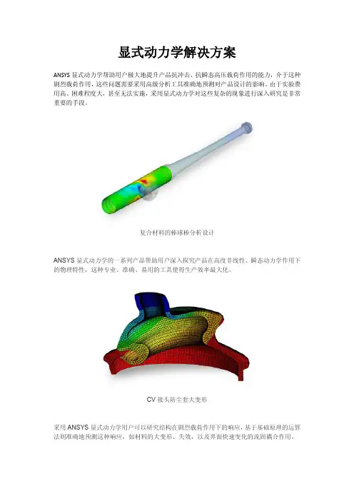
显式动力学解决方案ANSYS显式动力学帮助用户极大地提升产品抗冲击、抗瞬态高压载荷作用的能力，介于这种剧烈载荷作用，这些问题需要采用高级分析工具准确地预测对产品设计的影响。

由于实验费用高、困难程度大，甚至无法实施，采用显式动力学对这些复杂的现象进行深入研究是非常重要的手段。

复合材料的棒球棒分析设计ANSYS显式动力学的一系列产品帮助用户深入探究产品在高度非线性、瞬态动力学作用下的物理特性，这种专业、准确、易用的工具使得生产效率最大化。

CV接头防尘套大变形采用ANSYS显式动力学用户可以研究结构在剧烈载荷作用下的响应，基于基础原理的运算法则准确地预测这种响应，如材料的大变形、失效，以及界面快速变化的流固耦合作用。

承受剧烈载荷的物理问题作用时间非常短暂，一般是毫秒乃至微秒级，而这类问题需要显式动力学产品进行仿真计算。

对于涉及高度非线性、接触状态改变以及材料的破坏断裂，显式算法比隐式算法更加容易求解。

我们提供了完全自主的产品设置来满足这些问题的需求，解决显式动力学问题的三个各具优势的产品分别是：ANSYS Explicit STR，ANSYS Autodyn 和ANSYS LS-DYNA。

显式动力学解决方案功能特点承受剧烈载荷的物理问题作用时间非常短暂，一般是毫秒乃至微秒级，而这类问题需要显式动力学产品进行仿真计算。

对于涉及高度非线性、接触状态改变以及材料的破坏断裂，显式算法比隐式算法更加容易求解。

我们提供了完全自主的产品设置来满足这些问题的需求，解决显式动力学问题的三个各具优势的产品分别是：ANSYS Explicit STR，ANSYS Autodyn和ANSYS LS-DYNA。

广泛的应用功能ANSYS显式动力学帮助工程人员解决各种问题的仿真。

●短时间、复杂的接触、接触状态改变●准静态●高速和超高速撞击s●剧烈载荷作用下的大变形问题●材料失效●材料断裂●侵彻机理●空间碎片撞击（超高速）●体育器材设计●非线性塑形响应的加工制造●跌落试验及其他低速撞击●爆炸●爆炸成形●爆轰波结构耦合卷曲-复杂接触飞机撞击-材料失效建筑物内部爆炸载荷作用高级双向CAD接口本地CAD软件中的几何模型可以直接用于ANSYS显式动力学分析，不需要转换成中间格式（如IGES格式），不会丢失任何参数和设计信息。

Discrete Mathematics and Theoretical Computer Science1,1997,229–237On the bialgebra of functional graphs and differential algebrasMaurice GinocchioLaboratoire de Physique Th´e orique et Math´e matique,Universit´e Paris7,Tour Centrale-3`e me´e tage,2,place Jussieu, F-75251Paris Cedex05,FranceE-Mail:mag@ccr.jussieu.fr1IntroductionWe have already described the expansion of∆Σλi∂i,i.e.the powers of a Lie operator in any dimension, in order tofind the expression of theflow of formal nonlinear evolution equations[1–3].In the one-dimensional case,the explicit expansion can be foundfirst in Comtet[4],and other aspects connected to the ordinary differential equations can be found in Leroux and Viennot[5]and Bergeron and Reutenauer [6].On the other hand,Grossman and Larson[7]introduced several Hopf algebras[8–10]of forests of rooted labeled trees to express the product offinite dimensional vectorfields.In this paper we concentrate us on the bialgebra G of functional graphs,i.e.graphs representing mappings offinite sets in themselves [11–15].We give only the results without proofs.In a forthcoming paper[16],we develop Hopf algebra structures,computing the antipode and giving detailed aspects and proofs.In Sect.1we consider a bialgebra structure on G and three interesting subalgebras:T the set of labeled forests;S the set of permutation graphs;and L the set of well labeled forests,i.e.with strictly decreasing labels on the chains toward the roots.Recall that the graded bialgebra L is sufficient for the calculus of the powers of one derivation[1],and it is extendable in a Hopf algebra,the element of which is known in the computer literature as‘heap ordered trees’.This bialgebra is useful to compute products of derivations or to transform differential monomials in differential algebras[17],and it is interesting to note that the elements L n(n edges)can be coded by the words(monomials)of the expansion of Q nq0q0q1q0q1q n1,where Q0q0q1is a noncommutative alphabet.We describe in particular the bialgebra L,first in the polynomial form by the‘factorial’monoid L0L0n n0,where L0n is the set of words in the expansion of Q n,and second,we establish the bijective correspondence between 1365–8050c1997Chapman&Hall230M.Ginocchio L and L.We show that the calculus are easier with L,and that the product on L can be expressed in a very natural way.For example,q0n Q n,hence the(exponential)generating function of all the elements of L.We describe principally the formalism in the general case G,and the calculus uses thefields F201 as well as characteristic zerofields K.In Sect.2,we describe the link with the graded differential algebra K U r0K U r and the graded algebra of differential operators K U D r0K U r D r,where U u1u2uββ1uβαα0β1is a set of indeterminates,D∂0∂1and the differential indeterminates uβασ1σp∂σ1∂σpuβαgenerate K U r[17].This shows that the above Q-calculus,which is a kind of‘dissection’on functional graphs can be used as pre-calculus in differential algebras as well as in discrete dynamical systems[18].2Bialgebra Based on the Semi-group of Functional Graphs2.1T ypes of Functional GraphsIn this paper,a connected functional graph will be called excycle[13,15].In the area of discrete dynamical systems,an excycle is known as a basin of attraction.Consider several graded andfiltered sets of labeled functional graphs(i)E(resp.G)the set of excycles(resp.functional graphs)and designated by G n(resp.G n),the set offunctional graphs having(resp.having at most)n1nodes for n0(ii)R(resp.T)the set of labeled arborescences(resp.forests).(iii)C(resp.S)the set of cycles(resp.permutation graphs).(iv)A(resp.L)the set of well labeled arborescences(resp.forests),i.e.with strictly decreasing labels on the chains toward the root(s).As in(i),we consider for(ii)–(iv)graduations andfiltrations.2.2Free Representation by Q-polynomialsLet G n be the semigroup of mappings of12n in itself(‘Semigroup of endofunctions’), Card G n n n and the subsemigroups,T n f;f G n f n f n1(i.e.f acyclic and Card T n n1n1,S n the symmetric group and Card S n n!L n f;f G n f i i(i.e.f subdiagonal and Card L n n!.We have the well known bijections F F:G n G n T n T n S n S n L n L n.Let Q q0q1be a noncommutative alphabet,Q0q0Q with q0noncommuting with the q i’s,Q n q1q2q n Q0n q0Q n and Q(resp.Q0),the corresponding free monoids.Taking F201as thefield,consider(i)the G n module F2Q n by the F2linear incidence matrix action of f G n as l f q i q f i hence l f l gl f g.On the bialgebra of functional graphs231 (ii)the generating monomial associated with f.By morphism extension,denoted again by l f,we defineQ f q f1q f2q f n l f Qιn1where Qιn q1q2q n is associated with the identityιn of G n and Qι01One again has l f l g l f g.For the following we consider(iii)The graded subsets of Q as G G n n0T T n n0S S n n0L L n n0respectively associated with G,T,S and L,with G0T0S0L01(iv)The corresponding graded F2-modules:F2G F2T F2S F2L admit components of degree n which are,respectively,G n T n S n L n modules,withdimF2G n n n dimF2T n n1n1dimF2S n dimF2L n n!(v)We will denote by R n one of the above subsemi-groups of G n(or of another category). Similarly,let R R n n0resp F2R n0F2R n be the corresponding graded subsets of Q(resp. graded F2-modules ofF2G n0F2G n.2.3Virtual Root and External ProductLet f G n I0be the set offixed points of f and H0a subset of I0,and set p q r;p r q if p q and/0otherwise.Define f0:1n0n such that f0i f i if i H0and f0i0if i H0The‘0’is the label of a virtual root added to the graph representation of f,and we will say that H0is‘confined in0’,which is a fixed point of f0We call‘extended endofunctions’such functions f0,denote by G0n0n1n their set, and we consider G n as a subset of G0n Similarly,we will have T0n T n S0n S n L0n L n Consequently, adding q0,we get the extended graded sets G0G0n n0the extended graded F2-module F2G0 n0F2G0n and their substructures F2T0F2S0F2L0Now letφG0mχ0be the characteristic function of H0φ10,and writeQφlφQιm qφ1qφ2qφmm ∏i1qφi(cf.Figures1and2).WithψG0n,consider the F2-bilinear product in F2G0defined byQφQψQψm∏i1qφi nχ0i q0q1q n12On the right-hand side we have a sum of concatened monomials,and on the right factor the substitutions q0q0q1q n and q h q h n when h0232M.Ginocchio On the other hand,the product belongs to F2G0m n This external product is associated with unit1and F2G0is‘.’graded.To see this consider i j k being0three homogeneous polynomials,A A q0;q i F2G0mB B q0;q j F2G0nC C q0;q k F2G0pthen by(2)A B B q0;q j A q0q1q n;q i n3 and so,using deg B C n p,A q0;q iB q0;q jC B q0;q j A q0q1q n;q i n CCB q0q1q p;q j p A q0q1q p q1p q n p;q i n pA q0;q i CB q0q1q p;q j pA q0;q iB q0;q j CMoreover,because T n S n L n are subsemi-groups of G n one can see that F2R0F2T0F2S0F2L0are‘.’graded subalgebras of F2G0HenceProposition1Let the sequence G0m m1of the sets of the extended endofunctions in12m and Q0q0q1be a noncommutative alphabet.ForφG0m let Qφ∏m i1qφi be the generating monomial ofφand the graded module F2-module F2G0n0F2G0n on F201generated by all the φsThen F2G0is a graded algebra for the associative product with unit1QφQψQψm∏i1qφi nχ0i q0q1q n1whereψG0n andχ0is the characteristic function ofφ10Moreover,if R0m m1is a sequence of subsets associated with subsemi-groups of the sequence G0m m1, then F2R0n0F2R0n is a graded subalgebra of F2G02.4Splitting Operatorδn F2G0This operator substitutes the n-coproduct∆n of the Leibniz–Lie type.Associate to A Q0the left linear operatorτn A acting on B Q0,such that,if A G0m B G0n,then Bτn A BA if degB n,and0 otherwise,where BA is the concatenation of B and A.(i)Now let f G m and H0as in Sect.3,and notefirst that ifτn is viewed as acting on f,then for i1m one hasτn f i n f i n,and by f0i ¯χ0i f i one hasτn f0i n¯χ0i f0i n,where¯χ01χ0According to(2),define forφG0mδn Qφτnm∏i1qφi nχ0i q0q1q n14If d0Card H0the expansion(4)gives a sum of n1d0generating monomials of functionsψκof n1n m into0n1n m,and the corresponding functional graphs factorized in commutative excycles.On the bialgebra of functional graphs233 The operatorδn A is left linear on F2G0,and(2)can be writtenQφQψQψδn Qφ5 (ii)Moreover,δp is a graded antimorphism for‘’δp A Bδp Bδp n A6 where n degB and p N.For this to compute with(5)and A B C as in Sect.3,Cδp A B A B C A B C B Cδp n A Cδp Bδp n A.If p0we recover A B Bδn A and Bδk A0if k degB(iii)Also,δn is a powerδnδnδδ1δ017 For this to compute,δpδn A q0;q iδpτn A q0q1q n;q i nτn p A q0q1q p q1pq n p;q i n pδn p A q0;q i.(iv)Define the left linear operatorµin F2G0by the expansionµ∑n0δn8By left linear action ofµA on F2G0,we get A B BµA for A B F2G0with the antimorphism propertyµA BµBµA9 which express the associativity of‘’.Proposition2Let A F2G0m B F2G0n Then the splitting linear operatorδp defined left linearly by Bδp A A B if p=n,and0otherwise,verifiesδpδp withδδ1δ01andδp A Bδp Bδp n A Moreover,µ∑n0δn is an antimorphism in F2G0such that A B BµA2.5Exponential Generating Function of the Monomials of L0All the words of L0n(i.e.subdiagonals)are obtained from the expansion of Q n q0q0q1q0q1 q n1F2L0and Q01By equation(3),one has Q m Q n Q m n,and if A F2L0m B F2L0n we have A B F2L0m n,and then we recover that F2L0is stable for the product‘’.Because Q1q0,the associativity givesQ n q0n10 With the Q[[t]]-modules on L0,one has the exponential generating functionexp tq0∑n0t nn!Q n11exp sq0exp tq0exp s t q0234M.Ginocchio2.6ExamplesConsider equations (4)and (5)for Q ψq n 0.2.6.1Rooted T rees with n=1δq 20q 1τq 0q 12q 2τq 0q 0q 2τq 0q 1q 2τq 1q 0q 2τq 1q 1q 2(Figure 3)q 20q 1q 0q 0q 0q 12q 2q 30q 2q 20q 1q 2q 0q 1q 0q 2q 0q 1q 1q 2(Figure 4)2.6.2Excycles with n=2δ2q 23q 1q 0τ2q 25q 3q 0q 1q 2τ2q 25q 3q 0τ2q 25q 3q 1τ2q 25q 3q 2(Figure 5)q 23q 1q 0q 20q 20q 25q 3q 0q 1q 2q 20q 25q 3q 0q 20q 25q 3q 1q 20q 25q 3q 2(Figure 6)3Differential Algebra3.1Differential indeterminatesLet D ∂0∂1where ∂α∂∂ξαthe αth canonical derivation in S K ξthe algebra of formal power series in ξξ0ξ1,where K is a characteristic zero field.If S N N is the set U u 1u 2u ββ1u αβα0β1with u αβS consider U as a set of indeterminates,u αβσ1σp ∂σ1∂σp u αβasdifferential indeterminates,replace S N N by KU ,and consider the graded differential algebra K Ur 0K U r and the graded algebra of differential operators K U D r 0K U r D r.To each W F 2R 0we associate the differential operator W U U D ;for example,with W r U K U r one hasW UW 0UW 1Uα∂αW 2Uαβ∂α∂βW 0U∑r 1W r U D r12We will use now the summation convention.3.2Brackets in K UDefine for u v wU the multilinear operations valued in K U .3.2.1Arborescent Brackets (Valued in K U 1)u v uv w u vβu αv βα,henceu v Du αv βα∂β(1fixed point sent to ‘0’)uv wγu αv βw γαβ,henceu v Du αv βw γαβ∂γ13Also,for AK UrBK UsA Bβ1βsA α1αr B β1βsα1αr3.2.2Circular Brackets (Valued in K U 0)uu αα(1fixed point),u vu ααv ββ(2fixed points)u vu αβv βα2cycleu v wu αγv βαw γβ3cycle14On the bialgebra of functional graphs 2353.2.3Mixed Brackets (Valued in K U 0)Let E be a proper excycle (i.e.with no fixed point);we can write it EA i 1A i 2A i p ,where the A i k ’s are arborescences with root i k If in each arborescence A i k is reduced to its root i k ,we recover simply acycle Ei 1i 2i p Now let F k be the forest under i k ,i.e.obtained by cutting the root of A i k ,and defined with F i k U F i k u j ;j N i k ,where N i k is the set of nodes of F i k :E Uu F i 1i 1u F i 2i 2u F i pi pF i 1U u i 1α1αp F i 2U u i 2α2α1F i p U u i p αp αp13.3Action of F 2R 0Moreover,F 2R 0operates K -linearly in K U with values in K U D .For this let φG 0m H 0φ1for j 0m I 1m ,and H u β1u β2u βm U ,a word on U of length m .Then the action isQ φ∏i Iq φiQ φH∏j I∏i H j∂αiu αj βj∏k H 0∂αk15The differential monomial Q φH is such that u βj is associated with j in the domain I of φIf d j is the degree in q j (in-degree of the node labeled by ‘j ’),then u αj βj is derived d j times and the indices of derivation are related to the places of the q j ’s in the word.Similarly,the differential operator D r is characterized by the number r (degree of the root)of the q 0’s and their places.So we can summarize:In a word A R 0where q j is at the place (i),then in A H the j th letter of H is derived according to i,i.e.∂αi acts.One has,in particular,taking H u 1u 2:Arborescent brackets 1U 1q 0U u 1α1∂α1u 1Dq 0q 0U u 1α1u 2α2∂α1∂α2u 1u 2D 2q 0q 1U u 1α1α2u 2α2∂α1u 2u 1D q 3q 3q 0U u 1α1u 2α2u 3α3α1α2∂α3u 1u 2u 3Dq 0q 0q 2q 2U u 1α1u 2α2α3α4u α33u α44∂α1∂α2u 1u 3u 4u 2D 2Circular brackets q 1U u 1α1α1u 1q 1q 2U u 1α1α1u 2α2α2u 1u 2q 2q 1U u 1α1α2u 2α2α1u 1u 2q 3q 1q 2U u 1α1α3u 2α2α1u 3α3α2u 1u 2u 33.4Product of Differential OperatorsThe product (2)on words with correspondence (15)gives the product of differential operators.We state,without proof,Proposition 3Let the graded differential algebra K U r 0K U r and the graded algebra of differ-ential operators K U D r 0K U r D r Let φG 0m I 1m H j φ1j for j 0m and H u β1u β2u βm a word on U of length m.Then the mapping of F 2G 0into K U D which associates to the generating monomial Q φ∏i I q φi of φthe differential operator Q φH ∏j I ∏i H j ∂αi u αj βj ∏k H 0∂αk236M.Ginocchio is a morphism,such that ifψG0n and K is a word on U of length n,one has QφH QψK QφQψKH, where KH is the concatenation of K and H.ExampleA q0B q2q1q0H u4K u1u2u3A B q2q1q0q0q1q2q3q2q1q0q0q2q1q0q1q2q1q0q2q2q1q0q3(Figure7)A H u1DB K u1u2u3DA HB K u1u2u3u4D2u4u1u2u3D u1u2u4u3DObserve that:u4u1u2u3D u1α1α2α4u2α2α1u3α3u4α4∂α3u1α1α2u2α2α1α4u3α3u4α4∂α3which corresponds to q2q1q0q1q2,i.e.the second and third terms in the graph expansion. AppendixTo view Figures1–7,click here.To return to the main paper,click on the red box.References[1]Ginocchio,M.(1995).Universal expansion of the powers of a derivation,Letters in Math.Phys.34(4),343–364.[2]Ginocchio,M.and Irac-Astaud,M.(1985).A recursive linearization process for evolution equations.Reports on Math.Phys.21,245–265.[3]Steeb,W.H.and Euler,N.(1988).Nonlinear Evolution Equations and Painlev´e Test.World Scien-tific.[4]Comtet,L.(1973).Une formule explicite pour les puissances successives de l’op´e rateur de d´e rivationde m.Roy.Acad.Sci.276A,165–168.[5]Leroux,P.and Viennot,G.(1986).Combinatorial resolution of systems of differential equations I:ordinary differential equations.Actes du colloque de combinatoire´e num´e rative,Montr´e al.Lecture Notes in Mathematics1234,pp.210–245.Springer-V erlag.[6]Bergeron, F.and Reutenauer, C.(1987).Une interpr´e tation combinatoire des puissances d’unop´e rateur diff´e rentiel lin´e aire.Ann.Sci.Math.Quebec11,269–278.[7]Grossman,R.and Larson,R.G.(1989).Hopf-algebraic structures of families of trees.J.Algebra126,184–210.[8]Joni,A.A.and Rota,G.C.(1979).Coalgebras and bialgebras in combinatorics.Studies.in Appl.Math.61,93–139.On the bialgebra of functional graphs237 [9]Nichols,W.and Sweedler,M.E.(1980).Hopf algebras and combinatorics,in‘Umbral calculus andHopf algebras’.Contemp.Math.6.[10]Sweedler,M.E.(1969).Hopf Algebras.Benjamin.[11]Berge,C.(1983).Graphes.Gauthier-Villars.[12]Comtet,L.(1974).Advanced Combinatorics.Reidel.[13]Denes,J.(1968).On transformations,transformation-semigroups and graphs.In Erd¨o s-Katona,ed-itor,Theory of Graphs.Academic Press,pp.65–75.[14]Foata,D.and Fuchs,A.(1970).R´e arrangements de fonctions et d´e b.Theory8,361–375.[15]Harary,F.(1959).The number of functional digraphs.Math.Annalen138,203–210.[16]Ginocchio,M.On the Hopf algebra of functional graphs and differential algebras.Discr.Math.Toappear.[17]Kaplansky,I.(1976).Introduction to Differential Algebras.Springer-V erlag.[18]Robert,F.(1995).Les syst`e mes Dynamiques Discrets.Springer-V erlag.。

LANCZOS-BASED EXPONENTIAL FILTERINGFOR DISCRETE ILL-POSED PROBLEMSD.CAL VETTI∗AND L.REICHEL†In memory of R¨u diger Weiss.Abstract.We describe regularizing iterative methods for the solution of large ill-conditioned linear systems of equations that arise from the discretization of linear ill-posed problems.The regularization is specified by afilter function of Gaussian type.A parameterµdetermines the amount of regularization applied.The iterative methods are based on a truncated Lanczos decomposition and thefilter function is approximated by a linear combination of Lanczos polynomials.A suitable value of the regularization parameter is determined by an L-curve puted examples that illustrate the performance of the methods are presented.Key words.iterative method,regularization,exponentialfilter functionAMS subject classifications.65F22,65F10,65D151.Introduction.This paper is concerned with the computation of an approxi-mate solution of linear systems of equationsAx=˜g,A∈n×n,˜g∈n,(1)where A is a large symmetric matrix with many eigenvalues of different orders of magnitude close to the origin;some of the eigenvalues may vanish.The available right-hand side vector˜g is assumed to be an approximation of an unknown vector g′in the range of A.The difference(2)e:=˜g−g′may stem from measurement or discretization errors and will be referred to as noise. The vector˜g is not required to be in the range of A.Linear systems of equations with these properties arise when discretizing linear ill-posed problems,such as Fredholm integral equations of thefirst kind with a smooth symmetric kernel.Following Hansen[14],we refer to such linear systems of equations as linear discrete ill-posed problems.This paper presents new iterative methods for the solution of large linear discrete ill-posed problems with a symmetric matrix,which may be definite,indefinite or singular.Consider the consistent linear system of equations with the noise-free right-hand side g′,(3)Ax=g′,associated with(1).We would like to determine the solution of minimal Euclidean norm,denoted by x′,of this system.However,the right-hand side g′in(3)is not available.Therefore,we seek to determine an approximation of x′by computing anapproximate solution of the linear system of equations (1)with known right-hand side ˜g .Due to the noise e in ˜g and the severe ill-conditioning of the matrix A ,straight-forward solution of (1)typically does not yield a meaningful approximation of x ′.In order to facilitate the computation of a meaningful approximation of x ′,one generally replaces the discrete ill-posed problem (1)by a related problem that is less sensitive to the noise e in ˜g ,and then solves the problem obtained for an approximation of x ′.This replacement is referred to as regularization.We propose to replace the discrete ill-posed problem (1)by the least-squares problemmin x ∈nAx −ϕµ(A )˜g ,(4)where · denotes the Euclidean vector norm and ϕµ(t )is a filter function of Gaussian type,ϕµ(t ):=1−exp(−µt 2).(5)It is the purpose of this function to “filter out”the contributions of the noise e in ˜g to the computed solution.The nonnegative regularization parameter µdetermines how much noise is filtered out.Regularization by filtering out noise in the given data ˜g is sometimes referred to as prewhitening;see Louis [16]for a recent discussion of prewhitening and its relation to other regularization methods.Let A †denote the Moore-Penrose pseudo-inverse of the matrix A .The least-squares solution of minimal Euclidean norm of (4)is given byx µ=ϕµ(A )A †˜g .(6)Note that x ∞=A †˜g ,i.e.,when µ=∞the minimal-norm solution of (4)agrees with the minimal-norm least-squares solution of (1).This solution generally is a poor approximation of x ′,because the noise e in the right-hand side ˜g is not filtered out.On the other hand,the choice µ=0filters out too much;both e and ˜g are filtered out and we obtain x 0=0,which in general is a poor approximation of x ′.The determination of a suitable value of the regularization parameter is an important problem.Hansen[12]proposed that an L-curve be used for this purpose.Section 4describes how the L-curve criterion conveniently can be used for the iterative methods of the present paper.The influence of the filter function on the solution x µfor 0<µ<∞can easily be seen by substituting the spectral factorizationA =U n Λn U ∗n ,U ∗n U n =I n ,Λn =diag[λ1,λ2,...,λn ],(7)into (6).Here I n is the n ×n identity matrix and the superscript ∗denotes transpo-sition.For future reference,we introduce the index setsJ 0(A ):={j :λj =0},J 1(A ):={j :λj =0}.(8)Let U n have columns u j and defineδj :=u ∗j ˜g,1≤j ≤n.Then equation (6)can be expressed asx µ= j ∈J 1(A )ϕµ(λj )δjThis representation of xµshows that for0<µ<∞,eigenvector components of xµassociated with eigenvalues of small magnitude are damped,while eigenvector com-ponents associated with eigenvalues of large magnitude are not damped significantly. The smaller the value ofµ,the more damping.Application of thefilter function(5)to the solution of ill-posed problems was proposed in[3].Other choices offilter functions have been described in the literature. For instance,the simplest form of Tikhonov regularization applied to(1)yields the linear system of equations1(A2+(10)1+µt2andµ>0is the regularization parameter.Note that whenµt2is sufficiently small, the exponentialfilter functionϕµ(t)is an accurate approximation of the Tikhonov filter function(10).On the other hand,forµfixed,the Tikhonovfilter function has singularities at the points t:=±i/√−1,while the exponentialfilter function(5)is analytic in thefinite complex plane.We refer to[5]for further discussions on thefilter function(10).Numerical examples that compare thefiltering properties of the exponential and Tikhonovfilter functions,as well as of thefilter function defined by truncated singular value decomposition,are presented in[1].The present paper develops an iterative method for computing an approximation of xµby determining polynomial approximants of the function t−1ϕµ(t).The ap-proximants are expressed as a linear combination of orthogonal polynomials that are determined by the Lanczos process when applied to the matrix A with initial vector ˜g.The rapid convergence of the polynomial approximant follows from the fact that the function t−1ϕµ(t)is analytic in the whole complex plane.We remark that if a bounded interval[a,b]that contains the spectrum of the ma-trix A is known,then it is possible to determine polynomial approximants of t−1ϕµ(t) on[a,b]by expanding this function in terms of Chebyshev polynomials for this inter-val.An iterative method based on this approach is presented in[4].This paper is organized as follows.Section2describes a new iterative method for approximating the vector xµdefined by(6)for afixed value of the regularization parameterµ>0.A modification of this method that secures that the computed approximate solutions of(4)are orthogonal to the null space of A is presented in Section3.The choice of a suitable value of the regularization parameterµis discussed in Section4,and a few computed examples are presented in Section5.Finally,Section 6contains concluding remarks.2.An exponentiallyfiltering iterative method.We derive an iterative method based on the Lanczos process for computing approximations of the vector xµdefined by(6).The method determines a polynomial approximant of the analytic3functionψµ(t):= t−1(1−exp(−µt2)),t=0,0,t=0.(11)Note that the solution(6)of the least-squares problem(4)can be expressed asxµ=ψµ(A)˜g.(12)Application of m steps of the Lanczos process to the matrix A with initial vector ˜g yields the decompositionAQ m=Q m T m+q′m e∗m,(13)where the matrix Q m=[q0,q1,...,q m−1]∈n×m satisfies Q∗m Q m=I m and Q m e1=˜g/ ˜g ,the matrix T m∈m×m is symmetric and tridiagonal with nonvanishing sub-diagonal elements,the vector q′m∈n is orthogonal to the columns of Q m,and e j denotes the j th axis vector.Throughout this paper,we assume that the Lanczos pro-cess does not break down during thefirst m steps.In the rare event of a breakdown, the formulas derived can be simplified in an obvious manner.It follows from(13)that the columns q j of the matrix Q m span the Krylov sub-spaceK m(A,˜g):=span{˜g,A˜g,A2˜g,...,A m−1˜g}(14)and that they satisfy a three-term recurrence relation.In particular,the q j can be expressed asq j=πj(A)˜g/ ˜g ,j=0,1,2,...,(15)whereπj is a polynomial of degree j.We refer to the q j as Lanczos vectors and to the πj as Lanczos polynomials.Since the Lanczos vectors satisfy a tree-term recurrence relation,so do the Lanczos polynomials;see,e.g.,Golub and Van Loan[8]for details on the Lanczos process.We seek to determine an approximation of xµof the formxµ,m=m−1j=0γj,m q j,γj,m∈.(16)In view of(12),the problem of approximating xµby xµ,m is equivalent to the approx-imation ofψµby a linear combination of the Lanczos polynomials(15).We will use this equivalence to derive a numerical method for determining the coefficientsγj,m.Our numerical method is based on the fact that the Lanczos polynomials are orthogonal with respect to an inner product defined by a measure on the real axis.A discussion on Lanczos polynomials and Gauss quadrature rules can be found in[7]. We review relevant properties and assume for simplicity that the Lanczos process does not break down until n steps have been carried out.Then Lanczos decompositions of the form(13)exist for1≤m<n.Moreover,when m=n,the vector q′m in(13) vanishes and we obtainA=Q n T n Q∗n.(17)4Substituting(17)into(12)givesxµ=ψµ(Q n T n Q∗n)˜g= ˜g Q nψµ(T n)e1=n−1 j=0γj q j,whereγj:= ˜g e∗j+1ψµ(T n)e1,0≤j<n.(18)Introduce the inner product<f1,f2>:=1˜g 2(πj(A)˜g)∗(πk(A)˜g)=q∗j q k= 1,j=k, 0,j=k.(21)Consider the spectral decompositionT n=W nΛn W∗n,W∗n W n=I n,(22)where the diagonal matrixΛn is the same as in(7).Analogously to(20),we definef j(T n):=W n diag[f j(λ1),f j(λ2),...,f j(λn)]W∗n,j=1,2,(23)and it follows from(17)thatf j(A)=Q n f j(T n)Q∗n,j=1,2.(24)Substituting(24)and(23)into(19)yields<f1,f2>=e∗1f1(T n)f2(T n)e1=e∗1W n diag[f1(λ1)f2(λ1),f1(λ2)f2(λ2),...,f1(λn)f2(λn)]W∗n e1=nj=1f1(λj)f2(λj)ω2j,ωj:=e∗1W n e j.(25)Following Golub and Meurant[7],we write the sum(25)as a Stieltjes integral.For this purpose,define the nonnegative measuredω(t):=nj=1δ(t−λj)ω2j,(26)whereδdenotes the Diracδ-function.Then<f1,f2>=nj=1f1(λj)f2(λj)ω2j= ∞−∞f1(t)f2(t)dω(t).(27)5We are now in a position to express the coefficients(18)in terms of Stieltjes integrals.It follows from(15)and(17)that1e∗j+1ψµ(T n)e1=q∗jψµ(A)q0=xµ,m lives increases with m,and because the accuracy of the Gauss quadrature rules (33)increases with m for eachfixed j.Bounds for xµ,m−xµ can be derived as follows.Express the functionψµ(t)in[a,b]as a series of Chebyshev polynomials of thefirst kind for this interval.Bounds for the oefficients in this expansion can be derived by techniques discussed in[5].Sinceψµ(t)is analytic in thefinite complex plane,the terms in the series converge to zero faster than geometrically.Druskin and Knizhnerman[6]show how the bounds for these terms can be used to bound the error xµ,m−xµ .This approach shows that the error decreases faster than geometrically as m increases.3.A modified iterative method.The representation(9)shows that xµis orthogonal to the null space of A.We describe a modification of the method of Section 2with the property that the computed approximate solutions of(4),denoted byˆxµ,m, also are orthogonal to the null space of A.Since the matrix A is symmetric,its null space and range are orthogonal.We therefore require the approximate solutionsˆxµ,m to be in the range of A.Let R(A)denote the range of A and defineˆg:=A˜g.(36)Apply m steps of the Lanczos process to the matrix A with initial vectorˆg.Assuming that the Lanczos process does not break down,we obtain,analogously to(13),the decompositionAˆQ m=ˆQ mˆT m+ˆq′m e∗m,(37)where the matrixˆQ m=[ˆq0,ˆq1,...,ˆq m−1]∈n×m satisfiesˆQ∗mˆQ m=I m andˆQ m e1=ˆg/ ˆg ,the matrixˆT m∈m×m is symmetric and tridiagonal with nonvanishing sub-diagonal elements,and the vectorˆq′m∈n is orthogonal to the columns ofˆQ m.It follows from(37)and(36)that the columnsˆq j of the matrixˆQ m span the Krylov subspace K m(A,A˜g),which is in R(A).We determine an approximation of xµof the formˆxµ,m=m−1j=0ˆγj,mˆq j,ˆγj,m∈,(38)where we note thatˆxµ,m∈R(A)for any choice of coefficientsˆγj,m.Introduce the functionˆψµ(t):= t−2(1−exp(−µt2)),t=0, 0,t=0.This function is discontinuous at t=0whenµ=0.The solution(6)of the least-squares problem(4)can be expressed asxµ=ˆψµ(A)ˆg,where we defineˆψµ(A):=U n diag[ˆψµ(λ1),ˆψµ(λ2),...,ˆψµ(λn)]U∗n.Analogously to the representation(34)of the coefficientsγj,m,we letˆγj,m:= ˆg e∗j+1ˆψµ(ˆT m)e1,0≤j<m,(39)whereˆψµ(ˆT m)is defined similarly asˆψµ(A).Substituting(39)into(38)yieldsˆxµ,m= ˆg ˆQ mˆψµ(ˆT m)e1,(40)analogously to(35).74.Determination of the regularization parameter.In many discrete ill-posed problems that arise in applications a suitable value of the regularization pa-rameter µis not known a priori.A method for determining such a value based on the discrepancy principle is described in [4].This method requires that the norm of the noise e be known.The L-curve criterion for determining a suitable value of the regularization parameter,proposed by Hansen [12],does not require knowledge of e .This method is based on comparing the norm of the computed approximate solution with the norm of the associated residual vector.We focus primarily on the method of Section 2,which determines approximate solutions x µ,m given by (35).The associated residual vector is defined byr µ,m :=˜g −Ax µ,m .(41)Before studying the behavior of x µ,m and r µ,m as a function of µ,we inves-tigate how the norm of the solution x µof (4)and of the associated residual vectorr µ=˜g −Ax µ(42)changes with µ.Throughout this section N (A )denotes the null space of A .Theorem 4.1.Let x µbe defined by (6),let ˜g N (A )denote the orthogonal pro-jection of ˜g onto N (A ),and assume that ˜g =˜g N (A ).Then the residual vector (42)associated with x µsatisfiesr 0 = ˜g ,(43)lim µ→∞r µ = ˜g N (A ) .(44)Moreover, r µ is a strictly decreasing function of µfor µ≥0.Proof .Substituting the representation (9)into (42)yieldsr µ 2=j ∈J 0(A )δ2j + j ∈J 1(A )(δj −φµ(λj )δj )2(45)=j ∈J 0(A )δ2j + j ∈J 1(A )exp(−2µλ2j )δ2j ,where the index sets J 0(A )and J 1(A )are defined by (8).Equations (43)and (44)follow from (45)and the observation thatj ∈J 0(A )δ2j = ˜g N (A ) 2.Differentiating (45)with respect to µyieldsr µ ddµ r µ <0for µ≥0.Hence, r µ is a strictly decreasing function of µ.Theorem 4.2.Let x µbe defined by (6)for µ≥0,and assume that ˜g =˜g N (A ).Thenx 0 =0,(47)lim µ→∞x µ = A †˜g .(48)8Moreover, xµ is a strictly increasing function ofµforµ>0.Proof.The representation(9)yieldsxµ 2= j∈J1(A)(1−exp(−µλ2j))2 δjdµ xµ >0forµ>0.We now show results analogous to Theorems4.1and4.2for the approximate solution(35)and the associated residual vector(41).Theorem4.3.The norm of the residual vector(41)can be expressed as rµ,m =( exp(−µT2m)e1 2+|e∗mψµ(T m)e1|2 q′m 2)1/2 ˜g , (50)where the matrix T m and vector q′m are defined by the Lanczos decomposition(13). In particular,r0,m = ˜g .(51)If the vector q′m in the Lanczos decomposition(13)vanishes,then rµ,m is a decreas-ing function ofµforµ≥0,andlimµ→∞ rµ,m =(j∈J0(T m)ω2j,m)1/2 ˜g ,(52)where the index set J0(T m)is defined by(31)and the Gaussian weightsω2j,m are determined by(30).In particular,when T m is nonsingular,J0(T m)=∅andlimµ→∞ rµ,m =0.Conversely,if q′m=0,thenlimµ→∞ rµ,m =(j∈J0(T m)ω2j,m+|e∗m T†m e1|2 q′m 2)1/2 ˜g .(53)Since e∗m T†m e1=0,the norm of rµ,m might not be a decreasing function ofµ.Proof.Substituting(35)and(13)into(41)yieldsrµ,m=˜g−AQ mψµ(T m)e1 ˜g =(Q m(I m−T mψµ(T m))e1−q′m e∗mψµ(T m)e1) ˜g . The orthogonality of the vector q′m to the columns of Q m yields(50).Substituting the spectral decomposition(29)of T m into(50)givesrµ,m 2=( j∈J1(T m)exp(−2µλ2j,m)ω2j,m+ j∈J0(T m)ω2j,m) ˜g 2(54)+( j∈J1(T m)˘ωj,mωj,mψµ(λj,m))2 q′m 2 ˜g 2,where theωj,m and˘ωj,m are given by(30).Setting q′m=0in this expression shows (51)and(52).Moreover,it follows from(54)that rµ,m is a decreasing function of µwhen q′m=0.Since the sub-and super-diagonal entries of T m are nonvanishing,it is easy to see that thefirst and last eigenvector componentsωj,m and˘ωj,m,given by(30),are9nonvanishing for all j.Therefore,the last term in(54)does not vanish when q′m=0. The observation thatlimµ→∞ j∈J1(T m)˘ωj,mωj,mψµ(λj,m)=limµ→∞j∈J1(T m)˘ωj,mωj,mλ−1j,m=e∗m T†m e1completes the proof.We have observed in computations that typically rµ,m decreases monotonically for0≤µ≤µ∗for someµ∗>0.For large values ofµ,the norm of rµ,m may increase withµ.This is illustrated by computed examples in Section5.Theorem4.4.Let xµ,m be given by(35)forµ≥0.Thenx0,m =0, (55)limµ→∞ xµ,m = ˜g (e ∗1(T†m)2e1)1/2.(56)Moreover, xµ,m is a strictly increasing function ofµforµ>0.Proof.The representation(35)of xµ,m yieldsxµ,m 2= ψµ(T m)e1 2 ˜g 2= j∈J1(T m)λ−2j,m(1−exp(−µλ2j,m))2ω2j,m ˜g 2.(57)Equation(55)follows by settingµ=0in(57).Lettingµ→∞in(57)yieldslimµ→∞ xµ,m2= j∈J1(T m)λ−2j,mω2j,m ˜g 2,which shows(56).Differentiation of(57)with respect toµshows that dwith Theorems4.3and4.4.For small values ofµthe slope of the graph is negative andof large magnitude.This indicates that an increase ofµgives a significant reduction in the norm rµ,m ,but xµ,m only increases slightly.For larger values ofµ,the graph typically has a negative slope of small magnitude.This indicates that an increase ofµonly gives a slight decrease of rµ,m ,but xµ,m may grow considerably.For even larger values ofµboth rµ,m and xµ,m might increase withµ.When the vector q′m=0, rµ,m is a decreasing function ofµ,cf.Theorem4.3, and the graph of the set L often looks like the letter“L”.Theorem4.3indicates that when q′m=0,the graph may be shaped like the letter“U”.We refer to the graph of the set L as the L-curve,whether q′m vanishes or not.Following the approach by Hansen[12],we choose a value of the regularization parameter in the vicinity of the point of largest curvature of the graph.The value ofµso determined seeks to achieve a small norm of the residual vector rµ,m and a fairly small norm of the computed approximate solution xµ,m.If the graph is“U-shaped”in the vicinity of the point of largest curvature,then it may be possible to reduce the error xµ.m−x′by increasing the value of m.We remark that the L-curve criterion may fail to determine a suitable value ofthe regularization parameter for certain problems.However,its simplicity and the fact that it for many problems gives a fairly good value of the the regularization parameter contribute to its popularity.For insightful discussions on the advantages and limitations of the L-curve criterion,we refer to[14,15].puted examples.This section describes numerical examples that illus-trate the performance of the exponentialfiltering method of Section2.The method of Section3performed in a similar manner.We therefore do not report experiments with the latter method.The only advantage of the method of Section3is that the approximate solutions determined are guaranteed to be orthogonal to the null space of A.Our implementation of the exponentialfiltering method of Section2stores the matrix Q m and vector q′m in the Lanczos decomposition(13),and reorthogonalizes the columns of Q m and q′m to secure numerical orthogonality.We compare this im-plementation with the MR-II method proposed by Hanke and use the implementation described in[9].The MR-II method is a minimal residual method that determines a sequence of approximate solutions˘x m∈K m(A,A˜g)of(1)that satisfyA˘x m−˜g =minx∈K m(A,A˜g) Ax−˜g ,m=1,2,....The iteration number m can be thought of as the regularization parameter.It is important to determine when to terminate the iterations with the MR-II method.Too few iterations gives a residual vector˘r m:=˜g−A˘x m of unnecessarily large norm,and too many iterations yields an approximate solution˘x m that is severely contaminated by propagated errors due to the error e in the right-hand side˜g.An analysis of the performance of the MR-II method is provided by Hanke[9].The MR-II method only requires storage of a few n-vectors at a time.The point setL d:={( ˘x m , ˘r m ):m=1,2,...}(59)determined by the iterates˘x m and associated residual vectors˘r m generated by the MR-II method is analogous to the set(58)for the exponentialfiltering method of Section2.Below we show log-log plots of the curves obtained by linear interpolation11between successive points in the set(59)and refer to these graphs as L-curves for the MR-II method.For many linear discrete ill-posed problems(1)these graphs are shaped like the letter“L”.Iterates˘x m associated with points close to the“vertex”of the graph are often suitable choices of approximate solutions of(1).This approach of choosing the regularization parameter for iterative methods is discussed in[10,11,14].We found that for many linear discrete ill-posed problems(1)the best possible approximations of the minimal-norm least-squares solution of the associated noise-free linear system of equations(3),denoted by x′,determined by the method of Section 2and by the MR-II method are of roughly the same quality.Moreover,the value of the regularization parameterµdetermined by the L-curve(58)and the number of iterations m determined by the L-curve for the MR-II method(59)often are adequate. Example5.1below provides an illustration.However,for some linear discrete ill-posed problems,the exponentialfiltering method of Section2implemented as described in the present section gives considerably better approximations of x′than the MR-II method.This is illustrated by Example5.2.All computed examples of this section are implemented in Matlab on a PC with a Pentium III processor.The unit roundoffisǫ≈2·10−16.Fig.1.Example5.1:Error xµj,60−x′ as a function of j for approximate solutions xµj,60determined by the exponentialfiltering method,whereµj:=100·(1.25)j−1,1≤j≤100.Example5.1.We are concerned with the solution of a linear system of equations of the form(1)with the matrix defined byA:=U300Λ300U∗300∈300×300,whereΛ300:=diag[1,2−3,3−3,...,300−3],(60)and U300is the orthogonal eigenvector matrix of a symmetric300×300matrix de-termined by discretizing a Fredholm integral equation of thefirst kind discussed by12050100150200250300−20020406080100120Fig.2.Example 5.1:Computed approximate solution x µ89,60by the exponential filtering method (continuous curve)and exact solution x ′of the noise-free linear system (3)(dash-dotted curve).Phillips [17].The discretization was carried out using Matlab code provided by Hansen[13].The eigenvectors u j have the property that the number of sign changes in the sequence {e ∗j u k }300j =1increases with the index k .This property is typical of matrices obtained by discretizing Fredholm integral equations of the first kind.Let x ′∈300represent the spike shown by the dash-dotted graph in Figure 2;only 10of the entries of the vector are nonvanishing.Define the noise-free right-hand side g ′:=Ax ′.Then x ′ =2.5·102and g ′ =4.3·101.Let the entries of the noise-vector e be normally distributed with zero mean and variance chosen so that e =1·10−3and define the contaminated right-hand side by ˜g :=g ′+e ,cf.(2).First consider the exponential filtering method of Section 2.We carry out 60steps of the Lanczos process and evaluate the norms of the approximate solutions x µj ,60and of the associated residual vectors r µj ,60for µj :=100·1.25j −1,1≤j ≤100.After the Lanczos decomposition (13)with m =60has been computed,we determine the spectral decomposition (29)of the symmetric tridiagonal matrix T 60generated by the Lanczos process.The norms r µj ,60 and x µj ,60 can then be computed quite inexpensively for each value of µj by using the formulas (54)and (57).Figure 1displays the error x µj ,60−x ′ for µj :=100·1.25j −1and 1≤j ≤100.The smallest error is achieved for j =89;we have µ89=3.4·1010.The continuous graph of Figure 2displays x µ89,60,the dash-dotted curve shows x ′.The latter figure shows x µ89,60to be a fairly good approximation of x ′.We have x µ89,60−x ′ =9.3·101.Figure 3shows the L-curve (58)for m =60and µj :=100·1.25j −1,1≤j ≤100.We have marked the point ( x µ89,60 , r µ89,60 )on the L-curve by “∗”.This point is located near the point of largest curvature of the L-curve.Thus,the value of the regularization parameter µassociated with the point of largest curvature on the L-curve is appropriate for linear system of equations of the present example.We turn to the MR-II method and compute approximate solutions ˘x m for 1≤1310110210310−410−310−210−110101Fig.3.Example 5.1:L-curve (58)for the exponential filtering method for m =60and µ=µj =10·1.25j −1,1≤j ≤100.The point ( x µ89,60 , r µ89,60 )on the curve is marked by “∗”.Fig.4.Example 5.1:Error ˘x m −x ′ as a function of m ,1≤m ≤100,for solutions ˘x m determined by the MR-II method.m ≤100.Figure 4shows the error ˘x m −x ′ for 1≤m ≤100.The smallest error is achieved for m =66.Figure 5shows the computed solution ˘x 66(continuous curve)and the exact solution x ′of the noise-free linear system of equations (3)(dash-dotted curve).The figure shows ˘x 66to be a fairly good approximation of x ′;we have ˘x 66−x ′ =9.9·101.This error is slightly larger than the error for the approximate14050100150200250300−20020406080100120Fig.5.Example 5.1:Computed approximate solution ˘x 66by the MR-II method (continuous curve)and exact solution x ′of the noise-free linear system (3)(dash-dotted curve).Fig.6.Example 5.1:L-curve for the MR-II method defined by the set (59)for 1≤m ≤100.Adjascent points are connected by straight lines.The point ( ˘x 66 , ˘r 66 )is marked by “∗”.solution x µ89,60determined by the exponential filtering method.Figure 6displays the L-curve associated with the MR-II method.The point ( ˘x 66 , ˘r 66 )is marked by “∗”.It is located at a point where the slope of the L-curve for the MR-II method changes the most,i.e.,at the “vertex”of the L-curve.15。

关于L_p-极曲率映像的几个不等式（英文）李新红;马统一【期刊名称】《数学季刊：英文版》【年(卷),期】2016(31)4【摘要】Zhu,Lü and Leng extended the concept of L_p-polar curvature image. We continuously study the L_p-polar curvature image and mainly expound the relations between the volumes of star bodies and their L_p-polar curvature images in this article. We first establish the L_p-affine isoperimetric inequality associated with L_p-polar curvature image. Secondly,we give a monotonic property for L_p-polar curvature image. Finally, we obtain an interesting equation related to L_p-projection body of L_p-polar curvature image and L_p-centroid body.【总页数】10页(P349-358)【关键词】star bodies;convex bodies;Lp-curvature image;Lp-polar curvature image【作者】李新红;马统一【作者单位】College of Mathematics and Statistics,Northwest Normal University;College of Mathematics and Statistics,Hexi University【正文语种】中文【中图分类】O184【相关文献】1.关于Lp-混合极投影体的几个不等式 [J], 胡妍;卢峰红2.Lp-新几何体极的几个不等式 [J], 朱保成;李妮3.关于L_p-极投影体Shephard问题的一个类似（英文） [J], 马统一4.关于L_p-混合仿射表面积的不等式(英文) [J], 朱先阳5.L_p-极投影Brunn-Minkowski不等式 [J], 赵长健;张荣森因版权原因，仅展示原文概要，查看原文内容请购买。