信号与系统实验报告4
- 格式:doc
- 大小:441.00 KB
- 文档页数:9
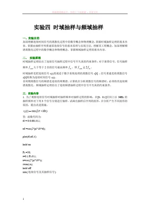
实验四 时域抽样与频域抽样一、实验目的加深理解连续时间信号的离散化过程中的数学概念和物理概念,掌握时域抽样定理的基本内容。
掌握由抽样序列重建原连续信号的基本原理与实现方法,理解其工程概念。
加深理解频谱离散化过程中的数学概念和物理概念,掌握频域抽样定理的基本内容。
二、 实验原理时域抽样定理给出了连续信号抽样过程中信号不失真的约束条件:对于基带信号,信号抽样频率sam f 大于等于2倍的信号最高频率m f ,即m sam f f 2≥。
时域抽样是把连续信号x (t )变成适于数字系统处理的离散信号x [k ] ;信号重建是将离散信号x [k ]转换为连续时间信号x (t )。
非周期离散信号的频谱是连续的周期谱。
计算机在分析离散信号的频谱时,必须将其连续频谱离散化。
频域抽样定理给出了连续频谱抽样过程中信号不失真的约束条件。
三.实验内容1. 为了观察连续信号时域抽样时抽样频率对抽样过程的影响,在[0,0.1]区间上以50Hz 的抽样频率对下列3个信号分别进行抽样,试画出抽样后序列的波形,并分析产生不同波形的原因,提出改进措施。
)102cos()(1t t x ⨯=π答: 函数代码为: t0 = 0:0.001:0.1;x0 =cos(2*pi*10*t0);plot(t0,x0,'r')hold onFs =50;t=0:1/Fs:0.1;x=cos(2*pi*10*t); stem(t,x); hold offtitle('连续信号及其抽样信号')函数图像为:)502cos()(2t t x ⨯=π同理,函数图像为:)0102cos()(3t t x ⨯=π同理,函数图像为:由以上的三图可知,第一个图的离散序列,基本可以显示出原来信号,可以通过低通滤波恢复,因为信号的频率为20HZ,而采样频率为50>2*20,故可以恢复,但是第二个和第三个信号的评论分别为50和100HZ,因此理论上是不能够恢复的,需要增大采样频率,解决的方案为,第二个信号的采样频率改为400HZ,而第三个的采样频率改为1000HZ,这样可以很好的采样,如下图所示:2. 产生幅度调制信号)200cos()2cos()(t t t x ππ=,推导其频率特性,确定抽样频率,并绘制波形。
《信号与系统》课程实验报告《信号与系统》课程实验报告一图1-1 向量表示法仿真图形2.符号运算表示法若一个连续时间信号可用一个符号表达式来表示,则可用ezplot命令来画出该信号的时域波形。
上例可用下面的命令来实现(在命令窗口中输入,每行结束按回车键)。
t=-10:0.5:10;f=sym('sin((pi/4)*t)');ezplot(f,[-16,16]);仿真图形如下:图1-2 符号运算表示法仿真图形三、实验内容利用MATLAB实现信号的时域表示。
三、实验步骤该仿真提供了7种典型连续时间信号。
用鼠标点击图0-3目录界面中的“仿真一”按钮,进入图1-3。
图1-3 “信号的时域表示”仿真界面图1-3所示的是“信号的时域表示”仿真界面。
界面的主体分为两部分:1) 两个轴组成的坐标平面(横轴是时间,纵轴是信号值);2) 界面右侧的控制框。
控制框里主要有波形选择按钮和“返回目录”按钮,点击各波形选择按钮可选择波形,点击“返回目录”按钮可直接回到目录界面。
图1-4 峰值为8V,频率为0.5Hz,相位为180°的正弦信号图1-4所示的是正弦波的参数设置及显示界面。
在这个界面内提供了三个滑动条,改变滑块的位置,滑块上方实时显示滑块位置代表的数值,对应正弦波的三个参数:幅度、频率、相位;坐标平面内实时地显示随参数变化后的波形。
在七种信号中,除抽样函数信号外,对其它六种波形均提供了参数设置。
矩形波信号、指数函数信号、斜坡信号、阶跃信号、锯齿波信号和抽样函数信号的波形分别如图1-5~图1-10所示。
图1-5 峰值为8V,频率为1Hz,占空比为50%的矩形波信号图1-6 衰减指数为2的指数函数信号图1-7 斜率=1的斜坡信号图1-8 幅度为5V,滞后时间为5秒的阶跃信号图1-9 峰值为8V,频率为0.5Hz的锯齿波信号图1-10 抽样函数信号仿真途中,通过对滑动块的控制修改信号的幅度、频率、相位,观察波形的变化。
信号与系统实验实验报告一、实验目的本次信号与系统实验的主要目的是通过实际操作和观察,深入理解信号与系统的基本概念、原理和分析方法。
具体而言,包括以下几个方面:1、掌握常见信号的产生和表示方法,如正弦信号、方波信号、脉冲信号等。
2、熟悉线性时不变系统的特性,如叠加性、时不变性等,并通过实验进行验证。
3、学会使用基本的信号处理工具和仪器,如示波器、信号发生器等,进行信号的观测和分析。
4、理解卷积运算在信号处理中的作用,并通过实验计算和观察卷积结果。
二、实验设备1、信号发生器:用于产生各种类型的信号,如正弦波、方波、脉冲等。
2、示波器:用于观测输入和输出信号的波形、幅度、频率等参数。
3、计算机及相关软件:用于进行数据处理和分析。
三、实验原理1、信号的分类信号可以分为连续时间信号和离散时间信号。
连续时间信号在时间上是连续的,其数学表示通常为函数形式;离散时间信号在时间上是离散的,通常用序列来表示。
常见的信号类型包括正弦信号、方波信号、脉冲信号等。
2、线性时不变系统线性时不变系统具有叠加性和时不变性。
叠加性意味着多个输入信号的线性组合产生的输出等于各个输入单独作用产生的输出的线性组合;时不变性表示系统的特性不随时间变化,即输入信号的时移对应输出信号的相同时移。
3、卷积运算卷积是信号处理中一种重要的运算,用于描述线性时不变系统对输入信号的作用。
对于两个信号 f(t) 和 g(t),它们的卷积定义为:\(f g)(t) =\int_{\infty}^{\infty} f(\tau) g(t \tau) d\tau \在离散时间情况下,卷积运算为:\(f g)n =\sum_{m =\infty}^{\infty} fm gn m \四、实验内容及步骤实验一:常见信号的产生与观测1、连接信号发生器和示波器。
2、设置信号发生器分别产生正弦波、方波和脉冲信号,调整频率、幅度和占空比等参数。
3、在示波器上观察并记录不同信号的波形、频率和幅度。
信号与系统实验报告一、实验目的(1) 理解周期信号的傅里叶分解,掌握傅里叶系数的计算方法;(2)深刻理解和掌握非周期信号的傅里叶变换及其计算方法;(3) 熟悉傅里叶变换的性质,并能应用其性质实现信号的幅度调制;(4) 理解连续时间系统的频域分析原理和方法,掌握连续系统的频率响应求解方法,并画出相应的幅频、相频响应曲线。
二、实验原理、原理图及电路图(1) 周期信号的傅里叶分解设有连续时间周期信号()f t ,它的周期为T ,角频率22fT,且满足狄里赫利条件,则该周期信号可以展开成傅里叶级数,即可表示为一系列不同频率的正弦或复指数信号之和。
傅里叶级数有三角形式和指数形式两种。
1)三角形式的傅里叶级数:01212011()cos()cos(2)sin()sin(2)2cos()sin()2n n n n a f t a t a t b t b t a a n t b n t 式中系数n a ,n b 称为傅里叶系数,可由下式求得:222222()cos(),()sin()T T T T nna f t n t dtb f t n t dtTT2)指数形式的傅里叶级数:()jn tn nf t F e式中系数n F 称为傅里叶复系数,可由下式求得:221()T jn tT nF f t edtT周期信号的傅里叶分解用Matlab进行计算时,本质上是对信号进行数值积分运算。
Matlab中进行数值积分运算的函数有quad函数和int函数。
其中int函数主要用于符号运算,而quad函数(包括quad8,quadl)可以直接对信号进行积分运算。
因此利用Matlab进行周期信号的傅里叶分解可以直接对信号进行运算,也可以采用符号运算方法。
quadl函数(quad系)的调用形式为:y=quadl(‘func’,a,b)或y=quadl(@myfun,a,b)。
其中func是一个字符串,表示被积函数的.m文件名(函数名);a、b分别表示定积分的下限和上限。
信号与系统实验报告
实验名称:信号与系统实验
一、实验目的:
1.了解信号与系统的基本概念
2.掌握信号的时域和频域表示方法
3.熟悉常见信号的特性及其对系统的影响
二、实验内容:
1.利用函数发生器产生不同频率的正弦信号,并通过示波器观察其时域和频域表示。
2.通过软件工具绘制不同信号的时域和频域图像。
3.利用滤波器对正弦信号进行滤波操作,并通过示波器观察滤波前后信号的变化。
三、实验结果分析:
1.通过实验仪器观察正弦信号的时域表示,可以看出信号的振幅、频率和相位信息。
2.通过实验仪器观察正弦信号的频域表示,可以看出信号的频率成分和幅度。
3.利用软件工具绘制信号的时域和频域图像,可以更直观地分析信号的特性。
4.经过滤波器处理的信号,可以通过示波器观察到滤波前后的信号波形和频谱的差异。
四、实验总结:
通过本次实验,我对信号与系统的概念有了更深入的理解,掌
握了信号的时域和频域表示方法。
通过观察实验仪器和绘制图像,我能够分析信号的特性及其对系统的影响。
此外,通过滤波器的处理,我也了解了滤波对信号的影响。
通过实验,我对信号与系统的理论知识有了更加直观的了解和应用。
V i (t)V 0(t)滤波电路实验 4 低通与高通滤波器一、实验目的1. 熟悉低通与高通滤波器的构成及其特性;2. 学会测量滤波器幅频特性的方法。
二、实验原理说明滤波器是一种能使有用频率信号通过而同时抑制(或大为衰减)无用频率信号的电子装置。
工程上常用它作信号处理、数据传送和抑制干扰等。
这里主要是讨论模拟滤波器。
以往这种滤波电路主要采用无源元件 R 、L 和 C 组成,60 年代以来,集成运放获得了迅速发展, 由它和 R 、C 组成的有源滤波电路, 具有不用电感、体积小、重量轻等优点。
此外,由于集成运放的开环电压增益和输入阻抗均很高,输出阻抗又低,构成有源滤波电路后还具有一定的电压放大和缓冲作用。
但是,集成运放的带宽有限,所以目前有源滤波电路工作频率难以做得很高,这是它的不足之处。
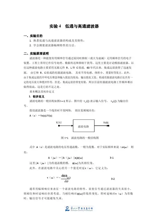
基本概念及初步定义 1. 初步定义滤波电路的一般结构如图4—1 所示。
图中的 v 1 (t ) 表示输入信号, v 0 (t ) 为输出信 号。
假设滤波器是一个线形时不变网络, 则在复频域内有: A (s )=Vo(s)/Vi(s)图 4-1 滤波电路的一般结构图式中 A (s )是滤波电路的电压传递函数,一般为复数。
对于实际频率来说(s=jω) 则有:A ( j ω)=│A ( j ω)│ejφ(ω)3-1这里│A ( j ω)│为传递函数的模, φ(ω)为其相位角。
此外,在滤波电路中关心的另一个量是时延τ(ω),它定义为:τ(ω)=- d ϕ(ω)(s ) d ω3-2通常用幅频响应来表征一个滤波电路的特性,欲使信号通过滤波器的失真很小, 则相位和时延响应亦需考虑。
当相位响应φ(ω)作线性变化,即时延响应τ(ω)为常数时,输出信号才可能避免失真。
2.滤波电路的分类对于幅频响应,通常把能够通过的信号频率范围定义为通带,而把受阻或衰减的信号频率范围称为阻带,通带和阻带的界限频率称为截止频率。
理想滤波电路在通带内应具有零衰减的幅频响应和线性的相位响应,而在阻带内应具有无限大的幅度衰减(│A(jω)│=0)。
信息科学与工程学院《信号与系统》实验报告四专业班级电信 09-班姓名学号实验时间 2011 年月日指导教师陈华丽成绩实验名称离散信号的频域分析实验目的1. 掌握离散信号谱分析的方法:序列的傅里叶变换、离散傅里叶级数、离散傅里叶变换、快速傅里叶变换,进一步理解这些变换之间的关系;2. 掌握序列的傅里叶变换、离散傅里叶级数、离散傅里叶变换、快速傅里叶变换的Matlab实现;3. 熟悉FFT算法原理和FFT子程序的应用。
4. 学习用FFT对连续信号和离散信号进行谱分析的方法,了解可能出现的分析误差及其原因,以便在实际中正确应用FFT。
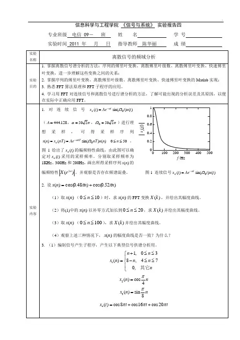
实验内容1.对连续信号)()sin()(0tutAetx taΩα-=(128.444=A,πα250=,πΩ250=)进行理想采样,可得采样序列50)()sin()()(0≤≤==-nnunTAenTxnx nTaΩα。
图1给出了)(txa的幅频特性曲线,由此图可以确定对)(txa采用的采样频率。
分别取采样频率为1KHz、300Hz和200Hz,画出所得采样序列)(nx的幅频特性)(ωj eX。
并观察是否存在频谱混叠。
图1 连续信号)()sin()(0tutAetx taΩα-=2. 设)52.0cos()48.0cos()(nnnxππ+=(1)取)(nx(100≤≤n)时,求)(nx的FFT变换)(kX,并绘出其幅度曲线。
(2)将(1)中的)(nx以补零方式加长到200≤≤n,求)(kX并绘出其幅度曲线。
(3)取)(nx(1000≤≤n),求)(kX并绘出其幅度曲线。
(4)观察上述三种情况下,)(nx的幅度曲线是否一致?为什么?3. (1)编制信号产生子程序,产生以下典型信号供谱分析用。
11,03()8,470,n nx n n nn+≤≤⎧⎪=-≤≤⎨⎪⎩其它2()cos4x n nπ=3()sin8x n nπ=4()cos8cos16cos20x t t t tπππ=++10.80.60.40.20100200300400500xa(jf)f /Hz(2)对信号1()x n ,2()x n ,3()x n 进行两次谱分析,FFT 的变换区间N 分别取8和16,观察两次的结果是否一致?为什么?(3)连续信号4()x n 的采样频率64s f Hz =,16,32,64N =。
信号与系统实验报告目录1. 内容概要 (2)1.1 研究背景 (3)1.2 研究目的 (4)1.3 研究意义 (4)2. 实验原理 (5)2.1 信号与系统基本概念 (7)2.2 信号的分类与表示 (8)2.3 系统的分类与表示 (9)2.4 信号与系统的运算法则 (11)3. 实验内容及步骤 (12)3.1 实验一 (13)3.1.1 实验目的 (14)3.1.2 实验仪器和设备 (15)3.1.4 实验数据记录与分析 (16)3.2 实验二 (16)3.2.1 实验目的 (17)3.2.2 实验仪器和设备 (18)3.2.3 实验步骤 (19)3.2.4 实验数据记录与分析 (19)3.3 实验三 (20)3.3.1 实验目的 (21)3.3.2 实验仪器和设备 (22)3.3.3 实验步骤 (23)3.3.4 实验数据记录与分析 (24)3.4 实验四 (26)3.4.1 实验目的 (27)3.4.2 实验仪器和设备 (27)3.4.4 实验数据记录与分析 (29)4. 结果与讨论 (29)4.1 实验结果汇总 (31)4.2 结果分析与讨论 (32)4.3 结果与理论知识的对比与验证 (33)1. 内容概要本实验报告旨在总结和回顾在信号与系统课程中所进行的实验内容,通过实践操作加深对理论知识的理解和应用能力。
实验涵盖了信号分析、信号处理方法以及系统响应等多个方面。
实验一:信号的基本特性与运算。
学生掌握了信号的表示方法,包括连续时间信号和离散时间信号,以及信号的基本运算规则,如加法、减法、乘法和除法。
实验二:信号的时间域分析。
在本实验中,学生学习了信号的波形变换、信号的卷积以及信号的频谱分析等基本概念和方法,利用MATLAB工具进行了实际的信号处理。
实验三:系统的时域分析。
学生了解了线性时不变系统的动态响应特性,包括零状态响应、阶跃响应以及脉冲响应,并学会了利用MATLAB进行系统响应的计算和分析。

合肥工业大学宣城校区《信号与系统》课程实验报告专业班级学生姓名《信号与系统》课程实验报告一实验名称一阶系统的阶跃响应姓名系院专业班级学号实验日期指导教师成绩一、实验目的1.熟悉一阶系统的无源和有源电路;2.研究一阶系统时间常数T的变化对系统性能的影响;3.研究一阶系统的零点对系统响应的影响。
二、实验原理1.无零点的一阶系统无零点一阶系统的有源和无源电路图如图2-1的(a)和(b)所示。
它们的传递函数均为:10.2s1G(s)=+(a) 有源(b) 无源图2-1 无零点一阶系统有源、无源电路图2.有零点的一阶系统(|Z|<|P|)图2-2的(a)和(b)分别为有零点一阶系统的有源和无源电路图,它们的传递函数为:10.2s1)0.2(sG(s)++=,⎪⎪⎪⎪⎭⎫⎝⎛++=S611S161G(s)(a) 有源(b) 无源图2-2 有零点(|Z|<|P|)一阶系统有源、无源电路图3.有零点的一阶系统(|Z|>|P|)图2-3的(a)和(b)分别为有零点一阶系统的有源和无源电路图,它们的传递函数为:1s10.1sG(s)=++(a) 有源(b) 无源图2-3 有零点(|Z|>|P|)一阶系统有源、无源电路图三、实验步骤1.打开THKSS-A/B/C/D/E型信号与系统实验箱,将实验模块SS02插入实验箱的固定孔中,利用该模块上的单元组成图2-1(a)(或(b))所示的一阶系统模拟电路。
2.实验线路检查无误后,打开实验箱右侧总电源开关。
3.将“阶跃信号发生器”的输出拨到“正输出”,按下“阶跃按键”按钮,调节电位器RP1,使之输出电压幅值为1V,并将“阶跃信号发生器”的“输出”端与电路的输入端“Ui”相连,电路的输出端“Uo”接到双踪示波器的输入端,然后用示波器观测系统的阶跃响应,并由曲线实测一阶系统的时间常数T。
4.再依次利用实验模块上相关的单元分别组成图2-2(a)(或(b))、2-3(a)(或(b))所示的一阶系统模拟电路,重复实验步骤3,观察并记录实验曲线。

信号与系统实验报告在现代科学与工程领域中,信号与系统是一个至关重要的研究方向。
信号与系统研究的是信号的产生、传输和处理,以及系统对信号的响应和影响。
在这个实验报告中,我们将讨论一些关于信号与系统实验的内容,以及实验结果的分析和讨论。
实验一:信号的采集与展示在这个实验中,我们学习了信号的采集与展示。
信号是通过传感器或其他仪器采集的电压或电流的变化,可以是连续的或离散的。
我们使用示波器和数据采集卡来采集信号,并在计算机上进行展示和分析。
实验二:线性时不变系统的特性线性时不变系统是信号与系统中的重要概念。
在这个实验中,我们通过观察系统对不同的输入信号作出的响应来研究系统的特性。
我们使用信号发生器产生不同的输入信号,并观察输出信号的变化。
通过比较输入信号和输出信号的频谱以及幅度响应,我们可以了解系统的频率响应和幅频特性。
实验三:系统的时域特性分析在这个实验中,我们将研究系统的时域特性。
我们使用了冲击信号和阶跃信号作为输入信号,观察输出信号的变化。
通过测量系统的冲击响应和阶跃响应,我们可以了解系统的单位冲激响应和单位阶跃响应。
实验四:卷积与系统的频域特性在这个实验中,我们学习了卷积的概念和系统的频域特性。
卷积是信号与系统中的重要运算,用于计算系统对输入信号的响应。
我们通过使用傅里叶变换来分析系统的频域特性,观察输入信号和输出信号的频谱变化。
实验五:信号的采样与重构在这个实验中,我们研究了信号的采样与重构技术。
信号的采样是将连续时间的信号转换为离散时间的过程,而信号的重构是将离散时间的信号恢复为连续时间的过程。
我们使用数据采集卡来对信号进行采样,并使用数字滤波器来进行信号的重构。
通过观察信号的采样和重构结果,我们可以了解采样率对信号质量的影响。
实验六:系统的稳定性与性能在这个实验中,我们研究了系统的稳定性与性能。
系统的稳定性是指系统对输入信号的响应是否有界,而系统的性能是指系统对不同频率信号的响应如何。
我们使用极坐标图和Nyquist图来分析系统的稳定性和性能,通过观察图形的变化来评估系统的性能。
信号与系统分析实验报告信号与系统分析实验报告引言:信号与系统分析是电子工程领域中的重要课程之一,通过实验可以更好地理解信号与系统的基本概念和原理。
本实验报告将对信号与系统分析实验进行详细的描述和分析。
实验一:信号的采集与重构在这个实验中,我们学习了信号的采集与重构。
首先,我们使用示波器采集了一个正弦信号,并通过数学方法计算出了信号的频率和幅值。
然后,我们使用数字信号处理器对采集到的信号进行重构,并与原始信号进行比较。
实验结果表明,重构后的信号与原始信号非常接近,证明了信号的采集与重构的有效性。
实验二:线性系统的时域响应本实验旨在研究线性系统的时域响应。
我们使用了一个线性系统,通过输入不同的信号,观察输出信号的变化。
实验结果显示,线性系统对于不同的输入信号有不同的响应,但都遵循线性叠加的原则。
通过分析输出信号与输入信号的关系,我们可以得出线性系统的传递函数,并进一步研究系统的稳定性和频率响应。
实验三:频域特性分析在这个实验中,我们研究了信号的频域特性。
通过使用傅里叶变换,我们将时域信号转换为频域信号,并观察信号的频谱。
实验结果显示,不同频率的信号在频域上有不同的分布特性。
我们还学习了滤波器的设计和应用,通过设计一个低通滤波器,我们成功地去除了高频噪声,并得到了干净的信号。
实验四:系统辨识本实验旨在研究系统的辨识方法。
我们使用了一组输入信号和对应的输出信号,通过数学建模的方法,推导出了系统的传递函数。
实验结果表明,通过系统辨识可以准确地描述系统的特性,并为系统的控制和优化提供了基础。
结论:通过本次实验,我们深入学习了信号与系统分析的基本概念和原理。
实验结果证明了信号的采集与重构的有效性,线性系统的时域响应的线性叠加原则,信号的频域特性和滤波器的设计方法,以及系统辨识的重要性。
这些知识和技能对于我们理解和应用信号与系统分析具有重要的意义。
通过实验的实际操作和分析,我们对信号与系统的理论有了更深入的理解,为我们今后的学习和研究打下了坚实的基础。
实验三常见信号的MATLAB表示及运算一、实验目的1. 熟悉常见信号的意义、特性及波形2. 学会使用MATLAB表示信号的方法并绘制信号波形3.掌握使用MATLAB进行信号基本运算的指令4.熟悉用MATLAB实现卷积积分的方法二、实验原理根据MA TLAB的数值计算功能和符号运算功能, 在MATLAB中, 信号有两种表示方法, 一种是用向量来表示, 另一种则是用符号运算的方法。
在采用适当的MATLAB语句表示出信号后, 就可以利用MATLAB中的绘图命令绘制出直观的信号波形了。
1.连续时间信号从严格意义上讲, MATLAB并不能处理连续信号。
在MATLAB中, 是用连续信号在等时间间隔点上的样值来近似表示的, 当取样时间间隔足够小时, 这些离散的样值就能较好地近似出连续信号。
在MATLAB中连续信号可用向量或符号运算功能来表示。
⑴向量表示法对于连续时间信号, 可以用两个行向量f和t来表示, 其中向量t是用形如的命令定义的时间范围向量, 其中, 为信号起始时间, 为终止时间, p为时间间隔。
向量f为连续信号在向量t所定义的时间点上的样值。
⑵符号运算表示法如果一个信号或函数可以用符号表达式来表示, 那么我们就可以用前面介绍的符号函数专用绘图命令ezplot()等函数来绘出信号的波形。
⑶常见信号的MATLAB表示单位阶跃信号单位阶跃信号的定义为:方法一: 调用Heaviside(t)函数首先定义函数Heaviside(t) 的m函数文件,该文件名应与函数名同名即Heaviside.m。
%定义函数文件,函数名为Heaviside,输入变量为x,输出变量为yfunction y= Heaviside(t)y=(t>0); %定义函数体, 即函数所执行指令%此处定义t>0时y=1,t<=0时y=0, 注意与实际的阶跃信号定义的区别。
方法二: 数值计算法在MATLAB中, 有一个专门用于表示单位阶跃信号的函数, 即stepfun( )函数, 它是用数值计算法表示的单位阶跃函数。
信号与系统的实验报告信号与系统的实验报告引言:信号与系统是电子工程、通信工程等领域中的重要基础学科,它研究的是信号的传输、处理和变换过程,以及系统对信号的响应和特性。
在本次实验中,我们将通过实际操作和数据分析,深入了解信号与系统的相关概念和实际应用。
实验一:信号的采集与重构在这个实验中,我们使用了示波器和函数发生器来采集和重构信号。
首先,我们通过函数发生器产生了一个正弦信号,并将其连接到示波器上进行观测。
通过调整函数发生器的频率和幅度,我们可以观察到信号的不同特性,比如频率、振幅和相位等。
然后,我们将示波器上的信号通过数据采集卡进行采集,并使用计算机软件对采集到的数据进行处理和重构。
通过对比原始信号和重构信号,我们可以验证信号的采集和重构过程是否准确。
实验二:信号的时域分析在这个实验中,我们使用了示波器和频谱分析仪来对信号进行时域分析。
首先,我们通过函数发生器产生了一个方波信号,并将其连接到示波器上进行观测。
通过调整函数发生器的频率和占空比,我们可以观察到方波信号的周期和占空比等特性。
然后,我们使用频谱分析仪对方波信号进行频谱分析,得到信号的频谱图。
通过分析频谱图,我们可以了解信号的频率成分和能量分布情况,进而对信号的特性进行深入研究。
实验三:系统的时域响应在这个实验中,我们使用了函数发生器、示波器和滤波器来研究系统的时域响应。
首先,我们通过函数发生器产生了一个正弦信号,并将其连接到滤波器上进行输入。
然后,我们通过示波器观测滤波器的输出信号,并记录下其时域波形。
通过改变滤波器的参数,比如截止频率和增益等,我们可以观察到系统对信号的响应和滤波效果。
通过对比输入信号和输出信号的波形,我们可以分析系统的时域特性和频率响应。
实验四:系统的频域响应在这个实验中,我们使用了函数发生器、示波器和频谱分析仪来研究系统的频域响应。
首先,我们通过函数发生器产生了一个正弦信号,并将其连接到系统中进行输入。
然后,我们通过示波器观测系统的输出信号,并记录下其时域波形。
实验五:基于Matlab的连续信号生成及时频域分析一、实验要求1、通过这次实验,学生应能掌握Matlab软件信号表示与系统分析的常用方法。
2、通过实验,学生应能够对连续信号与系统的时频域分析方法有更全面的认识。
二、实验内容一周期连续信号1)正弦信号:产生一个幅度为2,频率为4Hz,相位为π/6的正弦信号;2)周期方波:产生一个幅度为1,基频为3Hz,占空比为20%的周期方波。
非周期连续信号3)阶跃信号;4)指数信号:产生一个时间常数为10的指数信号;5)矩形脉冲信号:产生一个高度为1、宽度为3、延时为2s的矩形脉冲信号。
三、实验过程一1)t=0:0.001:1;ft1=2*sin(8*pi*t+pi/6);plot(t,ft1);2)t=0:0.001:2;ft1=square(6*pi*t,20);plot(t,ft1),axis([0,2,-1.5,1.5]);3)t=-2:0.001:2;y=(t>0);ft1=y;plot(t,ft1),axis([-2,2,-1,2]);4)t=0:0.001:30;ft1=exp(-1/10*t);plot(t,ft1),axis([0,30,0,1]);5)t=-2:0.001:6;ft1=rectpuls(t-2,3);plot(t,ft1),axis([-2,6,-0.5,1.5]);四、实验内容二1)信号的尺度变换、翻转、时移(平移)已知三角波f(t),用MATLAB画信号f(t)、f(2t)和f(2-2t) 波形,三角波波形自定。
2)信号的相加与相乘相加用算术运算符“+”实现,相乘用数组运算符“.*”实现。
已知信号x(t)=exp(-0.4*t),y(t)=2cos(2pi*t),画出信号x(t)+y(t)、x(t)*y(t)的波形。
3)离散序列的差分与求和、连续信号的微分与积分已知三角波f(t),画出其微分与积分的波形,三角波波形自定。
大连理工大学实验报告学院(系):电信专业:电子信息工程班级:姓名:学号:组: 实验时间:实验室:创新园C221 实验台: 指导教师签字:成绩:实验四:离散时间LIT 系统分析一、实验结果与分析1.试用MATLAB 命令求解以下离散时间系统的单位冲激响应。
(1)[][][][][]34121y n y n y n x n x n +-+-=+-(2)[][][][]5611022y n y n n x n +-+-= 解:(1)a =[3 4 1];b=[1 1]; n=0:30;impz(b,a,30),grid ontitle('系统单位冲激响应h(n)')(2)a=[2.5 6 10];b=[1]; n=0:30;impz(b,a,30),grid ontitle('系统单位冲激响应h(n)')2.已知某系统的单位冲激响应为[][][]{}7108nh n u n u n ⎛⎫=-- ⎪⎝⎭,试用MATLAB 求当激励信号为[][][]5x n u n u n =--时系统的零状态响应。
解:定义函数conv_m 如下:function [y,ny]=conv_m(x,nx,h,nh)ny1=nx(1)+nh(1);ny2=nx(length(x))+nh(length(h)); ny=[ny1:ny2]; y=conv(x,h) 主程序: nx=-1:6; nh=-2:12;x=heaviside(nx)- heaviside (nx-5);h=(7/8).^nh.*( heaviside (nh)- heaviside (nh-10)); [y,ny]=conv_m(x,nx,h,nh); subplot(311)stem(nx,x,'fill'),grid on xlabel('n'),title('x(n)') axis([-4 16 0 3]) subplot(312)stem(nh,h','fill'),grid on xlabel('n'),title('h(n)') axis([-4 16 0 3]) subplot(313)stem(ny,y,'fill'),grid onxlabel('n'),title('y(n)=x(n)*h(n)') axis([-4 16 0 3])3.试用MATLAB 画出下列因果系统的系统函数零极点分布图,并判断系统的稳定性。
《信号与系统》实验报告目录一、实验概述 (2)1. 实验目的 (2)2. 实验原理 (3)3. 实验设备与工具 (4)二、实验内容与步骤 (5)1. 实验一 (6)1.1 实验目的 (7)1.2 实验原理 (7)1.3 实验内容与步骤 (8)1.4 实验结果与分析 (9)2. 实验二 (10)2.1 实验目的 (12)2.2 实验原理 (12)2.3 实验内容与步骤 (13)2.4 实验结果与分析 (14)3. 实验三 (15)3.1 实验目的 (16)3.2 实验原理 (16)3.3 实验内容与步骤 (17)3.4 实验结果与分析 (19)4. 实验四 (20)4.1 实验目的 (20)4.2 实验原理 (21)4.3 实验内容与步骤 (22)4.4 实验结果与分析 (22)三、实验总结与体会 (24)1. 实验成果总结 (25)2. 实验中的问题与解决方法 (26)3. 对信号与系统课程的理解与认识 (27)4. 对未来学习与研究的展望 (28)一、实验概述本实验主要围绕信号与系统的相关知识展开,旨在帮助学生更好地理解信号与系统的基本概念、性质和应用。
通过本实验,学生将能够掌握信号与系统的基本操作,如傅里叶变换、拉普拉斯变换等,并能够运用这些方法分析和处理实际问题。
本实验还将培养学生的动手能力和团队协作能力,使学生能够在实际工程中灵活运用所学知识。
本实验共分为五个子实验,分别是:信号的基本属性测量、信号的频谱分析、信号的时域分析、信号的频域分析以及信号的采样与重构。
每个子实验都有明确的目标和要求,学生需要根据实验要求完成相应的实验内容,并撰写实验报告。
在实验过程中,学生将通过理论学习和实际操作相结合的方式,逐步深入了解信号与系统的知识体系,提高自己的综合素质。
1. 实验目的本次实验旨在通过实践操作,使学生深入理解信号与系统的基本原理和概念。
通过具体的实验操作和数据分析,掌握信号与系统分析的基本方法,提高解决实际问题的能力。
武汉大学教学实验报告
电子信息学院专业年月日实验名称指导教师
姓名年级学号成绩
(2)观察Gibbs 现象
分别取前10、20、30 和40 项有限级数来逼近奇对称方波,观察Gibbs 现象时得到的图如下
绘制周期信号的频谱
分析奇对称方波信号与偶对称三角信号的频谱,编制程序后画出图像如下所示(左上坐下分别为周期三角波及其频谱,右上右下为周期方波及其频谱)
2.实验操作过程
附件——matlab源文件
实验三
%周期三角信号的傅里叶级数
%author郑程耀
clear all;clc;
t=0:0.00001:0.04;
period=0.02;%周期
amplitude=1;%振幅
AC_coe=(4*amplitude)/(pi^2);%交流分量的系数
DC_coe=amplitude/2;%直流分量的系数
fre_w=(2*pi)/period;%圆频率
p=[1 2 5 100];
%t_z=0:0.01:t(end); %最简单的三角波
z=abs(sawtooth(t*(pi/period), 0.5)); %
figure
for ind_p=1:length(p)
y=DC_coe;
for k=1:p(ind_p)
y=y+DC_coe*cos((2*k-1)*fre_w*t)/(2*k-1)^2; end
subplot(2,2,ind_p)
plot(t,y)
hold on
plot(t,z,'r')
axis([0,0.04,-0.5,1.5]);
xlabel('time');
ylabel(strcat('前',num2str(p(ind_p)) ,'项有限级数')); end
实验四
%直接用公式计算各频率分量的振幅,并将他们画出来
%周期三角信号,方波信号的傅里叶级数
%author:郑程耀
clear all;clc;
period=0.02;%周期
t=0:0.00001:0.04;
N=15;
fre_n=1:2:2*N-1;
fre_n=[0 fre_n];
amplitude=1;%振幅
AC_coe=(4*amplitude)/(pi^2);%交流分量的系数
DC_coe=amplitude/2;%直流分量的系数
amplitude_w=DC_coe;
for k=1:length(fre_n)-1
amplitude_k=AC_coe/(2*k-1)^2;
amplitude_w=[amplitude_w amplitude_k];
end
figure
subplot(223)
stem(fre_n,amplitude_w,'*')
axis([-5 fre_n(end) 0 max(amplitude_w)*1.1])
title('三角波频谱')
xlabel('w')
ylabel('幅值')
%三角波波形
z=abs(sawtooth(t*(pi/period), 0.5)); %
subplot(221)
plot(t,z,'r')
title('三角波波形')
xlabel('time')
ylabel('amplitude')
%周期方波信号傅里叶级数
amplitude=6;%振幅
AC_coe=2*amplitude/pi ;%交流分量的系数
DC_coe=0;%直流分量的系数
amplitude_w=zeros(1,length(fre_n));
amplitude_w(1)=DC_coe;
for k=1:length(fre_n)-1
amplitude_k=AC_coe/(2*k-1);
amplitude_w(k+1)=amplitude_k;
end
subplot(224)
stem(fre_n,amplitude_w,'*')
axis([-5 fre_n(end) 0 max(amplitude_w)*1.1])
title('方波频谱')
xlabel('w')
ylabel('幅值')
%方波波形
subplot(222)
z_s=3*stepfun(t,0)-6*stepfun(t,0.01)+6*stepfun(t,0.02)-6*stepfun(t,0.03)+3*stepfun(t,0.04); plot(t,z_s)
title('方波波波形');
axis([0 0.04 -3.5 3.5])
xlabel('time')
ylabel('amplitude')。