flac3d5.0结构单元教程ppt课件
- 格式:ppt
- 大小:6.82 MB
- 文档页数:157


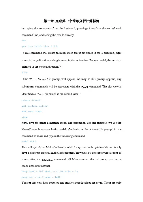
第二章完成第一个简单分析计算样例by typing the commands from the keyboard, pressing<Enter>at the end of each command line, and seeing the results directly.newgen zone brick size 6 8 8(This command will create an initial mesh that is six zones in the x-direction, eight zones in the y-direction and eight zones in the z-direction. For our model, the z-axis is oriented in the verticaldirection.)Plot(the Plot Base/0>prompt will appear. As long as this prompt appears, any subsequentcommands will be associated with the PLOT command. The plot view is identified as Base/0,which is the default view.)create Trenchadd surface yellowadd axes blackshowNow, give the zones a material model and properties. For this example, we use the Mohr-Coulombelastic-plastic model. Go back to the Flac3D>prompt in the command window andtype in thefollowing command:modelmohrThis will specify the Mohr-Coulomb model. Every zone in the grid could conceivably have adifferent material model and property. However, by not specifying a range of zonesafter the MODEL command, FLAC3D assumes that all zones are to be Mohr-Coulomb material.prop bulk = 1e8 shear = 0.3e8 fric = 35propcoh = 1e10 tens = 1e10You see that very high cohesion and tensile strength values are given. These areonlyinitial values that are used during the development of gravitational stresses within the body.In effect, we are forcing the body to behave elastically during the development of theinitial insitustress state.* This prevents any plastic yield during the initial loading phase of theanalysis.For this problem, loading is due to gravity. To apply gravity, use the commands setgrav 0, 0, -9.81ini dens = 1000In order to develop a gravitational body force, themass density must also be initialized. The INI command is used to initialize the mass density to1000 kg/m3 for all zones in the model.Next, the boundary conditions for the problem are set. At the Flac3D>prompt, type fix x range x -0.1 0.1fix x range x 5.9 6.1fix y range y -0.1 0.1fix y range y 7.9 8.1fix z range z -0.1 0.1With these commands, roller boundaries are placed on five sides of the model. The boundaries are “fixed” only in the specified direction (i.e., no displacement or velocity is allowed). The FIX commands perform the following functions.1. The gridpoints along the boundary planes at x = 0 and x = 6 are fixed in the x-direction. These two planes fall within the coordinate ranges specified by the range keywords for the first two FIX commands.2. The gridpoints along the boundary planes at y = 0 and y = 8 are fixed in the y-direction. These planes fall within the ranges specified for the third and fourth FIX commands.3. The gridpoints along the bottom boundary (z = 0) are fixed in the z-direction. This plane falls within the range for the fifth FIX command.We wish to monitor the change in the values of selected variables in the model during the calculational stepping. A HISTORY command can assist in helping us determinewhether a stable equilibrium solution or unstable collapse is occurring. We type the following commands:hist n = 5histunbalhistgpzdisp 4,4,8We choose to monitor the change in variables every five calculation steps. It is always a good idea to monitor the maximum unbalanced force in a model. If the unbalanced force approaches a very small value and displacement histories become constant, this indicates that an equilibrium state is reached.To allow gravitational stresses to develop within the body, we timestep the simulation to equilibrium.Here the SOLVE command is used to detect equilibrium automatically.setmech force=50solveWhen the unbalanced force falls below the limiting value (a limiting force of 50 N is specified with the SET command), the run will stop.* The plots are updated, since they are still visible on the screen. Shutting down the plots will cause the model to cycle faster.plothist 1hist 2The unbalanced force history approaches zero, andthe displacement history becomes constant; both are indicators that an equilibriumstate has beenreached.Note that each history is numbered sequentially from 1 as it is entered via the HIST command. Return to the Flac3D> prompt and typeprinthistfor a listing of the histories and their corresponding numbers.Plotcreat trenchadd contour dispadd axes blackshowclearaddbcontourszzadd axesplot create GravVplot set plane dip=90 dd=0 origin=3,4,0plot set rot 15 0 20plot set center 2.5 4.2 4.0plot add bound behindplot add bcontszz planeplot add axesplot showThis sequence will create a view, which we have called GravV, and make it the current view. We then set a plane for that view oriented at a dip angle of 90◦ (from the xy-plane, assuming that negative-z is “down”), a dip direction of 0◦(measured clockwise from the positive y-axis in the xy-plane) and with one point on the plane at (x = 3, y = 4, z = 0). We add a wire-frame boundary plotted behind the plane and a block contour plot of the vertical stress component, σzz, on the plane. Finally, the model axes are added. The block contour plot, as opposed to an interpolated contour plot, displays the value of the stress calculated at each zone centroid. The color of each zone corresponds directly to the zone-based stress.It is wise to save the initial state so that you can restore it at any time to perform parameter studies.savetrench.savWe can change the current view from GravV to Trench with the commandplot current TrenchNow we can excavate a trench in the soil. First, typepropcoh=1e3 tens=1e3This will set the cohesion and tensile strength for all zones to 1000 Pa. These valuesfor strength arehigh enough to prevent failure in our initial state (i.e., unexcavated), but you shouldalways checkfor possible failure in the initial state by performing a few calculation steps. Toexcavate the trench,entermodel null range x=2,4 y=2,6 z=5,10With a low cohesion and vertical unsupported trench walls, collapse should occur. Because wewant to examine this process realistically, the large-strain logic is specified. This isdone by typingset largeFor plotting purposes, we wish to see only the change in displacements from the trench excavation, and not from the previous gravitational loading, so we zero out the x-, y- and z-displacement components:inixdis=0 ydis=0 zdis=0We purposely set the cohesion low enough to result in failure, so we do not want to use the SOLVE command with a limit for out-of-balance force (which checks for equilibrium). Oursimulation willnever converge to the equilibrium state. Instead, we can step through the simulationprocess onetimestep at a time, and plot and print the results of the collapse as it occurs. This is thereal powerof the explicit method. The model is not required to converge to equilibrium at eachcalculationcycle because we never have to solve a set of linear algebraic equationssimultaneously, as is thecase for implicit codes, with which many engineers are familiar.we use the STEP command: step 2000第三章FLAC 3D基础知识gridpointzonehorizontal boundary stressstructural cables(tiebacks)model boundaryinternal boundaries(excavation)roller bottom boundaryNamed ObjectsMacro Object—Typically, such an object contains a long, complex string that may be used repeatedly in the model. The pre-processor compares a string of command tokens to the list of defined macros and replaces any matching macro object with its fully expanded contents.macro Pt0 ’p0 0 0 0’macro Pt1 ’p1 add 10 0 0’macro Pt2 ’p2 add 0 10 0’macro Pt3 ’p3 add 0 0 10’macroModel_Size ’size 4 5 6’macroBig_Brick ’zone brick Pt0 Pt1 Pt2 Pt3 Model_Size’.genBig_Brick.macro ’Pt0’ ’p0 15 15 15’genBig_BrickThis pre-processing has two effects:(1) macro objects may be nested (but not recursively); and(2) the macro object name is removed from the command string.Model Object—Model objects, such as ranges in space, groups of zones in a model, or plot views, can be given userdefined names. Those objects can then be referred to by their names.gen zone brick size 6 6 6group Tunnel range x 1 5 y 0 6 z 1 5modelmohr..modelnul range group Tunnel.The named range and the named group are two very different model objects. The range pertains toa specified volume of space (or range of values), whereas the group identifies acollection of finitedifference zones in the model.Sign ConventionsDIRECT STRESS —Positive stresses indicate tension; negative stresses indicate compression.第四章初级实体建模技术Grid generation is performed via the GENERATE command and associated keywords that both define the number of zones in a model and shape the grid to fit a specified problem region.The number of zones is specified by the size keyword.It is best to start with a grid that has few zones (say, 1000 to 1500) to perform simple test runs andmake refinements to the grid. Then, increase the number of zones to improve theaccuracy.Using actual coordinatesgen zone brick size 6,8,8 p0 -10, -10, -20 &p1 10, -10, -20 &p2 -10, 10, -20 &p3 -10, -10, 0plot surfOnly four corners are required to define a parallelepiped-shaped mesh. More corners can be specifiedto define an irregular surface. Example 2.14 shows how to make a sloping surface atthe top of themesh.gen zone brick size 6,8,8 p0 -10, -10, -20 &p1 10, -10, -20 p2 -10, 10, -20 &p3 -10, -10, 0 p4 10, 10, -20 &p5 -10, 10, 10 p6 10, -10, 0 &p7 10, 10, 10plot surfIn the tutorial example, we noted that the boundaries of the model were influencing the results (see Figure 2.6). The boundary must be placed far enough away from the excavation to reduce these effects. A gradually graded mesh can be created in FLAC3D to move the model boundaries farther out without significantly increasingthe number of zones. For example, the command GEN zone radbrick creates a radially graded mesh around a brick-shaped mesh. The command in Example 2.15 creates a 3 ×5 ×5 zone brick-shaped mesh surrounded by a 7-zone radially graded mesh.gen zone radbrick&p0 (0,0,0) p1 (10,0,0) p2 (0,10,0) p3 (0,0,10) &size 3,5,5,7 &ratio 1,1,1,1.5 &dim 1 4 2 fillplot surfThe x,y,z coordinate system in FLAC3D is always right-handed and, as a default, the z-axis is drawn in the vertical direction on the screen. In Example 2.14 we assumed the z-axis was pointing in the vertical direction. However, we do not have to interpret the z-axis to mean the up direction. For Example 2.15, we will assume that the y-axis is the vertical direction. As long as we define the model in a right-handed system, we can create the grid in any direction we desire.The size keyword, as used in Example 2.15, specifies the number of zones in the brick and the number radially surrounding the brick (see Figure 2.11). The keyword ratio is given to manipulate the grid spacing. The four values that follow ratio are geometric ratios between successive zone sizes. The first three values are ratios for the zones in the brick, and the fourth value is the ratio for the zones surrounding the brick. In Example 2.15 above, the ratio is 1.0 for the brick zones and1.5 for the zones surrounding the brick. This causes each successive ring of zones surrounding the brick to be 1.5 times larger in the radial direction. The dim keyword defines the dimensions of the brick region (i.e., 1 m ×4 m ×2 m). The fill keyword fills the brick region with zones. If fill is omitted, no zones will be generated within the brick region.Notice that size, ratio and dim all refer to local axes as defined by p0, p1, p2, p3 in Figure 2.11, not to the global x,y,z-axes.Creating a model by reflecting elements on planes of symmetrygen zone radbrick&p0 (0,0,0) p1 (10,0,0) p2 (0,10,0) p3 (0,0,10) &size 3,5,5,7 &ratio 1,1,1,1.5 &dim 1 4 2 fillgen zone reflect dip 0 dd 90gen zone reflect dip 90 dd 90plot surfdip 为倾角的意思,其值大小为面与xy面所夹的倾角,dd为倾向,其值大小为面的法线在xy平面上的投影与y轴的夹角。


Flac3D5.0教程第⼆章完成第⼀个简单分析计算样例by typing the commands from the keyboard, pressingat the end of each command line, and seeing the results directly.newgen zone brick size 6 8 8(This command will create an initial mesh that is six zones in the x-direction, eight zones in the y-direction and eight zones in the z-direction. For our model, the z-axis is oriented in the verticaldirection.)Plot(the Plot Base/0>prompt will appear. As long as this prompt appears, any subsequentcommands will be associated with the PLOT command. The plot view is identified as Base/0,which is the default view.)create Trenchadd surface yellowadd axes blackshowNow, give the zones a material model and properties. For this example, we use the Mohr-Coulombelastic-plastic model. Go back to the Flac3D>prompt in the command window andtype in thefollowing command:modelmohrThis will specify the Mohr-Coulomb model. Every zone in the grid could conceivably have adifferent material model and property. However, by not specifying a range of zonesafter the MODEL command, FLAC3D assumes that all zones are to be Mohr-Coulomb material.prop bulk = 1e8 shear = 0.3e8 fric = 35propcoh = 1e10 tens = 1e10You see that very high cohesion and tensile strength values are given. These areonlyinitial values that are used during the development of gravitational stresses within the body.In effect, we are forcing the body to behave elastically during the development of theinitial insitustress state.* This prevents any plastic yield during the initial loading phase of theanalysis.For this problem, loading is due to gravity. To apply gravity, use the commands setgrav 0, 0, -9.81ini dens = 1000In order to develop a gravitational body force, themass density must also be initialized. The INI command is used to initialize the mass density to1000 kg/m3 for all zones in the model.Next, the boundary conditions for the problem are set. At the Flac3D>prompt, type fix x range x -0.1 0.1fix x range x 5.9 6.1fix y range y -0.1 0.1fix y range y 7.9 8.1fix z range z -0.1 0.1With these commands, roller boundaries are placed on five sides of the model. The boundaries are “fixed” only in the specified direction (i.e., no displacement or velocity is allowed). The FIX commands perform the following functions.1. The gridpoints along the boundary planes at x = 0 and x = 6 are fixed in the x-direction. These two planes fall within the coordinate ranges specified by the range keywords for the first two FIX commands.2. The gridpoints along the boundary planes at y = 0 and y = 8 are fixed in the y-direction. These planes fall within the ranges specified for the third and fourth FIX commands.3. The gridpoints along the bottom boundary (z = 0) are fixed in the z-direction. This plane falls within the range for the fifth FIX command.We wish to monitor the change in the values of selected variables in the model during the calculational stepping. A HISTORY command can assist in helping us determinewhether a stable equilibrium solution or unstable collapse is occurring. We type the following commands:hist n = 5histunbalhistgpzdisp 4,4,8We choose to monitor the change in variables every five calculation steps. It is always a good idea to monitor the maximum unbalanced force in a model. If the unbalanced force approaches a very small value and displacement histories become constant, this indicates that an equilibrium state is reached.To allow gravitational stresses to develop within the body, we timestep the simulation to equilibrium.Here the SOLVE command is used to detect equilibrium automatically.setmech force=50solveWhen the unbalanced force falls below the limiting value (a limiting force of 50 N is specified with the SET command), the run will stop.* The plots are updated, since they are still visible on the screen. Shutting down the plots will cause the model to cycle faster.plothist 1hist 2The unbalanced force history approaches zero, andthe displacement history becomes constant; both are indicators that an equilibriumstate has beenreached.Note that each history is numbered sequentially from 1 as it is entered via the HIST command. Return to the Flac3D> prompt and typeprinthistfor a listing of the histories and their corresponding numbers.Plotcreat trenchadd contour dispadd axes blackshowclearaddbcontourszzadd axesplot create GravVplot set plane dip=90 dd=0 origin=3,4,0plot set rot 15 0 20plot set center 2.5 4.2 4.0plot add bound behindplot add bcontszz planeplot add axesplot showThis sequence will create a view, which we have called GravV, and make it the current view. We then set a plane for that view oriented at a dip angle of 90? (from the xy-plane, assuming that negative-z is “down”), a dip direction of 0?(measured clockwise from the positive y-axis in the xy-plane) and with one point on the plane at (x = 3, y = 4, z = 0). We add a wire-frame boundary plotted behind the plane and a block contour plot of the vertical stress component, σzz, on the plane. Finally, the model axes are added. The block contour plot, as opposed to an interpolated contour plot, displays the value of the stress calculated at each zone centroid. The color of each zone corresponds directly to the zone-based stress.It is wise to save the initial state so that you can restore it at any time to perform parameter studies.savetrench.savWe can change the current view from GravV to Trench with the commandplot current TrenchNow we can excavate a trench in the soil. First, typepropcoh=1e3 tens=1e3This will set the cohesion and tensile strength for all zones to 1000 Pa. These valuesfor strength arehigh enough to prevent failure in our initial state (i.e., unexcavated), but you shouldalways checkfor possible failure in the initial state by performing a few calculation steps. Toexcavate the trench,entermodel null range x=2,4 y=2,6 z=5,10With a low cohesion and vertical unsupported trench walls, collapse should occur. Because wewant to examine this process realistically, the large-strain logic is specified. This isdone by typingset largeFor plotting purposes, we wish to see only the change in displacements from the trench excavation, and not from the previous gravitational loading, so we zero out the x-, y- and z-displacement components:inixdis=0 ydis=0 zdis=0We purposely set the cohesion low enough to result in failure, so we do not want to use the SOLVE command with a limit for out-of-balance force (which checks for equilibrium). Oursimulation willnever converge to the equilibrium state. Instead, we can step through the simulationprocess onetimestep at a time, and plot and print the results of the collapse as it occurs. This is thereal powerof the explicit method. The model is not required to converge to equilibrium at eachcalculationcycle because we never have to solve a set of linear algebraic equationssimultaneously, as is thecase for implicit codes, with which many engineers are familiar.we use the STEP command: step 2000第三章FLAC 3D基础知识gridpointzonehorizontal boundary stressstructural cables(tiebacks)model boundaryinternal boundaries(excavation)roller bottom boundaryNamed ObjectsMacro Object—Typically, such an object contains a long, complex string that may be used repeatedly in the model. The pre-processor compares a string of command tokens to the list of defined macros and replaces any matching macro object with its fully expanded contents.macro Pt0 ’p0 0 0 0’macro Pt1 ’p1 add 10 0 0’macro Pt2 ’p2 add 0 10 0’macro Pt3 ’p3 add 0 0 10’macroModel_Size ’size 4 5 6’macroBig_Brick ’zone brick Pt0 Pt1 Pt2 Pt3 Model_Size’.genBig_Brick.macro ’Pt0’ ’p0 15 15 15’genBig_BrickThis pre-processing has two effects:(1) macro objects may be nested (but not recursively); and(2) the macro object name is removed from the command string.Model Object—Model objects, such as ranges in space, groups of zones in a model, or plot views, can be given userdefined names. Those objects can then be referred to by their names.gen zone brick size 6 6 6group Tunnel range x 1 5 y 0 6 z 1 5modelmohr..modelnul range group Tunnel.The named range and the named group are two very different model objects. The range pertains toa specified volume of space (or range of values), whereas the group identifies acollection of finitedifference zones in the model.Sign ConventionsDIRECT STRESS —Positive stresses indicate tension; negative stresses indicate compression.第四章初级实体建模技术Grid generation is performed via the GENERATE command and associated keywords that both define the number of zones in a model and shape the grid to fit a specified problem region.The number of zones is specified by the size keyword.It is best to start with a grid that has few zones (say, 1000 to 1500) to perform simple test runs andmake refinements to the grid. Then, increase the number of zones to improve theaccuracy.Using actual coordinatesgen zone brick size 6,8,8 p0 -10, -10, -20 &p1 10, -10, -20 &p2 -10, 10, -20 &p3 -10, -10, 0plot surfOnly four corners are required to define a parallelepiped-shaped mesh. More corners can be specifiedto define an irregular surface. Example 2.14 shows how to make a sloping surface atthe top of themesh.gen zone brick size 6,8,8 p0 -10, -10, -20 &p1 10, -10, -20 p2 -10, 10, -20 &p3 -10, -10, 0 p4 10, 10, -20 &p5 -10, 10, 10 p6 10, -10, 0 &p7 10, 10, 10plot surfIn the tutorial example, we noted that the boundaries of the model were influencing the results (see Figure 2.6). The boundary must be placed far enough away from the excavation to reduce these effects. A gradually graded mesh can be created in FLAC3D to move the model boundaries farther out without significantly increasingthe number of zones. For example, the command GEN zone radbrick creates a radially graded mesh around a brick-shaped mesh. The command in Example 2.15 creates a 3 ×5 ×5 zone brick-shaped mesh surrounded by a 7-zone radially graded mesh.gen zone radbrick&p0 (0,0,0) p1 (10,0,0) p2 (0,10,0) p3 (0,0,10) &size 3,5,5,7 &ratio 1,1,1,1.5 &dim 1 4 2 fillplot surfThe x,y,z coordinate system in FLAC3D is always right-handed and, as a default, the z-axis is drawn in the vertical direction on the screen. In Example 2.14 we assumed the z-axis was pointing in the vertical direction. However, we do not have to interpret the z-axis to mean the up direction. For Example 2.15, we will assume that the y-axis is the vertical direction. As long as we define the model in a right-handed system, we can create the grid in any direction we desire.The size keyword, as used in Example 2.15, specifies the number of zones in the brick and the number radially surrounding the brick (see Figure 2.11). The keyword ratio is given to manipulate the grid spacing. The four values that follow ratio are geometric ratios between successive zone sizes. The first three values are ratios for the zones in the brick, and the fourth value is the ratio for the zones surrounding the brick. In Example 2.15 above, the ratio is 1.0 for the brick zones and1.5 for the zones surrounding the brick. This causes each successive ring of zones surrounding the brick to be 1.5 times larger in the radial direction. The dim keyword defines the dimensions of the brick region (i.e., 1 m ×4 m ×2 m). The fill keyword fills the brick region with zones. If fill is omitted, no zones will be generated within the brick region.Notice that size, ratio and dim all refer to local axes as defined by p0, p1, p2, p3 in Figure 2.11, not to the global x,y,z-axes.Creating a model by reflecting elements on planes of symmetrygen zone radbrick&p0 (0,0,0) p1 (10,0,0) p2 (0,10,0) p3 (0,0,10) &size 3,5,5,7 &ratio 1,1,1,1.5 &dim 1 4 2 fillgen zone reflect dip 0 dd 90gen zone reflect dip 90 dd 90plot surfdip 为倾⾓的意思,其值⼤⼩为⾯与xy⾯所夹的倾⾓,dd为倾向,其值⼤⼩为⾯的法线在xy平⾯上的投影与y轴的夹⾓。
FL AC3 D5. 0 模型及输入参数说明模型参数代码可参考ma nua I中各个章节的comma nd命令及说明,注意单位。
用prop赋值。
各向同性弹性模型模型修正剑桥模型经典粘弹性模型1.1.14二分幕律模型5 mviscosity Maxwell 动力粘度,朮碎盐变形模型1.2模型适用说明遍布节理模型适用于Mohr-Coulomb材料来明确显示力在各个方向上的差异性。
双线性软化应变遍布节理模型综合了软化应变Mohr-Coulomb模型和遍布节理模型,这种模型包含面向矩阵和遍布节理的一个双线性断裂点集。
改进的Cam-clay 模型反映了形变度和抗破坏能力对体积变化的影响。
Mohr-Coulomb模型最适用于一般工程研究,同时,Mohr-Coulomb的内聚力和摩擦角参数相对于地质工程材料的其它属性,更容易获得。
软化应变和遍布节理塑性模型实际上是Mohr-Coulomb模型的变形,这些模型如果在附加材料参数的值较高时将得出与Mohr-Coulomb模型同样的结果。
Druck-Prager模型是一个相对于Mohr-Coulomb 模型的破坏标准的简化体,但是它一般不适于用来描述地质工程材料的破坏情况。
它主要是用来把FLAC3D与其它一些有Druck-Prager模型但却没有Mohr-Coulomb模型的数学软件作比较。
在摩擦力为零的时候请注意,此时Mohr-Coulomb模型退化为Tresca模型,而Druck-Prager 模型退化为Von Mises模型。
Druck-Prager模型和Mohr-Coulomb模型是计算起来效率最高的塑性模型,而其它的塑性模型在计算时却需要更多的内存和额外的时间。
例如,塑性应变不能在Mohr-Coulomb模型中直接计算出来(参见附录G)。
如果需要计算塑性应变,则必需要用应变软化模型。
这种模型主要是用于破坏后的情况对工程影响重大的工程活动中,如弯曲柱、开采塌落或回填研究。