并联式涡轮冲压组合发动机安装性能数值模拟 (1)
- 格式:pdf
- 大小:314.57 KB
- 文档页数:7

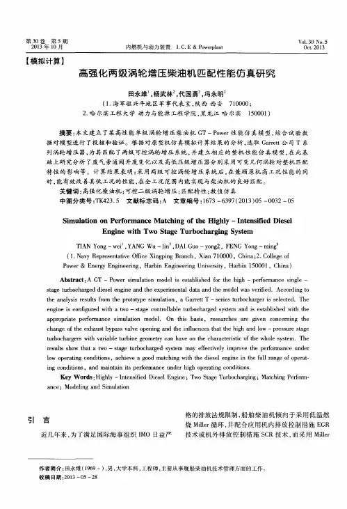

涡轮增压柴油机平均值模型建模及模型校核方法研究共3篇涡轮增压柴油机平均值模型建模及模型校核方法研究1涡轮增压柴油机平均值模型建模及模型校核方法研究涡轮增压柴油机是现代车辆中常用的动力来源。
与传统的机械增压相比,涡轮增压可以更加有效地提高发动机的动力性能和燃烧效率,同时降低排放物的排放。
因此,建立涡轮增压柴油机的平均值模型及其校核方法具有重要的理论意义和实际应用价值。
本文以6缸涡轮增压柴油机为例,建立了其平均值模型。
根据热力学和动力学原理,将发动机分为进气系统、燃油系统、排气系统和运动系统四个部分,分别建立各自的数学模型。
其中,进气系统模型涵盖了进气道、空气滤清器、进气门等组成部分,并考虑了进气道干燥器和冷却器的影响。
燃油系统模型考虑了高压油泵、喷油嘴和燃油储油器等组成部分,并引入了燃油喷射策略模型。
排气系统模型包括了排气歧管、涡轮增压器、废气再循环系统等组成部分,并考虑了废气再循环对氧气含量的影响。
运动系统模型涉及了曲轴、连杆、活塞等组成部分,并引入了气缸压力和扭矩输出模型。
为了验证所建立的平均值模型的准确性和可用性,本文还提出了一种基于均衡点分析法的模型校核方法。
通过采集实际发动机的运行数据,计算出其运行参数和燃烧特性,并与模型预测结果进行比较。
根据比较结果,对模型的各项参数进行进行优化和修正,以达到更好的预测效果。
实验结果表明,所建立的平均值模型和校核方法能够较为准确地预测发动机的运行特性和性能参数,包括燃油消耗、排放物排放、空气流量等,且具有较好的通用性和可拓展性。
此外,模型校核方法也能够有效地提高模型的精度和稳定性,为涡轮增压柴油机的优化和控制提供了基础和支持。
总之,涡轮增压柴油机平均值模型建模及模型校核方法的研究对于提高车辆动力性能和减少环境污染具有重要的意义和价值。
未来研究可以进一步深入探讨模型的可靠性和灵敏度,以及在实际应用中的优化和改进方法本文提出了一种涡轮增压柴油机的平均值模型及其校核方法,并通过实验验证了其可用性和准确性。

涡轮增压柴油机平均值模型建模及模型校核方法研究
涡轮增压柴油机的平均值模型建模及模型校核是研究如何对涡轮增压柴油机进行数学建模,并校核模型的有效性和准确性的方法研究。
涡轮增压柴油机是一种通过涡轮增压系统提高进气量和气缸充填效率的内燃机。
平均值模型建模是通过对柴油机的各个子系统进行建模和描述,以推导出模型的数学表达式和方程。
这些子系统包括气缸、进气系统、燃油系统、排气系统等等。
建模过程需要考虑模型的物理原理、参数表达和各个子系统之间的相互作用关系。
模型校核是指通过与实际测试数据对比,验证模型的准确性和有效性。
校核方法可以采用计算机模拟和实验验证相结合的方式。
计算机模拟可以使用数值计算方法,将建立的模型进行数值求解,并与实际测试数据进行对比。
实验验证可以通过在实际涡轮增压柴油机上进行测试,获取实际数据,并与模型的预测结果进行比较。
在进行模型校核时,需要考虑多个因素,如不同工况下的模型准确性、模型可靠性和模型复杂度等。
模型校核的目标是不断改进和优化模型,使其能够更好地预测和描述涡轮增压柴油机的工作性能和特性。
总结起来,涡轮增压柴油机平均值模型建模及模型校核方法研究是对涡轮增压柴油机进行数学建模,并通过与实际测试数据
对比验证模型准确性和有效性的研究。
它对于涡轮增压柴油机的设计、优化和性能预测具有重要的意义。
Dual-Mode Scramjet Performance Model for TBCCSimulationEric J. Gamble*, Dan Haid†, Sal D’Alessandro‡, and Rich DeFrancesco§SPIRITECH Advanced Products, Inc, Tequesta, FloridaA Turbine-Based Combined Cycle (TBCC) dynamic simulation model is being developedto demonstrate all modes of operation, including mode transition, for a turbine-based combined cycle propulsion system. The High Mach Transient Engine Cycle Code (HiTECC)is a highly integrated tool comprised of modules for modeling each of the TBCC systems whose interactions and controllability affect the TBCC propulsion system thrust and operability during its modes of operation. By structuring the simulation modeling tools around the major TBCC functional modes of operation (Dry Turbojet, Afterburning Turbojet, Transition, and Dual Mode Scramjet) the TBCC mode transition and all necessary intermediate events over its entire mission may be developed, modeled, and validated. The reported work details the development of the gas turbine and dual-mode scramjet performance models conducted in the first year of a multiyear effort to develop a dynamic TBCC simulation model. Once completed, this model will significantly extend the state-of-the-art for all TBCC modes of operation by providing a numerical simulation of the systems, interactions, and transient responses affecting the ability of the propulsion system to transition from turbine-based to ramjet/scramjet-based propulsion while maintaining constant thrust.I.Nomenclaturea speed of sound (ft/s)A area(ft2)AOA angle of attackc velocity(ft/s)c p specific heat (btu/lbm/°R)C s stream thrust coefficientC fg thrust coefficientDH change in enthalpy (btu/lbm)e specificenergyerr systemerrorf frequency(Hz)F force(lbf)FAR Fuel-AirRatioh enthalpy (btu/lbm) or height (ft) I moment of inertiaK coefficientLoss component loss coefficient, ψ− ψ’ M MachnumberN shaft speed (RPM) or time steps PR pressureratioP pressure(psia)q heat flux (btu/ft2/s)R radius(ft) Re Reynoldsnumbert time (sec)T temperature (°R)TFF turbine flow function, w √T t / P tu speed (ft/s)v velocity(ft/s)V volume(ft3)w mass flow (lbm/s)W workx distance(ft)α dampingcoefficientχmass fraction or normalized distanceδ boundarylayerthicknessδ* displacementthicknessφflow coefficient or equivalence ratioγspecific heat ratioη efficiencyθangle (°), momentum thickness (ft), combustion parameter ρ density(lbm/ft3)τnon-dimensional temperature riseψ workcoefficientψ’ pressure coefficient* Vice President, SPIRITECH Advanced Products, Inc., member AIAA† Aerodynamic Engineer, SPIRITECH Advanced Products, Inc., member AIAA‡ Structural Engineer, SPIRITECH Advanced Products, Inc., non-member AIAA§ President, SPIRITECH Advanced Products, Inc., member AIAAAIAA-2009-5298TSubscripts0 freestream conditions 1 component inlet 2 component exit atm atmospheric BL boundary layer bleed bleedc calculated value comb combustion corr corrected to component inlet CLM component level model des design value eff effective f fuelg guess value H high-speed flow pathi spatial index loss loss L low-speed flow path, or length map map value MB moving boundary ML component minimum loss n temporal index scale map scale factor sep separation std standard day value s static conditions t total conditions tip blade tip visc viscous wall wall z axial directionSuperscripts ‘ ideal* sonicII. IntroductionHE need for the National Aeronautics and Space Administration (NASA) Aeronautics Research Mission Directorate (ARMD) Hypersonic Project is based on the fact that all access to earth or planetary orbit, and all entry into earth’s atmosphere or any heavenly body with an atmosphere from orbit (or super orbital velocities) require flight through the hypersonic regime. The hypersonic flight regime often proves to be the design driver for most of the vehicle’s systems, subsystems, and components. If the United States wishes to continue to advance its capabilities for space access, entry, and high-speed flight within any atmosphere, improved understanding of the hypersonic flight regime and development of improved technologies to withstand and/or take advantage of this environment are required.A critical element of NASA’s hypersonics research is the development of combined cycle propulsion systems, including rocket-based combined cycles (RBCC) and turbine-based combined cycles (TBCC). Based on the Next Generation Launch Technology (NGLT), TBCC, Two Stage to Orbit (TSTO), National AeroSpace Plane (NASP), and High Speed Propulsion Assessment (HiSPA) studies, a turbofan and ramjet variable cycle engine is best suited to satisfy the access-to-space mission requirements by maximizing thrust-to-weight ratio while minimizing frontal area and maintaining high performance and operability over a wide operating range. The TBCC Dynamic Simulation Model Development Program discussed in this paper advances the technology readiness level of TBCC systems by developing the simulation and controls software to model all modes of operation over its mission, including mode transition from gas turbine to dual-mode scramjet propulsion, a requirement before controlled wind tunnel testing or flight testing can be accomplished through this region of operation. Within this program, modeling tools are being developed from fundamental physics and are being integrated into a comprehensive dynamic simulation tool to determine the transient performance, providing actual event durations to properly configure the propulsion system control logic. Work accomplished to date includes the development of the gas turbine and dual-mode scramjet propulsion systems.III. Technical DiscussionA. Propulsion Model OrganizationThe TBCC propulsion system is divided into four subsystems. These are the Inlet, Gas Turbine, Dual Mode Scramjet (DMSJ), and Nozzle. Each of these subsystems is broken down further into components (i.e. the gas turbine contains a compressor, combustor, turbine, etc.). Figure 1 illustrates the organization of the High Mach Transient Engine Cycle Code (HiTECC) that is being developed to simulate a TBCC propulsion system. The Component Level of HiTECC contains the models of physical processes in the TBCC System. These models fall into one of two categories. The first includes routines that utilize performance maps where a number of dependentparameters are defined as a function of a number of independent parameters, usually in the form of look-up tables. These maps are typically applied when component performance can be accurately determined from a small number of independent variables and a significant improvement in computational performance can be achieved over more detailed models. Typical applications include compressors and turbines. The second category includes routines based on conservation models. These are physical models that balance the continuity, momentum, and energy equations across a component.ComponentSub ‐System System HiTECC TBCC SimulatorPropulsionThermal ManagementHydraulics ControlInlet Gas Turbine DMSJ NozzleCompressorCombustorTurbineAfterburnerExternal Low ‐Speed High ‐Speed Isolator CombustorLow ‐SpeedHigh ‐SpeedFigure 1. HiTECC TBCC Simulator Organization.B. Gas Model SelectionIt is well established that real gas effects significantly impact performance at the high Mach number and temperatures encountered in Scramjet engines 1. Unfortunately, real gas models require significantly more computational time than the simple calorically perfect ideal 2 and thermally perfect models. A study, summarized below, was conducted to identify regions where these simpler, less computationally intensive models could be applied.Static-to-total temperature and pressure ratios were predicted with calorically perfect (ideal), thermally perfect, and real gas assumptions as a function of Mach number for total temperatures ranging from 1000°R to 5000°R. The real gas calculations are based on a minimization-of-free-energy method conducted with NASA’s Chemical Equilibrium with Applications (CEA) code 3. At a given total temperature (enthalpy) and static pressure, static enthalpy is determined from the adiabatic energy equation over a range of velocities. The static temperature, speed of sound, and entropy are predicted from the static enthalpy and static pressure with the CEA code. The static temperature and speed of sound are used to generate the real gas static-to-total temperature ratio versus Mach number. The total pressure for the real gas static-to-total pressure ratio is determined from the entropy and total enthalpy with the CEA Code. The results, shown normalized by the results for calorically perfect gas in Figure 2, illustrate the errors associated with calorically perfect and thermally perfect gas assumptions with respect to real gas predictions. The error in temperature and pressure for the ideal gas assumption is small at 1000°R but increases to over 5% at 2000°R and Mach numbers greater than one. The error in temperature and pressure for thermally perfect assumption is small for total temperatures less than 3000°R. At higher temperatures, however, the error can become quite large due to dissociation.The inlet was identified as a prime candidate for the simpler gas models. Figure 3 shows the predicted total temperature of the flow entering the inlet for the three gas models. Snyder et al.4 determined that mode transition would occur near Mach 4 for an X-43B type vehicle. For transition Mach numbers near 4 and dynamic pressures greater than 1100 psf, mode transition will occur in the isothermal portion of the lower stratosphere where the ambient temperature is 390°R. The total temperatures from this plot can be used along with Figure 2 to obtain variations (error) from real gas behavior of the simpler models. The thermally perfect gas model provides reasonable accuracy (<2% error) up to flight Mach numbers of 7. The ideal gas model provides reasonable accuracy (<2% error) up to flight Mach numbers of 1. Since the maximum vehicle flight Mach number is 7, the thermally perfect gas model is used for supersonic flow, and the ideal gas model is used for transonic and subsonic flows.Mach Number()()id ea l T S T S T /T T /TMach Num ber()()ide alT S T S P /P P /P Figure 2. Comparison of Predicted Temperature and Pressure for Thermally Perfect and Ideal Gas versus Real Gas Chemical Equilibrium with Application (CEA) Calculations.010002000300040005000600070008000900010000024681012T t ,0Mach NumberIdeal Gas ( Thermally & Calorically Perfect)Thermally Perfect, Calorically ImperfectReal Gas ( Thermally & Calorically Imperfect)T s,atm = 390 °RError for Thermally Perfect Gas assumption less than 2% for MN < 7Error for Ideal Gasassumption less than 2% for MN < 3.4Figure 3. Freestream Total Temperature for Calorically Perfect Ideal, Thermally Perfect, and Real Gas Chemical Equilibrium with Application (CEA) Calculations.C. Propulsion Subsystem Modeling Inlet ModelFor this paper, the HiTECC simulation considers the Combined Cycle Engine Large scale Inlet for Mode Transition (CCE-L-IMX)5 as an inlet model. The CCE-L-IMX is a hardware model being fabricated to study mode transition in the NASA Glenn Research Center 10x10 supersonic wind tunnel. The inlet subsystem of HiTECC is made up of three models as shown in Figure 4. Low-order non-linear models were selected for their ability to simulate large flow perturbations and geometry changes relatively quickly and robustly. The first model is for external compression and is applied from the leading edge of the vehicle to the leading edge of the two inlet cowls. The second model is for supersonic internal compression and is applied from the leading edge of the low-speed cowl to the throat of the low-speed gas path and from the leading edge of the high-speed cowl to the isolator entrance in the high-speed gas path. These first two models are steady–state since it is expected that the response time of the supersonic streams will be relatively instantaneous compared to the other systems in the TBCC. The third model is for unsteady subsonic flow and is applied from the inlet throat to the engine face in the low-speed gas path.2L1.4L (Throat)1.0L1.0H2.0HExternalSupersonic InternalSubsonic InternalFigure 4. TBCC Inlet Model Overview.The external flow field is determined using inviscid, thermally perfect oblique-shock theory 2 as shown in Figure 5. The analytical method is similar to that used in the NASA Large Perturbation Inlet model (LAPIN)6. The flow-field is set up for three-shocks, two from the ramp and one from the low-speed flow path cowl lip extending into the high-speed flow path. Additional shocks (or expansion waves) can be added if required. The boundary layer, predicted by NASA’s PCBLYR code 7, is superimposed over the inviscid solution to improve predicted inlet mass flow capture and compression in the internal portion of the inlet.θ1θ2θ3HP atm T atm M 0Pt0T t0P s0.1T s0.1M 0.1P s0.2T s0.2M 0.2P s0.3T s0.3M 0.3AOA θ3LBoundary Layers Superimposed on Flow FieldFigure 5. Inlet Subsystem External Flow Field Calculation.The supersonic internal compression model is used in the regions defined from the leading edge of the low-speed cowl to the throat of the low-speed gas path and from the leading edge of the high-speed cowl to the isolator entrance in the high-speed gas path, as shown in Figure 6. This model uses thermally perfect one-dimensional steady-state compressible flow through a variable-area control volume with accommodations for viscosity, boundary layer bleed flow, and an oblique shock off the cowl lip.δ*: BLDisplacement from Blayer.exeStation 0.21L1.1L1.4LFigure 6. Regions Simulated Using Supersonic Internal Compression Analysis.P s1.1, T s1.1, M 1.1Thermally Perfect Shock TheoryP s1=P s0.2T s1=T s0.2M 1=M 0.2h t1=h t0.2F viscP s dA+F viscStation 1.1Station 1.4(Throat)w bleedP s1.4u 1.4Station 1.0P s1dAδ*Figure 7. Supersonic Internal Compression Model.The supersonic internal compression computational model is divided into two control volumes, illustrated in Figure 7, and is applicable to both the low-speed and high-speed gas paths. For this model, the following station locations are defined: Station 1.0 is at the cowl lip, Station 1.1 is where the cowl oblique shock meets the ramp surface, and Station 1.4 is the aft end of the simulation region. Designations of L and H are associated with these station numbers to indicate Low-speed flow path or High-speed flow path. The upstream control volume (Station 1.0L to 1.1L) contains the oblique shock off the cowl. The exit area of this control volume is a function of the shock strength. The downstream control volume (Station 1.1L to 1.4L) contains supersonic diffusion from the exit of the upstream control volume to the inlet throat.Thermally perfect oblique shock theory is used to determine P s1.1, T s1.1, and M 1.1 from the Station 1.0 conditions and the deflection angle, which is equal to the difference between the angles of the second ramp and the internal surface of the cowl. The conditions at Station 1.4 are determined from balancing mass, momentum, and energy through the convergent section from Station 1.1. Boundary layer bleed and viscous losses are accounted for in addition to the area change, as shown in Eqs. (1) through (3).bleed ..w w w −=1141 (1) visc ..s ..F dA P F F −−=∫41111141(2) 011141.t .t .t h h h ==(3)Since both viscous loss (F visc ) and area change (∫dA p s ) are being accounted for, there is no explicit solution to the momentum equation, Eq. (2). An update method is used that varies P s1.4 to drive the error in the mass equation to zero. A wall pressure force coefficient, Eq. (4), is used to define the resulting force on the inlet walls due to the non-linear pressure distribution. The wall pressure force coefficient is defined as the pressure force acting on the duct wall of a supersonic diffuser, P s A wall , integrated from a location with cross-sectional area, A, to a sonic exit with cross-sectional area, A*, non-dimensionalized by the total pressure, P t , and sonic exit area. Since it is non-dimensional, the pressure force coefficient is applicable for all flight points. The wall pressure force coefficient is shown as a function of A/A * in Figure 8. As illustrated in Figure 9, the wall pressure force between two arbitrary points, a and b , is calculated by integrating the pressure load from location a to the choked exit at location c and subtracting the integrated pressure load from b to the choked exit at location c . Using this approach, the pressure force term in the momentum equation is calculated as the difference in pressure force coefficient between the inlet and exit of the control volume. The viscous force term is determined from the average of the velocities at the inlet and the exit and a skin friction coefficient, C f , set by the user, Eq. (5).*A P dAP *A P F t s t wall ∫= (4)Figure 8. Supersonic Internal Inlet Wall Pressure Force Coefficient.abChoked exitcx∫∫∫−=cbs c as bas dAP dA P dA P ∫cas dAP ∫cbs dAPFigure 9. Wall Pressure Force Acting on Control Volume.2221⎟⎠⎞⎜⎝⎛+=exit inlet f wall viscV V C A F ρ(5)The boundary layer thickness 8, δ, and displacement thickness, δ*, at Station 1.4 are required to determine the effective flow area, A eff,1.4. For simplicity, it is assumed that the ratio of boundary layer thickness to displacement thickness, δ/δ*, at Station 1.4 is equal to that at Station 1.0 and that there is no additional mass flow entrained. This allows δ1.4* to be determined from a mass balance in the boundary layer where the flow at Station 1.4 is equal to the flow in the boundary layer at Station 1.0 less the boundary layer bleed flow. The flow in the boundary layer at Station 1.0 is a function of the difference between δ1.0 and δ1.0*, as shown in Eq. (6). In cases where the bleed flow exceeds the flow in the boundary layer, δ1.4* is forced to zero.()()0.10.1*0.10.1*0.10.10.1*0.10.10.11u width u width w BL ρδδρδδ••−=••−=(6)The unsteady subsonic compression model is based on a control volume, or lumped parameter method, described by Amin & Hall 9 and is used in the low-speed inlet from the throat to the engine face (although the flow from the throat to the terminal shock is supersonic, it is included in this model for numerical convenience). The model, as illustrated in Figure 10, consists of three equal volumes – two fixed boundary control volumes (V 1.7 and V 1.9) and one control volume with a moving boundary at the terminal shock (V 1.5). If required, the inlet may be divided into a greater number of control volumes to improve accuracy. The total pressure and temperature in the control volumes are calculated from the equation of state and the unsteady continuity equation, Eq. (7), and the energy equation, Eq. (8), as described in Amin & Hall, Appendix I 9. These equations account for the moving boundary (MB) at the entrance to the first control volume. The same equations are also applied to the fixed boundary control volumes but with the exception that the moving boundary becomes fixed and the dx term goes to zero.V 1.91.61.82Fixed BoundariesMoving BoundaryV 1.7V 1.5MBFigure 10. Subsonic Internal Compression Flow Model.061616161=+⎟⎠⎞⎜⎝⎛−−∫...MB MB MB x )t (x u A dt dx u A Adx dt d .MB ρρρ (7)()()()()0261216161616122122161=−+++⎟⎠⎞⎜⎝⎛−−+∫dt dW u e u A u e dt dx u A Adx u e dt d .....x t x MB MB MB MB .MB MB ρρρ (8)Where ρ is the average density as defined in Eq. (9).261.MB ρρρ+=(9)The rate of change of flow rate at the two fixed boundaries is determined from the rate of change of momentum within each volume. The unsteady momentum equation is shown in Eq. (10), as described in Amin & Hall, Appendix II.⎥⎦⎤⎢⎣⎡⎟⎠⎞⎜⎝⎛+−=−+∫271518025161512716171visc .s .s L ......P P P A u A u A wdx dt d Δρρ (10)In this relationship, the length (L ) used for the integration is defined as the length of cross section at the interface(A 1.6) required to provide a volume equal to (V 1.5+V 1.7/2).Gas Turbine Cycle ModelThe gas turbine propulsion model has been developed for turbojet and turbofan engines. The model is built on a component level to provide flexibility to model a wide range of engine cycles and to provide internal engine performance data. In addition, the ability to scale the component maps was added so that a single set of maps may be used for multiple cycles. The method used is consistent with that adopted by Converse and Giffen 10 for compressors and by Converse 11 for turbines.The simulated components in the HiTECC turbojet model include the compressor, combustor, turbine, and nozzle. The component layout is shown pictorially in Figure 11 along with the independent variables and system errors. The independent variables include compressor off-backbone work (ML ψψ−), turbine loss (Loss ,t h Δ), and turbine exit pressure (5t P ). The equations are derived in terms of solving for the system errors, which include errors in turbine inlet flow (4w err ), turbine efficiency (4ht err ), and nozzle flow (8w err ) and are solved as a set of simultaneous equations to minimize the overall error. The relationships for flow rate, pressure ratio, efficiency, and speed of rotating components, (compressors and turbines) are provided through a series of maps. Performance maps are based on a “backbone” curve defining the work coefficient for the locus of highest efficiencies, or minimum losses (ML), using a method described by Parker and Melcher 12,13. To simulate a gas turbine engine system, the user must provide the compressor and turbine performance maps corresponding to a desired engine cycle or, alternatively, scale the set of default maps.The set of simultaneous equations relating the system errors to the independent variables are shown below in Equations (11) through (13). The shaft power equation is shown in Eq. (14). Any imbalance between the compressor and turbine power leads to acceleration (or deceleration) of the shaft. There is no system error associated with the shaft power balance.Independent Variables–Compressor Off ‐Backbone Work, ψ ‐ψML –Turbine Loss, Δh t,Loss –Turbine Exit Pressure, P t5System Errors–Turbine Inlet Flow–Turbine Efficiency –Nozzle Inlet FlowBurnerTurbineShaft 20304050Figure 11. HiTECC Turbojet Model Component Layout.Turbine Inlet Flow()()()()4131,,,54413,,,,w g ML g loss t gt t f g ML err N w h P P N w w N w =−⎟⎠⎞⎜⎝⎛−+−ψψψψ(11)Turbine Efficiency41,,1,,,,ht g loss t g loss t calc loss t err h h h =−(12)Nozzle Inlet Flow()81,,1,5445*1,581,,1,544,,,,,w g loss t g t t t g t g loss t g t t err h P P N w T A P M FP h P P N w =⎟⎠⎞⎜⎝⎛−⎟⎠⎞⎜⎝⎛γ(13)Shaft Power()()()()()n n n comp comp t p comp turb turb m t p turb n n n t t I N PR T c w PR T c w N dt dt dN N N −⎥⎥⎥⎥⎦⎤⎢⎢⎢⎢⎣⎡⎥⎦⎤⎢⎣⎡−−⎥⎦⎤⎢⎣⎡−+=+=+−−+11214111γγγγηηη (14)The simulated components in the HiTECC turbofan model include the fan, low pressure compressor (or booster), high pressure compressor (HPC), combustor, high pressure turbine (HPT), low pressure turbine (LPT), mixer (Mxr), afterburner (AB), and nozzle (Noz). The component layout is shown in Figure 12 along with the independent variables and system errors.Independent Variables•Fan OB Work, (ψ –ψML )23•Booster OB Work , (ψ –ψML )27•HPC OB Work , (ψ –ψML )3•HPT Loss, Δh t45,Loss •LPT Loss, Δh t5,Loss •Bypass Ratio, β•HPT /LPT Pressure Split –(P t4-P t45)/(P t4-P t5)•LPT Exit Pressure , P t5•Mixer Pressure Drop, P t61 /P t6System Errors•Booster Inlet Flow •HPC Inlet Flow •HPT Inlet Flow •HPT Efficiency •LPT Efficiency•Mixer Balance, P s16/P s6•LPT Inlet Flow•Nozzle Inlet Flow•Mixer Momentum BalanceFigure 12. HiTECC Turbofan Model Component Layout.Total pressure, total temperature, and absolute flow inputs at the engine face and outputs at the nozzle throat provide ports for inlet and nozzle subsystems to connect and pass data during a simulation run. The gas turbine model may also be run independently by passing inlet data from stored arrays into these same input ports during a simulation.Isolator/CombustorThe isolator and combustor regions in the TBCC DMSJ are shown in Figure 13. The isolator model assumes a constant area design of fixed length. The combustor model assumes a variable area design that extends from the isolator exit to the exit of the internal portion of the DMSJ duct. Although the two models assume fixed geometric entrance and exit locations, the models do not limit the aerodynamics based on these locations. For instance, the compression region is not limited to the isolator; it may extend downstream into the combustor. Likewise, the aft portion of the combustor section may function as the initial portion of the nozzle since the nozzle performance is referenced to a sonic throat condition that may or may not exist depending on whether the combustor is operating as a ramjet or a scramjet. Also, it is common practice to reference nozzle performance to a “virtual throat” area for scramjet operation.IsolatorCombustorFigure 13. Isolator & Combustor Regions in DMSJ.Sketches of the isolator and combustor models, shown in Figure 14, illustrate the different modeling approaches used for each component. The simple geometry and relatively simple physics allows the isolator to be modeled with a one-dimensional control volume in conjunction with the empirical relationship between shock-train length and pressure ratio established by Billig 14 . The more complicated physics of the combustor requires a finite difference model of the quasi-one-dimensional compressible flow equations. Due to the strong coupling between the two components, the two models must be solved simultaneously. This is handled by using the isolator model as the upstream boundary condition to the combustor model.12i-1…i…i maxIsolatorCombustorStation 2HStation 3HStation 4H if w ,i q&Figure 14. Isolator & Combustor Models.The governing unsteady and inviscid flow equations for the quasi-one-dimensional combustor model are shown in Equations (15) through (17). These equations, written in conservation form, include terms for fuel addition, cross-sectional area change, wall friction, and heat transfer.()()f w x uA tA =∂∂+∂∂ρρ (15)()()visc s s F xAP x A P u t uA +∂∂=∂+∂+∂∂2ρρ (16)()()dxqdx h w t A P x uAh t A P Ah f ,t f s t s T &++∂∂−=∂∂+∂−∂ρρ(17)For computational efficiency, these equations are placed in vector form, as shown in Eq. (18).H xE t Q =∂∂+∂∂ (18),A h uA A Q t ⎥⎥⎥⎦⎤⎢⎢⎢⎣⎡=ρρρ()(),uA P h A P u uA E s t s ⎥⎥⎥⎦⎤⎢⎢⎢⎣⎡++=ρρρ2⎥⎥⎥⎥⎥⎥⎦⎤⎢⎢⎢⎢⎢⎢⎣⎡++∂∂−+∂∂=q h w t A P F x A P w H f ,t f svisc s f &The equations are solved using the MacCormack finite difference method 15. This method is a shock capturing method that can handle subsonic, transonic, and supersonic flows and has been used often in combustor modeling. It is a two step method that is second order accurate in time and space. The finite-difference equations for the first (predictor) step and second (corrector) step are shown in Eq. (19) and Eq. (20), respectively. The equations alternate between forward- and backward-space finite-difference approximations of the spatial derivatives between predictor and corrector steps to center the time derivative and between time-steps to minimize bias error.()()111111+−−+=−−+=−++++n for E E xt Q t H Q n for E E xt Q t H Q n i ni n i n i n i n i ni n i n i n i ΔΔΔΔΔΔ(19)[]()[]()1212121211111111111111+⎥⎦⎤⎢⎣⎡−−++=⎥⎦⎤⎢⎣⎡−−++=+−+++++++++++n for E E xt Q Q t H Q n for E E x t Q Q t H Q n i n i n i n i n i n i n i n i n i n i n i n i ΔΔΔΔΔΔ(20)The primitive variables, ρ, u, P, and h, are calculated from the solution vector, Q, at each step. The governing flow equations conserve flow per unit area, stream thrust, and total energy. Therefore, u and h are readily calculated directly from the solution vector.The remaining primitive variables are dependent on operating mode. There are two operating modes for the combustor: area conservation and pressure conservation. In the area conservation mode, the flow fills the entire duct so that the effective flow area equals the geometric area. In the pressure conservation mode, the flow is separated from the duct walls so that the effective flow area is less than the geometric area. One or both modes of operation may occur in different regions of the combustor, allowing the flow to separate from the walls and then reattach further downstream.In area conservation mode (no flow separation), the flow area, A, is the geometric area as described in Eq. (21). The density is determined from Eq. (22), where the numerator is solved directly from the solution vector. The real gas tables then provide static pressure based on ρ, h s , FAR, and η as described in Eq. (23).。
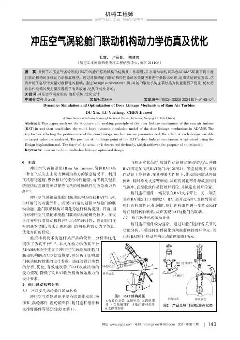
冲压空气涡轮舱门联动机构动力学仿真及优化杜鑫,卢岳良,陈建伟(航空工业南京机电液压工程研究中心,南京211106)摘要:分析了冲压空气涡轮系统(RAT )的舱门联动机构的结构及工作原理,并在运动学仿真平台ADAMS环境下建立舱门联动机构的多体动力学仿真模型。
通过对影响舱门联动机构性能的各关键因素进行参数化处理,运用试验研究方法,仿真分析了各设计变量对目标值的影响。
通过Design exploration工具,对舱门联动机构主要铰接点位置进行了优化,优化后收放作动筒的受力情况得到了有效改善,达到了优化目的。
关键词:冲压空气涡轮系统;连杆机构;优化设计中图分类号:V 228文献标志码:A 文章编号:1002-2333(2021)01-0143-04Dynamics Simulation and Optimization of Door Linkage Mechanism of Ram Air TurbineDU Xin,LU Yueliang,CHEN Jianwei(China Aviation Industry Nanjing Electrical Research Center,Nanjing 211106,China)Abstract:This paper analyzes the structure and working principle of the door linkage mechanism of the ram air turbine (RAT)in and then establishes the multi-body dynamic simulation model of the door linkage mechanism in ADAMS.The key factors affecting the performance of the door linkage mechanism are parameterized,the effect of each design variable on target value are analyzed.The position of the hinge point of the RAT ’s door linkage mechanism is optimized using the Design Exploration tool.The force of the actuator is decreased obviously,which achieves the purpose of optimization.Keywords:ram air turbine;multi-bar linkage;optimized design0引言冲压空气涡轮系统(Ram Air Turbine ,简称RAT )是一种在飞机失去主动力和辅助动力的紧急情况下,利用飞机滑行速度,吸收相对气流的冲压能量,向飞机关键系统提供应急液能源以保持飞机的可操纵性的应急动力系统[1-2]。
组合动力之星:涡轮基组合循环发动机高超声速飞行器可重塑空中战场形态,是21世纪航空航天领域的技术制高点,在军民用领域具有极大的应用前景,目前世界各国在该领域的竞争也是日益激烈。
动力系统是高超声速飞行器的核心,但其对空域、速域、可靠性、环保等要求非常高,导致目前任何一种单一类型的发动机都不能满足上述要求,所以必须发展组合发动机。
目前组合动力方案主要有涡轮-冲压组合动力(TBCC)、火箭-冲压组合动力(RBCC)、涡轮-火箭组合动力(ATR)和三组合发动机(T/RBCC)。
从性能、技术、安全和技术可行性等方面考虑,TBCC 是目前最有希望的高超声速组合动力之一,得到了世界各航空强国的广泛关注和重视。
一、TBCC发动机简介TBCC发动机是将燃气涡轮发动机(涡喷/涡扇)和其它类型发动机(冲压发动机)组合在一起的动力装置,目前已经提出并正在发展的主要有三类:第一类是在高速飞行状态下用冲压发动机提供推力,称为涡轮冲压组合发动机。
按照工作范围划分,可以分为涡轮亚燃冲压发动机和涡轮超燃冲压发动机;按照结构形式划分,可分为串联式和并联式。
第二类是采用进气预冷等先进技术拓宽传统燃气涡轮发动机的工作包线,如超声速强预冷涡轮发动机和膨胀循环空气涡轮冲压发动机等。
第三类是鉴于“推力鸿沟”等TBCC存在的问题,将火箭发动机技术融合进去,如“三喷气”组合循环发动机和空气涡轮冲压发动机等。
典型的TBCC发动机型号主要有:英国反作用发动机公司研制的“佩刀”(SABRE)发动机;美国国防高级研究计划局(DARPA)和美国空军2005年启动的“猎鹰”组合循环发动机项目(FaCET);先进全速域发动机项目(AFRE);膨胀循环空气涡轮冲压发动机。
美国自上世纪50年代便开始了对TBCC发动机的研究工作,目前公认的美国第一款走完设计、研制、生产直至飞行流程的涡轮冲压组合发动机是1956年普惠公司研发的J-58发动机,用于SR-71“黑鸟”高空高速战略侦察机。
专利名称:一种轴对称内并联涡轮基旋转爆震冲压组合发动机及控制方法
专利类型:发明专利
发明人:王卫星,李宥晨,罗龙康,张仁涛
申请号:CN202010629881.9
申请日:20200703
公开号:CN111692013A
公开日:
20200922
专利内容由知识产权出版社提供
摘要:本发明提供了一种轴对称内并联涡轮基旋转爆震冲压组合发动机,采用轴对称布局形式,涡轮发动机位于中间,旋转爆震冲压发动机位于外环流道,进气道唇罩平行移动调节进气道收缩比与流量捕获;通过平行移动模态转换装置,实现发动机三种模态之间转换。
模态转换器前缘处于进气道喉道下游,构建扩张型冲压和涡轮流道,可将结尾激波限制在各自流道内,屏蔽共同工作状态下旋转爆震冲压发动机与涡轮发动机跨流道间的耦合干扰。
唇罩和模态转换装置平行移动的调节方式,具有操作简单、易于实现、可操作性/可靠性强、便于密封等优点。
申请人:南京航空航天大学
地址:210016 江苏省南京市秦淮区御道街29号
国籍:CN
代理机构:南京苏高专利商标事务所(普通合伙)
代理人:张弛
更多信息请下载全文后查看。
涡轮冲压组合发动机燃油系统温升仿真研究
刘友宏;李甲珊;唐世建;陆德雨;董海滨
【期刊名称】《推进技术》
【年(卷),期】2020(41)5
【摘要】为了实现涡轮冲压组合发动机(简称组合发动机)燃油系统温升仿真计算,基于Flowmaster软件平台首次建立了组合发动机燃油系统温升仿真计算模型,为提高精度,根据试验数据自定义了航空煤油随温度压力变化的物性模块代替软件内置物性模块,基于此进行仿真计算得到不同工作模态下燃油系统温升情况。
计算结果表明:涡轮模态工况下自定义物性模块计算得到的主要节点温升与软件内置物性模块相比总体偏低,且压力变化越大计算结果偏差越大;模态转换期间各子燃油系统流量迅速变化对燃油温度影响十分显著;冲压模态工况下燃油流量为2.68倍主燃烧室燃油流量时,可承受的最大发动机热负荷为400kW,最大飞行马赫数为5。
实现了对发动机燃烧室入口燃油温度的预测和评估。
【总页数】8页(P984-991)
【作者】刘友宏;李甲珊;唐世建;陆德雨;董海滨
【作者单位】北京航空航天大学能源与动力工程学院航空发动机气动热力国家级重点实验室;中国航发四川燃气涡轮研究院
【正文语种】中文
【中图分类】V236
【相关文献】
1.航空发动机燃油系统温升特性研究
2.并联式涡轮冲压组合发动机模态转换试验方案研究
3.并联式涡轮冲压组合发动机模态转换试验方案研究
4.涡轮冲压组合发动机涡轮基改型设计研究
5.涡轮基组合循环发动机燃油系统流动传热耦合仿真软件开发
因版权原因,仅展示原文概要,查看原文内容请购买。
涡轮风扇发动机接通加力过程的数值模拟
薛倩;肖洪;廉筱纯
【期刊名称】《航空动力学报》
【年(卷),期】2005(20)4
【摘要】发展了一种低涵道比混合排气加力涡轮风扇发动机接通加力时的数值模拟方法。
该方法考虑混合室加力燃烧室、主燃烧室和外涵道的容积效应,风扇、压气机、高压和低压涡轮等部件的特性,加力燃烧室供油管的充油时间。
以混合室加力燃烧室、主燃烧室和外涵道3个容积室的动态方程为基础,用很小的时间步长逐渐逼近,计算不需要迭代,速度快,精度满足工程要求。
【总页数】4页(P545-548)
【关键词】航空;航天推进系统;涡轮风扇;发动机;接通加力;数值模拟
【作者】薛倩;肖洪;廉筱纯
【作者单位】西北工业大学动力与能源学院
【正文语种】中文
【中图分类】V231
【相关文献】
1.涡轮风扇发动机中过失速性能数值模拟 [J], 郁新华;杨精波;等
2.涡扇发动机加力接通过程延迟控制措施的影响 [J], 郝晓乐;许艳芝;张浩
3.某涡喷发动机接通加力改进方案高空模拟试验研究 [J], 朱青;钟家龙;蒋一鹤
4.涡轮风扇发动机的加力(或排气)混合器类型与特点分析 [J], 陈菊芳
5.涡扇发动机加力接通过程喷管延时调节影响研究 [J], 徐风磊;谢镇波;李边疆;蔡娜;胡强
因版权原因,仅展示原文概要,查看原文内容请购买。