PID控制中英文对照翻译

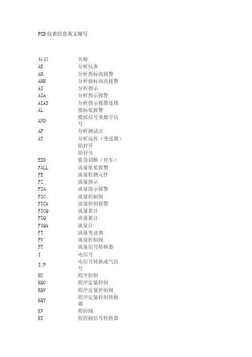
PID仪表信息英文缩写标识名称AE分析仪表AH分析指标高报警AHH分析指标高高报警AI分析指示AIA分析指示报警AIAS分析指示报警连锁AL指标低报警AND 模拟信号变数字信号AP分析测试点AT分析远传（变送器）铅封开铅封关ESD紧急切断（停车）FALL流量低低报警FE流量检测元件FI流量指示FIA流量指示报警FIC流量控制阀FICA流量控制报警FICQ流量累计FIQ流量累计FIQA流量计FT流量变送器FV流量控制阀FY流量信号转换器I电信号I/P 电信号转换成气信号KC程序控制KQC程序定量控制KQV程序定量控制阀KQY 程序定量控制转换器KV程控阀KY程控阀信号转换器LAHS液位高报警连锁LALL液位低低报警LALS液位低LC锁定关报警连锁LG液位计LI液位指示LIA液位指示报警LIAC液位控制报警LIAS液位指示连锁LIC液位控制LICA液位控制报警LICAS液位控制报警连锁LIS液位连锁LIT液位显示信号变送LO锁定开LSH液位高连锁LSL液位低连锁LT液位信号远传LV液位控制阀LY液位信号转换器PAHH压力高高报警PDG数字压力表PDI压差显示PDIA压差显示报警PDICA压差控制报警PDT压差远传PG压力表PI压力显示PIA压力显示报警PIC压力控制信号PICA压力控制报警PICAS压力控制报警连锁PSV压力安全阀PT压力远传PV压力控制阀PY压力信号转换器SHH速度高高报警SIAS速度报警连锁ST速度变速器STOP停止按钮SV安全阀TAHH温度高报警连锁TE温度检测元件TG温度表TI温度指示TIA温度报警TICA温度控制报警TIAS温度报警连锁TIC温度控制阀TICAS温度控制报警连锁TT温度变送器TV气动薄膜控制阀TY电气阀门定位器XV两位控制阀门XY两位控制阀转换器Y信号转换器YL指示灯ZI阀位指示ZIC阀位指示-关ZIO阀位指示-开ZS阀位连锁ZSC阀位开关-关ZSO阀位开关-开ZT阀位变送。

附录Ⅲ 控制理论术语中英文对照表AAbsolute error 绝对误差Accuracy 精确度Active electric network 有源网络Actuating signal 作用信号，启动信号Actuator 执行机构，调节器，激励器Adjust 调整Adaptive control 自适应控制Amplitude 振幅，幅值Analog computer 模拟计算机Analog signal 模拟信号Angle condition 相角条件Angle of arrival 入射角Angle of departure 出射角Angular acceleration 角加速度Argument 辐角Asymptote 渐近线Asymptotically stable 渐近稳定的Automatic control 自动控制Attenuation 衰减Auxiliary equation 辅助方程BBacklash 间隙，回差Bandwidth 带宽Bang-bang control 砰-砰控制，继电控制Biocybernetics 生物控制论Block diagram 方框图，方块图，结构图Bode plot 波特图Breakaway-points 分离点CCAD(computer aided design) 计算机辅助设计Cascade compensation 串联补偿(校正)Cascade control 串级控制Channel 通道Characteristic equation 特征方程Classical control theory 古典控制理论Closed loop control system 闭环控制系统Closed loop frequency response 闭环频率响应Closed loop pole 闭环极点Closed loop zero 闭环零点Combinational control system 复合控制系统Comparator 比较器Comparing element 比较元件，比较环节Compound control 复合控制Compensation 补偿，校正Complex plane 复平面Conditional stability 条件稳定Configuration 结构，配置，方案，组态Constant M loci 等M圆Continuous system 连续系统Controlled variable 被控变量Control system 控制系统Control valve 调节阀Controllability 可控性，能控性Corner frequency 转折频率，交接频率Correcting unit 校正器Correction 校正Coupling 耦合Criterion 判据，准则Critical damping 临界阻尼Cut-off frequency 截止频率Cybernetics 控制论DDamped natural frequency 有阻尼自然频率Damper 阻尼器Damping factor 阻尼系数Damping ratio 阻尼比Dead band 死区Dead time 纯延迟，延迟时间Decomposition 分解Delay 滞后Delay element 滞后环节Derivation action 微分作用Derivative control 微分控制Desired value 预期值，期望值Deviation 偏差Differencing junction 比较点Differential equations 微分方程Digital computer 数字计算机Discrete-data system 离散数据系统Disturbance 扰动，干扰Dominant pole 主导极点Duality 对偶性Dynamic equation 动态方程Dynamic error 动态误差Dynamic process 动态过程EEquilibrium state 平衡状态Eigenvalue 特征值Eigenvector 特征向量Error 误差Error coefficient 误差系数Error signal 误差信号Even symmetry 偶对称Exponential 指数，指数的，幂的Extremum 极值FFeedback 反馈Feedback control 反馈控制Feedback element 反馈环节Feedback path 反馈通道Feedforward 前馈Final value 终值First-order system 一阶系统Forward path 前向通道Frequency 频率Frequency domain 频域Frequency response 频率响应Frequency response characteristic 频率响应特性GGain 增益Gain margin 增益裕度，幅值裕度HHarmonic response 谐波响应Holder 保持器Homogeneous equation 齐次方程Hurwitz determinant 赫尔维茨行列式Hysteresis error 回差IIdealized system 理想化系统Identification 辨识Impulse response 脉冲响应Inertial 惯性的，惯量的，惰性的Inherent characteristic 固有特性Initial condition 初始条件Initial state 初始状态Initial value theorem 初值定理Inner loop 内环Input 输入Input node 输入节点Input signal 输入信号Integral action 积分作用Integral control 积分控制Internal description 内部描述Inverse matrix 逆矩阵Inverse transformation 反变换Inverse Laplace transforms 拉普拉斯反变换Isocline method 等倾线法Iterative algorithm 迭代算法JJordan block 约当块Jordan canonical form 约当标准型KKalman criterion 卡尔曼准则Kalman filter 卡尔曼滤波器LLag network 滞后网络Lag compensation 滞后补偿Laplace transforms 拉普拉斯变换Large scale system 大系统Lead network 超前网络Limit cycle 极限环Linearization 线性化Linearity 线性度Linear equation 线性方程Linear system 线性系统Load-response curve 负荷响应曲线Locus 轨迹Log magnitude 对数幅值Low pass characteristic 低通特性MMagnitude condition 幅值条件Magnitude-Versus-Phase plot 幅值特性曲线Manipulated variable 操纵变量Mason rule 梅森公式Mathematical model 数学模型Matrix 矩阵Maximum overshoot 最大超调量Measurable 可测量的Measured variable 被测变量Minimum phase system 最小相位系统Model decomposition 模型分解Modulus 模Moment of inertia 转动惯量Multinomial 多项式（的）Multivariable system 多变量系统NNatural frequency 自然频率Negative feedback 负反馈Nichols chart 尼柯尔斯图线Node 节点Noise 噪声Nonlinear control system 非线性控制系统Nonminimum phase system 非最小相位系统Nonsingular 非奇异的Norm 范数Numerical control 数字控制Nyquist criterion 奈奎斯特判据Nyquist contour 奈奎斯特轨线OObjective function 目标函数Observability 可观性，能观性Observer 观测器Odd symmetry 奇对称Offset 偏移，位移Open loop 开环Optimal control 最优控制Optimization 最优化Origin 原点Oscillation 振荡Oscillatory response 振荡响应Outer loop 外环Output 输出Output signal 输出信号Over damping 过阻尼Overshoot 超调量PParameter 参数Peak overshoot 超调峰值Peak time 峰值时间Performance index 性能指标Phase lag 相位滞后Phase lead 相位超前Phase margin 相角裕度Phase plane 相平面Pickoff point 引出点PID(proportional plus integral plus derivative) PID(比例、积分、微分)控制器Piece-wise linearization 分段线性化Pole 极点Pole assignment 极点配置Polynomial 多项式Position error 位置误差Positive definiteness 正定性Pre-compensator 预补偿器Process control 过程控制Proportional band 比例带Proportional control 比例控制Pulse 脉冲Pulse width 脉宽Pure delay 纯滞后RRamp input 斜坡输入Ramp response 斜坡响应Rate feedback 速度反馈Rate time 微分时间，预调时间Rational 有理(数)的，合理的Realization 实现Reference variable 参考变量Regulator 调节器Relative stability 相对稳定Reliability 可靠性Response 响应Reset time 再调时间，积分时间Residue 留数Rise time 上升时间Roots loci 根轨迹Routh-Hurwitz criterion 劳斯-赫尔维茨判据Routh stability criterion 劳斯稳定判据SSampling control 采样控制Sampling freqency 采样频率Sampling period 采样周期Series compensation 串联补偿Servo 伺服机构，伺服电机Servodrive 伺服传动，伺服转动装置Set value 设定值Settling time 调节时间，稳定时间Signal flow graph 信号流图Singular point 奇点Stability 稳定（性）Stability margin 稳定裕度State equations 状态方程State space 状态空间State variables 状态变量Steady-state 稳态的Stationary 稳态Steady-state deviation 稳态偏差Steady-state error 稳态误差Step singal 阶跃信号Step response 阶跃响应Stochastic process 随机过程Summing junction 相加点Superposition 叠加Systematic deviation 系统偏差System identification 系统辨识TTangent 切线Threshold value 阈值Time constant 时间常数Time domain 时域Time response 时间响应Time-invariant system 常定(时不变)系统Time-varying system 时变系统Trajectory 轨迹Transducer 传感器，变换器Transfer function 传递函数Transfer matrix 转移矩阵Transient response 暂态响应Transmitter 变送器Transportation lag 传输滞后UUndamped natural frequency 无阻尼自然频率Underdamping 欠阻尼Uniform stability 一致稳定Unit circle 单位圆Unit impulse 单位脉冲Unit step function 单位阶跃函数Unity feedback 单位反馈Unity matrix 单位矩阵Unstable 不稳定的Asymmetrical 不对称的VValue of quantity 量值variable 变量Vector 向量Velocity feedback 速度反馈WWaveform 波形Weighting function 加权函数White noise 白噪声ZZero 零点Zero input response 零点输入响应Zero-order holder 零阶保持器Zero-state response 零状态响应Z-transfer function Z传递函数Z-transformation Z变换。

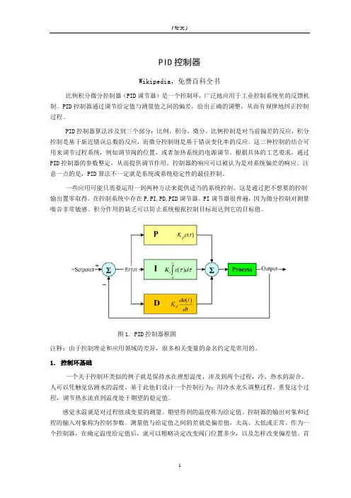
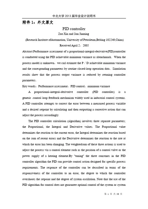
PID控制器Wikipedia，免费百科全书比例积分微分控制器（PID调节器）是一个控制环，广泛地应用于工业控制系统里的反馈机制。

PID控制器通过调节给定值与测量值之间的偏差，给出正确的调整，从而有规律地纠正控制过程。

PID控制器算法涉及到三个部分：比例，积分，微分。

比例控制是对当前偏差的反应，积分控制是基于新近错误总数的反应，而微分控制则是基于错误变化率的反应。

这三种控制的结合可用来调节过程系统，例如调节阀的位置，或者加热系统的电源调节。

根据具体的工艺要求，通过PID控制器的参数整定，从而提供调节作用。

控制器的响应可以被认为是对系统偏差的响应。

注意一点的是，PID算法不一定就是系统或系统稳定性的最佳控制。

一些应用可能只需要运用一到两种方法来提供适当的系统控制。

这是通过把不想要的控制输出置零取得。

在控制系统中存在P,PI,PD,PID调节器。

PI调节器很普遍，因为微分控制对测量噪音非常敏感。

积分作用的缺乏可以防止系统根据控制目标而达到它的目标值。

图1. PID控制器框图注释：由于控制理论和应用领域的差异，很多相关变量的命名约定是常用的。

1．控制环基础一个关于控制环类似的例子就是保持水在理想温度，涉及到两个过程，冷、热水的混合。

人可以凭触觉估测水的温度。

基于此他们设计一个控制行为：用冷水龙头调整过程。

重复这个过程，调节热水流直到温度处于期望的稳定值。

感觉水温就是对过程值或变量的测量。

期望得到的温度称为给定值。

控制器的输出对象和过程的输入对象称为控制参数。

测量值与给定值之间的差就是偏差值，太高、太低或正常。

作为一个控制器，在确定温度给定值后，就可以粗略决定改变阀门位置多少，以及怎样改变偏差值。

首次估计即是PID 控制器的比例度的确定。

当它几乎正确时，PID控制器的积分作用就是起着逐渐调整温度的作用。

微分作用就是根据水温变得更热、更冷，以及变化速率来决定什么时候、怎样调整那些阀门。

当偏差小时而做了一个大变动，相当于一个大的调整控制器，会导致超调。

附件1：外文原文PID controllerZuo Xin and Sun Jinming(Research Institute ofAutomation, University of Petroleum,Belting 102249,China)Received April 2，2005Abstract:Performance assessment of a proportional-integral-derivative(PID)controller is condueted using the PID achievable minimum variance as abenchmark．When the process model is unknown，we carl estimate the P／D·achievable minimum variance and the corresponding parameters by routine closed-loop operation data．Simulation results show that the process output variance is reduced by retuning controller parameters．Key words：Performance assessment，PID control，minimum varianceA proportional–integral–derivative controller (PID controller) is a generic .control loop feedback mechanism widely used in industrial control systems.A PID controller attempts to correct the error between a measured process variable and a desired setpoint by calculating and then outputting a corrective action that can adjust the process accordingly.The PID controller calculation (algorithm) involves three separate parameters; the Proportional, the Integral and Derivative values. The Proportional value determines the reaction to the current error, the Integral determines the reaction based on the sum of recent errors and the Derivative determines the reaction to the rate at which the error has been changing. The weightedsum of these three actions is used to adjust the process via a control element such as the position of a control valve or the power supply of a heating element.By "tuning" the three constants in the PID controller algorithm the PID can provide control action designed for specific process requirements. The response of the controller can be described in terms of the responsiveness of the controller to an error, the degree to which the controller overshoots the setpoint and the degree of system oscillation. Note that the use of the PID algorithm for control does not guarantee optimal control of the system or systemstability.Some applications may require using only one or two modes to provide the appropriate system control. This is achieved by setting the gain of undesired control outputs to zero. A PID controller will be called a PI, PD, P or I controller in the absence of the respective control actions. PI controllers are particularly common, since derivative action is very sensitive to measurement noise, and the absence of an integral value may prevent the system from reaching its target value due to the control action.Note: Due to the diversity of the field of control theory and application, many naming conventions for the relevant variables are in common use.1.Control loop basicsA familiar example of a control loop is the action taken to keep one's shower water at the ideal temperature, which typically involves the mixing of two process streams, cold and hot water. The person feels the water to estimate its temperature. Based on this measurement they perform a control action: use the cold water tap to adjust the process. The person would repeat this input-output control loop, adjusting the hot water flow until the process temperature stabilized at the desired value.Feeling the water temperature is taking a measurement of the process value or process variable (PV). The desired temperature is called the setpoint (SP). The output from the controller and input to the process (the tap position) is called the manipulated variable (MV). The difference between the measurement and the setpoint is the error (e), too hot or too cold and by how much.As a controller, one decides roughly how much to change the tap position (MV) after one determines the temperature (PV), and therefore the error. This first estimate is the equivalent of the proportional action of a PID controller. The integral action of a PID controller can be thought of as gradually adjusting the temperature when it is almost right. Derivative action can be thought of as noticing the water temperature is getting hotter or colder, and how fast, and taking that into account when deciding how to adjust the tap.Making a change that is too large when the error is small is equivalent to a high gain controller and will lead toovershoot. If the controller were to repeatedly make changes that were too large and repeatedly overshoot the target, this control loop would be termed unstable and the output would oscillate around the setpoint in either a constant, growing, or decaying sinusoid. A human would not do this because we are adaptive controllers, learning from the process history, but PID controllers do not have the ability to learn and must be set up correctly. Selecting the correct gains for effective control is known as tuning the controller.If a controller starts from a stable state at zero error (PV = SP), then further changes by the controller will be in response to changes in other measured or unmeasured inputs to the process that impact on the process, and hence on the PV. Variables that impact on the process other than the MV are known as disturbances and generally controllers are used to reject disturbances and/or implement setpoint changes. Changes in feed water temperature constitute a disturbance to the shower process.In theory, a controller can be used to control any process which has a measurable output (PV), a known ideal value for that output (SP) and an input to the process (MV) that will affect the relevant PV. Controllers are used in industry to regulate temperature, pressure, flow rate, chemical composition, speed and practically every other variable for which a measurement exists. Automobile cruise control is an example of a process which utilizes automated control.Due to their long history, simplicity, well grounded theory and simple setup and maintenance requirements, PID controllers are the controllers of choice for many of these applications.2.PID controller theoryNote: This section describes the ideal parallel or non-interacting form of the PID controller. For other forms please see the Section "Alternative notation and PID forms".The PID control scheme is named after its three correcting terms, whose sum constitutes the manipulated variable (MV). Hence:Where Pout, Iout, and Dout are the contributions to the output from the PID controller from each of the three terms, as defined below.2.1. Proportional termThe proportional term makes a change to the output that is proportional to the current error value. The proportional response can be adjusted by multiplying the error by a constant Kp, called the proportional gain.The proportional term is given by:WherePout: Proportional outputKp: Proportional Gain, a tuning parametere: Error = SP − PVt: Time or instantaneous time (the present)Change of response for varying KpA high proportional gain results in a large change in the output for a given change in the error. If the proportional gain is too high, the system can become unstable (See the section on Loop Tuning). In contrast, a small gain results in a small output response to a large input error, and a less responsive (or sensitive) controller. If the proportional gain is too low, the control action may be too small when responding to system disturbances.In the absence of disturbances, pure proportional control will not settle at its target value, but will retain a steady state error that is a function of the proportional gain and the process gain. Despite the steady-state offset, both tuning theory and industrial practice indicate that it is the proportional term that should contribute the bulk of the output change.2.2.Integral termThe contribution from the integral term is proportional to both the magnitude of the error and the duration of the error. Summing the instantaneous error over time (integrating the error) gives the accumulated offset that should have been correctedpreviously. The accumulated error is then multiplied by the integral gain and added to the controller output. The magnitude of the contribution of the integral term to the overall control action is determined by the integral gain, Ki.The integral term is given by:Iout: Integral outputKi: Integral Gain, a tuning parametere: Error = SP − PVτ: Time in the past contributing to the integral responseThe integral term (when added to the proportional term) accelerates the movement of the process towards setpoint and eliminates the residual steady-state error that occurs with a proportional only controller. However, since the integral term is responding to accumulated errors from the past, it can cause the present value to overshoot the setpoint value (cross over the setpoint and then create a deviation in the other direction). For further notes regarding integral gain tuning and controller stability, see the section on loop tuning.2.3 Derivative termThe rate of change of the process error is calculated by determining the slope of the error over time (i.e. its first derivative with respect to time) and multiplying this rate of change by the derivative gain Kd. The magnitude of the contribution of the derivative term to the overall control action is termed the derivative gain, Kd.The derivative term is given by:Dout: Derivative outputKd: Derivative Gain, a tuning parametere: Error = SP − PVt: Time or instantaneous time (the present)The derivative term slows the rate of change of the controller output and this effect is most noticeable close to the controller setpoint. Hence, derivative control is used to reduce the magnitude of the overshoot produced by the integral component and improve the combined controller-process stability. However, differentiation of a signal amplifies noise and thus this term in the controller is highly sensitive to noise in the error term, and can cause a process to become unstable if the noise and the derivative gain are sufficiently large.2.4 SummaryThe output from the three terms, the proportional, the integral and the derivative terms are summed to calculate the output of the PID controller. Defining u(t) as the controller output, the final form of the PID algorithm is:and the tuning parameters areKp: Proportional Gain - Larger Kp typically means faster response since thelarger the error, the larger the Proportional term compensation. An excessively large proportional gain will lead to process instability and oscillation.Ki: Integral Gain - Larger Ki implies steady state errors are eliminated quicker. The trade-off is larger overshoot: any negative error integrated during transient response must be integrated away by positive error before we reach steady state.Kd: Derivative Gain - Larger Kd decreases overshoot, but slows down transient response and may lead to instability due to signal noise amplification in the differentiation of the error.3. Loop tuningIf the PID controller parameters (the gains of the proportional, integral and derivative terms) are chosen incorrectly, the controlled process input can be unstable, i.e. its output diverges, with or without oscillation, and is limited only by saturation or mechanical breakage. Tuning a control loop is the adjustment of its control parameters (gain/proportional band, integral gain/reset, derivative gain/rate) to the optimumvalues for the desired control response.The optimum behavior on a process change or setpoint change varies depending on the application. Some processes must not allow an overshoot of the process variable beyond the setpoint if, for example, this would be unsafe. Other processes must minimize the energy expended in reaching a new setpoint. Generally, stability of response (the reverse of instability) is required and the process must not oscillate for any combination of process conditions and setpoints. Some processes have a degree of non-linearity and so parameters that work well at full-load conditions don't work when the process is starting up from no-load. This section describes some traditional manual methods for loop tuning.There are several methods for tuning a PID loop. The most effective methods generally involve the development of some form of process model, then choosing P, I, and D based on the dynamic model parameters. Manual tuning methods can be relatively inefficient.The choice of method will depend largely on whether or not the loop can be taken "offline" for tuning, and the response time of the system. If the system can be taken offline, the best tuning method often involves subjecting the system to a step change in input, measuring the output as a function of time, and using this response to determine the control parameters.Choosing a Tuning MethodMethodAdvantagesDisadvantagesManual TuningNo math required. Online method.Requires experiencedpersonnel.Ziegler–NicholsProven Method. Online method.Process upset, sometrial-and-error, very aggressive tuning.Software ToolsConsistent tuning. Online or offline method. May includevalve and sensor analysis. Allow simulation before downloading.Some cost and training involved.Cohen-CoonGood process models.Some math. Offline method. Onlygood for first-order processes.3.1 Manual tuningIf the system must remain online, one tuning method is to first set the I and D values to zero. Increase the P until the output of the loop oscillates, then the P should be left set to be approximately half of that value for a "quarter amplitude decay" type response. Then increase D until any offset is correct in sufficient time for the process. However, too much D will cause instability. Finally, increase I, if required, until the loop is acceptably quick to reach its reference after a load disturbance. However, too much I will cause excessive response and overshoot. A fast PID loop tuning usually overshoots slightly to reach the setpoint more quickly; however, some systems cannot accept overshoot, in which case an "over-damped" closed-loop system is required, which will require a P setting significantly less than half that of the P setting causing oscillation.3.2Ziegler–Nichols methodAnother tuning method is formally known as the Ziegler–Nichols method, introduced by John G. Ziegler and Nathaniel B. Nichols. As in the method above, the I and D gains are first set to zero. The "P" gain is increased until it reaches the "critical gain" Kc at which the output of the loop starts to oscillate. Kc and the oscillation period Pc are used to set the gains as shown:3.3 PID tuning softwareMost modern industrial facilities no longer tune loops using the manual calculation methods shown above. Instead, PID tuning and loop optimization software are used to ensure consistent results. These software packages will gather the data, develop process models, and suggest optimal tuning. Some software packages can even develop tuning by gathering data from reference changes.Mathematical PID loop tuning induces an impulse in the system, and then uses the controlled system's frequency response to design the PID loop values. In loops with response times of several minutes, mathematical loop tuning is recommended, because trial and error can literally take days just to find a stable set of loop values.Optimal values are harder to find. Some digital loop controllers offer a self-tuning feature in which very small setpoint changes are sent to the process, allowing the controller itself to calculate optimal tuning values.Other formulas are available to tune the loop according to different performance criteria.4 Modifications to the PID algorithmThe basic PID algorithm presents some challenges in control applications that have been addressed by minor modifications to the PID form.One common problem resulting from the ideal PID implementations is integralwindup. This can be addressed by:Initializing the controller integral to a desired valueDisabling the integral function until the PV has entered the controllable region Limiting the time period over which the integral error is calculatedPreventing the integral term from accumulating above or below pre-determined boundsMany PID loops control a mechanical device (for example, a valve). Mechanical maintenance can be a major cost and wear leads to control degradation in the form of either stiction or a deadband in the mechanical response to an input signal. The rate of mechanical wear is mainly a function of how often a device is activated to make a change. Where wear is a significant concern, the PID loop may have an output deadband to reduce the frequency of activation of the output (valve). This is accomplished by modifying the controller to hold its output steady if the change would be small (within the defined deadband range). The calculated output must leave the deadband before the actual output will change.The proportional and derivative terms can produce excessive movement in the output when a system is subjected to an instantaneous "step" increase in the error, such as a large setpoint change. In the case of the derivative term, this is due to taking the derivative of the error, which is very large in the case of an instantaneous step change.5. Limitations of PID controlWhile PID controllers are applicable to many control problems, they can perform poorly in some applications.PID controllers, when used alone, can give poor performance when the PID loop gains must be reduced so that the control system does not overshoot, oscillate or "hunt" about the control setpoint value. The control system performance can be improved by combining the feedback (or closed-loop) control of a PID controller with feed-forward (or open-loop) control. Knowledge about the system (such as the desired acceleration and inertia) can be "fed forward" and combined with the PID output to improve the overall system performance. The feed-forward value alone can often provide the major portion of the controller output. The PID controller can then be used primarily to respond to whatever difference or "error" remains between the setpoint (SP) and the actual value of the process variable (PV). Since the feed-forward output is not affected by the process feedback, it can never cause the control system to oscillate, thus improving the system response and stability.For example, in most motion control systems, in order to accelerate a mechanical load under control, more force or torque is required from the prime mover, motor, or actuator. If a velocity loop PID controller is being used to control the speed of the load and command the force or torque being applied by the prime mover, then it is beneficial to take the instantaneous acceleration desired for the load, scale that value appropriately and add it to the output of the PID velocity loop controller. This means that whenever the load is being accelerated or decelerated, a proportional amount of force is commanded from the prime mover regardless of the feedback value. The PID loop in this situation uses the feedback information to effect any increase or decrease of the combined output in order to reduce the remaining difference between the process setpoint and thefeedback value. Working together, the combined open-loop feed-forward controller and closed-loop PID controller can provide a more responsive, stable and reliable control system.Another problem faced with PID controllers is that they are linear. Thus, performance of PID controllers in non-linear systems (such as HV AC systems) isvariable. Often PID controllers are enhanced through methods such as PID gain scheduling or fuzzy logic. Further practical application issues can arise from instrumentation connected to the controller. A high enough sampling rate, measurement precision, and measurement accuracy are required to achieve adequate control performance.A problem with the Derivative term is that small amounts of measurement or process noise can cause large amounts of change in the output. It is often helpful to filter the measurements with a low-pass filter in order to remove higher-frequency noise components. However, low-pass filtering and derivative control can cancel each other out, so reducing noise by instrumentation means is a much better choice. Alternatively, the differential band can be turned off in many systems with little loss of control. This is equivalent to using the PID controller as a PI controller.6. Cascade controlOne distinctive advantage of PID controllers is that two PID controllers can be used together to yield better dynamic performance. This is called cascaded PID control. In cascade control there are two PIDs arranged with one PID controlling the set point of another. A PID controller acts as outer loop controller, which controls the primary physical parameter, such as fluid level or velocity. The other controller acts as inner loop controller, which reads the output of outer loop controller as set point, usually controlling a more rapid changing parameter, flowrate or accelleration. It can be mathematically proved that the working frequency of the controller is increased and the time constant of the object is reduced by using cascaded PID controller.[vague]7. Physical implementation of PID controlIn the early history of automatic process control the PID controller was implemented as a mechanical device. These mechanical controllers used a lever, spring and a mass and were often energized by compressed air. These pneumatic controllers were once the industry standard.Electronic analog controllers can be made from a solid-state or tube amplifier, a capacitor and a resistance. Electronic analogPID control loops were often found within more complex electronic systems, for example, the head positioning of a disk drive, the power conditioning of a power supply, or even the movement-detection circuit of a modern seismometer. Nowadays, electronic controllers have largely been replaced by digital controllers implemented with microcontrollers or FPGAs.Most modern PID controllers in industry are implemented in software in programmable logic controllers (PLCs) or as a panel-mounted digital controller. Software implementations have the advantages that they are relatively cheap and are flexible with respect to the implementation of the PID algorithm.References[1]Byung，S.K.(2000)On Performance Assessment of Feedback Control Loops．Austin：The University of Texas Austin[2]Desborough，L．and Harris，T.(1992)Performance Assessment Measures for Univariate Feedback Control. The Canadian Journal of Chemical Engineering,70(12)．1186-1197[3]Ender,D.B.(1993)Process Control Performance：Not as Good as You Think．Control Engineering，40(10)[4]Harris,T(1993)Pefformance Assessment Measllres for Univariate Feedforward/Feedback Control．The Canadian Journal of Chemical Engineering，71(8)，1186-1197[5]Qin，S．J．(1 998)Contr01 Performance Monitoring： A Review and Assessment．Com．Chem．Eng．，(23)，173．186[6]Sun,Jinming(2004)PID Performance Assessment and Parameters Tuning．Beijing：China University of Petroleum[7]Xu，Xi；Li，Tao and Bo，Xiaochen(2000)Matlab Toolbox Application--Control Engineering．Bering：Electron Industry Press附件2：外文资料翻译译文PID控制器左信孙金明（石油大学自动化研究所，北京，102249，中国）发表于2005.4.2摘要：一个比例积分微分（PID）控制器的性能评价进行使用PID实现的最小方差作为参照。

pid的专业表达PID，全称比例-积分-微分控制器（Proportional-Integral-Derivative Controller），是一种广泛用于控制系统的反馈控制器。

在自动化、过程控制、航空航天、机器人等领域，PID控制器被用于调节各种物理量，如温度、压力、流量、速度等，以达到预定的目标值。

PID控制器基于比例、积分和微分三个基本控制作用进行工作。

这三个控制作用分别对应于误差的不同方面，通过组合这三个作用，PID控制器能够有效地减小系统误差并提高控制精度。

比例控制（P控制）是PID控制的基础，它根据当前误差的大小来调整控制输出。

如果误差较大，则增大输出；如果误差较小，则减小输出。

通过调整比例系数，可以改变系统对误差的敏感度，从而影响系统的调节速度和稳定性。

积分控制（I控制）主要用于消除静差，提高系统的无差度。

积分项会对误差进行积分，随着时间的推移，即使误差很小，积分项也会逐渐增大。

因此，积分作用可以消除长期存在的误差。

通过调整积分系数，可以平衡系统的调节速度和静差消除能力。

微分控制（D控制）能够预测误差的变化趋势，从而提前增大或减小控制输出，改善系统的动态特性。

微分项会对误差的变化率进行控制，当误差增大时，微分项会提前增大输出；当误差减小时，微分项会提前减小输出。

这有助于减小超调和缩短调节时间。

在实际应用中，PID控制器通常需要根据特定的控制系统进行调整和优化。

这包括选择合适的比例系数、积分系数和微分系数，以及考虑其他因素如控制对象的特性和扰动的变化等。

为了实现最佳的控制效果，可能需要反复试验和调整PID参数。

除了基本的PID控制器，还有许多改进的PID控制器变体，如PI控制器、PD控制器、PID-FF控制器等。

这些变体在某些特定情况下可能更适合特定的控制需求。

总的来说，PID控制器是一种强大而灵活的控制工具，其专业表达涵盖了比例、积分和微分三个基本组成部分以及它们在控制系统中的重要性和作用。

自动化控制英文缩写解释自动化控制（Automation Control）是指利用各种自动化技术和设备，对生产过程、工业设备、机械系统、电力系统等进行监测、控制和调节的过程。

为了方便交流和表达，自动化控制领域中常使用一些英文缩写来表示特定的概念和术语。

下面是一些常见的自动化控制英文缩写及其解释：1. PLC：Programmable Logic Controller，可编程逻辑控制器。

PLC是一种专门用于工业自动化控制的计算机控制系统，它能够监测输入信号、进行逻辑运算并输出控制信号，实现对工业过程的自动化控制。

2. DCS：Distributed Control System，分散控制系统。

DCS是一种分布式的控制系统，通过将控制功能分散在多个控制器中，实现对整个工业过程的集中控制和管理。

3. SCADA：Supervisory Control And Data Acquisition，监控与数据采集系统。

SCADA系统用于监测和控制远程设备和过程，通过采集实时数据、进行数据处理和分析，实现对工业过程的监控和管理。

4. HMI：Human Machine Interface，人机界面。

HMI是人与机器之间进行信息交互的界面，通常采用触摸屏、键盘、指示灯等设备，用于操作和监视自动化控制系统。

5. PID：Proportional-Integral-Derivative，比例-积分-微分控制。

PID控制是一种常用的自动控制算法，通过比例、积分和微分三个部份的组合，实现对控制系统的稳定性和响应速度的调节。

6. CNC：Computer Numerical Control，数控。

CNC是一种通过计算机控制数值信号，实现对机床、机器人等设备进行精确控制的技术。

7. MES：Manufacturing Execution System，创造执行系统。

MES系统用于管理和控制创造过程中的各个环节，包括计划排程、生产监控、质量管理等，实现对创造过程的优化和管理。

PID controllerA proportional–integral–derivative controller (PID controller) is a generic .control loop feedback mechanism widely used in industrial control systems. A PID controller attempts to correct the error between a measured process variable and a desired setpoint by calculating and then outputting a corrective action that can adjust the process accordingly.The PID controller calculation (algorithm) involves three separate parameters; the Proportional, the Integral and Derivative values. The Proportional value determines the reaction to the current error, the Integral determines the reaction based on the sum of recent errors and the Derivative determines the reaction to the rate at which the error has been changing. The weightedsum of these three actions is used to adjust the process via a control element such as the position of a control valve or the power supply of a heating element.By "tuning" the three constants in the PID controller algorithm the PID can provide control action designed for specific process requirements. The response of the controller can be described in terms of the responsiveness of the controller to an error, the degree to which the controller overshoots the setpoint and the degree of system oscillation. Note that the use of the PID algorithm for control does not guarantee optimal control of the system or system stability.Some applications may require using only one or two modes to provide the appropriate system control. This is achieved by setting the gain of undesired control outputs to zero. A PID controller will be called a PI, PD, P or I controller in the absence of the respective control actions. PI controllers are particularly common, since derivative action is very sensitive to measurement noise, and the absence of an integral value may prevent the system from reaching its target value due to the control action.Note: Due to the diversity of the field of control theory and application, many naming conventions for the relevant variables are in common use.1.Control loop basicsA familiar example of a control loop is the action taken to keep one's shower water at the ideal temperature, which typically involves the mixing of two process streams, cold and hot water. The person feels the water to estimate its temperature. Based on this measurement they perform a control action: use the cold water tap to adjust the process. The person would repeat this input-output control loop, adjusting the hot water flow until the process temperature stabilized at the desired value.Feeling the water temperature is taking a measurement of the process value or process variable (PV). The desired temperature is called the setpoint (SP). The output from the controller and input to the process (the tap position) is called the manipulated variable (MV). The difference between the measurement and the setpoint is the error (e), too hot or too cold and by how much.As a controller, one decides roughly how much to change the tap position (MV) after one determines the temperature (PV), and therefore the error. This first estimate is the equivalent of the proportional action of a PID controller. The integral action of a PID controller can be thought of as gradually adjusting the temperature when it is almost right. Derivative action can be thought of as noticing the water temperature is getting hotter or colder, and how fast, and taking that into account when deciding how to adjust the tap.Making a change that is too large when the error is small is equivalent to a high gain controller and will lead to overshoot. If the controller were to repeatedly make changes that were too large and repeatedly overshoot the target, this control loop would be termed unstable and the output would oscillate around the setpoint in either a constant, growing, or decaying sinusoid. A human would not do this because we are adaptive controllers, learning from the process history, but PID controllers do not have the ability to learn and must be set up correctly. Selectingthe correct gains for effective control is known as tuning the controller.If a controller starts from a stable state at zero error (PV = SP), then further changes by the controller will be in response to changes in other measured or unmeasured inputs to the process that impact on the process, and hence on the PV. Variables that impact on the process other than the MV are known as disturbances and generally controllers are used to reject disturbances and/or implement setpoint changes. Changes in feed water temperature constitute a disturbance to the shower process.In theory, a controller can be used to control any process which has a measurable output (PV), a known ideal value for that output (SP) and an input to the process (MV) that will affect the relevant PV. Controllers are used in industry to regulate temperature, pressure, flow rate, chemical composition, speed and practically every other variable for which a measurement exists. Automobile cruise control is an example of a process which utilizes automated control.Due to their long history, simplicity, well grounded theory and simple setup and maintenance requirements, PID controllers are the controllers of choice for many of these applications.2.PID controller theoryNote: This section describes the ideal parallel or non-interacting form of the PID controller. For other forms please see the Section "Alternative notation and PID forms".The PID control scheme is named after its three correcting terms, whose sum constitutes the manipulated variable (MV). Hence:where Pout, Iout, and Dout are the contributions to the output from the PID controller from each of the three terms, as defined below.2.1. Proportional termThe proportional term makes a change to the output that is proportional to the current error value. The proportional response can be adjusted by multiplying the error by a constant Kp, called the proportional gain.The proportional term is given by:WherePout: Proportional outputKp: Proportional Gain, a tuning parametere: Error = SP − PVt: Time or instantaneous time (the present)Change of response for varying KpA high proportional gain results in a large change in the output for a given change in the error. If the proportional gain is too high, the system can become unstable (See the section on Loop Tuning). In contrast, a small gain results in a small output response to a large input error, and a less responsive (or sensitive) controller. If the proportional gain is too low, the control action may be too small when responding to system disturbances.In the absence of disturbances, pure proportional control will not settle at its target value, but will retain a steady state error that is a function of the proportional gain and the process gain. Despite the steady-state offset, both tuning theory and industrial practice indicate that it is the proportional term that should contribute the bulk of the output change.2.2.Integral termThe contribution from the integral term is proportional to both the magnitude of the error and the duration of the error. Summing the instantaneous error over time (integrating the error) gives the accumulated offset that should have been corrected previously. The accumulated error is then multiplied by the integral gain and added to the controller output. The magnitude of the contribution of the integral term to the overall control action is determined by the integral gain, Ki.The integral term is given by:Iout: Integral outputKi: Integral Gain, a tuning parametere: Error = SP − PVτ: Time in the past contributing to the integral responseThe integral term (when added to the proportional term) accelerates the movement of the process towards setpoint and eliminates the residual steady-state error that occurs with a proportional only controller. However, since the integral term is responding to accumulated errors from the past, it can cause the present value to overshoot the setpoint value (cross over the setpoint and then create a deviation in the other direction). For further notes regarding integral gain tuning and controller stability, see the section on loop tuning.2.3 Derivative termThe rate of change of the process error is calculated by determining the slope of the error over time (i.e. its first derivative with respect to time) and multiplying this rate of change by the derivative gain Kd. The magnitude of the contribution of the derivative term to the overall control action is termed the derivative gain, Kd.The derivative term is given by:Dout: Derivative outputKd: Derivative Gain, a tuning parametere: Error = SP − PVt: Time or instantaneous time (the present)The derivative term slows the rate of change of the controller output and this effect is most noticeable close to the controller setpoint. Hence, derivative control is used to reduce the magnitude of the overshoot produced by the integral component and improve the combined controller-process stability. However, differentiation of a signal amplifies noise and thus this term in the controller is highly sensitive to noise in the error term, and can cause a process to become unstable if the noise and the derivative gain are sufficiently large.2.4 SummaryThe output from the three terms, the proportional, the integral and the derivative terms are summed to calculate the output of the PID controller. Defining u(t) as the controller output, the final form of the PID algorithm is:and the tuning parameters areKp: Proportional Gain - Larger Kp typically means faster response since thelarger the error, the larger the Proportional term compensation. An excessively large proportional gain will lead to process instability and oscillation.Ki: Integral Gain - Larger Ki implies steady state errors are eliminated quicker. The trade-off is larger overshoot: any negative error integrated during transient response must be integrated away by positive error before we reach steady state.Kd: Derivative Gain - Larger Kd decreases overshoot, but slows down transient response and may lead to instability due to signal noise amplification in the differentiation of the error.3. Loop tuningIf the PID controller parameters (the gains of the proportional, integral and derivative terms) are chosen incorrectly, the controlled process input can be unstable, i.e. its output diverges, with or without oscillation, and is limited only by saturation or mechanical breakage. Tuning a control loop is the adjustment of its control parameters (gain/proportional band, integral gain/reset, derivative gain/rate) to the optimum values for the desired control response.The optimum behavior on a process change or setpoint change varies depending on the application. Some processes must not allow an overshoot of the process variable beyond the setpoint if, for example, this would be unsafe. Other processes must minimize the energy expended in reaching a new setpoint. Generally, stability of response (the reverse of instability) is required and the process must not oscillate for any combination of process conditions and setpoints. Some processes have a degree of non-linearity and so parameters that work well at full-load conditions don't work when the process is starting up from no-load. This section describes some traditional manual methods for loop tuning.There are several methods for tuning a PID loop. The most effective methods generally involve the development of some form of process model, then choosing P, I, and D based on the dynamic model parameters. Manual tuning methods can be relatively inefficient.The choice of method will depend largely on whether or not the loop can be taken "offline" for tuning, and the response time of the system. If the system can be taken offline, the best tuning method often involves subjecting the system to a step change in input, measuring the output as a function of time, and using this response to determine the control parameters.Choosing a Tuning MethodMethodAdvantagesDisadvantagesManual TuningNo math required. Online method.Requires experiencedpersonnel.Ziegler–NicholsProven Method. Online method.Process upset, sometrial-and-error, very aggressive tuning.Software ToolsConsistent tuning. Online or offline method. May includevalve and sensor analysis. Allow simulation before downloading.Some costand training involved.Cohen-CoonGood process models.Some math. Offline method. Only good forfirst-order processes.3.1 Manual tuningIf the system must remain online, one tuning method is to first set the I and D values to zero. Increase the P until the output of the loop oscillates, then the P should be left set to be approximately half of that value for a "quarter amplitude decay" type response. Then increase D until any offset is correct in sufficienttime for the process. However, too much D will cause instability. Finally, increase I, if required, until the loop is acceptably quick to reach its reference after a load disturbance. However, too much I will cause excessive response and overshoot. A fast PID loop tuning usually overshoots slightly to reach the setpoint more quickly; however, some systems cannot accept overshoot, in which case an "over-damped" closed-loop system is required, which will require a P setting significantly less than half that of the P setting causing oscillation.3.2Ziegler–Nichols methodAnother tuning method is formally known as the Ziegler–Nichols method, introduced by John G. Ziegler and Nathaniel B. Nichols. As in the method above, the I and D gains are first set to zero. The "P" gain is increased until it reaches the "critical gain" Kc at which the output of the loop starts to oscillate. Kc and the oscillation period Pc are used to set the gains as shown:3.3 PID tuning softwareMost modern industrial facilities no longer tune loops using the manual calculation methods shown above. Instead, PID tuning and loop optimization software are used to ensure consistent results. These software packages will gather the data, develop process models, and suggest optimal tuning. Some software packages can even develop tuning by gathering data from reference changes.Mathematical PID loop tuning induces an impulse in the system, and then uses the controlled system's frequency response to design the PID loop values. In loops with response times of several minutes, mathematical loop tuning is recommended, because trial and error can literally take days just to find a stable set of loop values. Optimal values are harder to find. Some digital loop controllers offer a self-tuning feature in which very small setpoint changes are sent to the process, allowing the controller itself to calculate optimal tuning values.Other formulas are available to tune the loop according to different performance criteria.4 Modifications to the PID algorithmThe basic PID algorithm presents some challenges in control applications that have been addressed by minor modifications to the PID form.One common problem resulting from the ideal PID implementations is integralwindup. This can be addressed by:Initializing the controller integral to a desired valueDisabling the integral function until the PV has entered the controllable regionLimiting the time period over which the integral error is calculatedPreventing the integral term from accumulating above or below pre-determined boundsMany PID loops control a mechanical device (for example, a valve). Mechanical maintenance can be a major cost and wear leads to control degradation in the form of either stiction or a deadband in the mechanical response to an input signal. The rate of mechanical wear is mainly a function of how often a device is activated to make a change. Where wear is a significant concern, the PID loop may have an output deadband to reduce the frequency of activation of the output (valve). This is accomplished by modifying the controller to hold its output steady if the change would be small (within the defined deadband range). The calculated output must leave the deadband before the actual output will change.The proportional and derivative terms can produce excessive movement in the output when a system is subjected to an instantaneous "step" increase in the error, such as a large setpoint change. In the case of the derivative term, this is due to taking the derivative of the error, which is very large in the case of an instantaneous step change.5. Limitations of PID controlWhile PID controllers are applicable to many control problems, they can perform poorly in some applications.PID controllers, when used alone, can give poor performance when the PID loop gains must be reduced so that the control system does not overshoot, oscillate or "hunt" about the control setpoint value. The control system performance can be improved by combining the feedback (or closed-loop) control of a PID controller with feed-forward (or open-loop) control. Knowledge about the system (such as the desired acceleration and inertia) can be "fed forward" and combined with the PID output to improve the overall system performance. The feed-forward value alone can often provide the major portion of the controller output. The PID controller can then be used primarily to respond to whatever difference or "error" remains between the setpoint (SP) and the actual value of the process variable (PV). Since the feed-forward output is not affected by the process feedback, it can never cause the control system to oscillate, thus improving the system response and stability.For example, in most motion control systems, in order to accelerate a mechanical load under control, more force or torque is required from the prime mover, motor, or actuator. If a velocity loop PID controller is being used to control the speed of the load and command the force or torque being applied by the prime mover, then it is beneficial to take the instantaneous acceleration desired for the load, scale that value appropriately and add it to the output of the PID velocity loop controller. This means that whenever the load is being accelerated or decelerated, a proportional amount of force is commanded from the prime mover regardless of the feedback value. The PID loop in this situation uses the feedback information to effect any increase or decrease of the combined output in order to reduce the remaining difference between the process setpoint and thefeedback value. Working together, the combined open-loop feed-forward controller and closed-loop PID controller can provide a more responsive, stable and reliable control system.Another problem faced with PID controllers is that they are linear. Thus, performance of PID controllers in non-linear systems (such as HV AC systems) is variable. Often PID controllers are enhanced through methods such as PID gain scheduling or fuzzy logic. Further practical application issues can arise from instrumentation connected to the controller. A high enough sampling rate, measurement precision, and measurement accuracy are required to achieve adequate control performance.A problem with the Derivative term is that small amounts of measurement or process noise can cause large amounts of change in the output. It is often helpful to filter the measurements with a low-pass filter in order to remove higher-frequency noise components. However, low-pass filtering and derivative control can cancel each other out, so reducing noise by instrumentation means is a much better choice. Alternatively, the differential band can be turned off in many systems with little loss of control. This is equivalent to using the PID controller as a PI controller.6. Cascade controlOne distinctive advantage of PID controllers is that two PID controllers can be used together to yield better dynamic performance. This is called cascaded PID control. In cascade control there are two PIDs arranged with one PID controlling the set point of another. A PID controller acts as outer loop controller, which controls the primary physical parameter, such as fluid level or velocity. The other controller acts as inner loop controller, which reads the output of outer loop controller as set point, usually controlling a more rapid changing parameter, flowrate or accelleration. It can be mathematically proved that the working frequency of the controller is increased and the time constant of the object is reduced by using cascaded PID controller.[vague]7. Physical implementation of PID controlIn the early history of automatic process control the PID controller was implemented as a mechanical device. These mechanical controllers used a lever, spring and a mass and were often energized by compressed air. These pneumatic controllers were once the industry standard.Electronic analog controllers can be made from a solid-state or tube amplifier, a capacitor and a resistance. Electronic analog PID control loops were often found within more complex electronic systems, for example, the head positioning of a disk drive, the power conditioning of a power supply, or even the movement-detection circuit of a modern seismometer. Nowadays, electronic controllers have largely been replaced by digital controllers implemented with microcontrollers or FPGAs.Most modern PID controllers in industry are implemented in software in programmable logic controllers (PLCs) or as a panel-mounted digital controller. Software implementations have the advantages that they are relatively cheap and are flexible with respect to the implementation of the PID algorithm.PID控制器比例积分微分控制器（PID调节器）是一个控制环，广泛地应用于工业控制系统里的反馈机制。

自动化控制英文缩写解释自动化控制（Automation Control）是指通过计算机、电子设备和传感器等技术手段，对各种生产设备和工业过程进行监测、控制和优化的过程。

在自动化控制领域中，人们通常使用一些缩写词汇来表示特定的技术、设备或者概念。

下面是一些常见的自动化控制英文缩写及其解释：1. PLC：Programmable Logic Controller（可编程逻辑控制器）PLC是一种专门用于工业自动化控制的计算机控制系统。

它可以根据预先编写的程序，对各种设备进行逻辑控制，实现自动化生产。

2. DCS：Distributed Control System（分布式控制系统）DCS是一种将控制功能分布在多个控制器中的控制系统。

它可以实现对大型工业过程的集中监控和控制，提高生产效率和安全性。

3. SCADA：Supervisory Control and Data Acquisition（监控与数据采集）SCADA系统是一种用于监控和控制分布式设备的系统。

它可以实时采集和显示设备的运行状态，并通过远程控制实现对设备的操作。

4. HMI：Human Machine Interface（人机界面）HMI是一种用于人机交互的设备或者软件界面。

它可以通过图形化界面显示设备的状态和操作控制，使操作员更方便地进行控制和监控。

5. PID：Proportional-Integral-Derivative（比例-积分-微分）PID是一种常用的控制算法，用于调节系统的输出。

它根据系统的误差、积分和微分来计算控制量，使系统能够快速稳定地响应变化。

6. CNC：Computer Numerical Control（计算机数控）CNC是一种通过计算机控制机床运动的技术。

它可以根据预先编写的程序，实现对机床的自动加工，提高加工精度和效率。

7. MES：Manufacturing Execution System（创造执行系统）MES是一种用于管理和控制创造过程的系统。

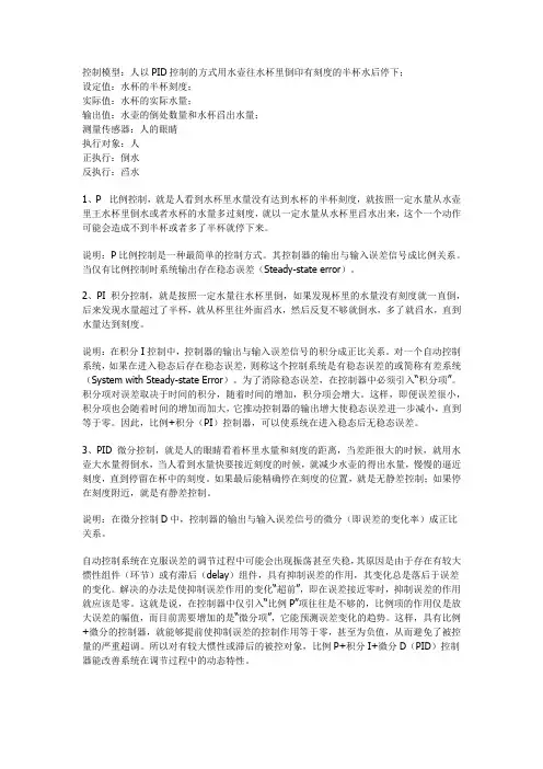
控制模型：人以PID控制的方式用水壶往水杯里倒印有刻度的半杯水后停下；设定值：水杯的半杯刻度；实际值：水杯的实际水量；输出值：水壶的倒处数量和水杯舀出水量；测量传感器：人的眼睛执行对象：人正执行：倒水反执行：舀水1、P 比例控制，就是人看到水杯里水量没有达到水杯的半杯刻度，就按照一定水量从水壶里王水杯里倒水或者水杯的水量多过刻度，就以一定水量从水杯里舀水出来，这个一个动作可能会造成不到半杯或者多了半杯就停下来。

说明：P比例控制是一种最简单的控制方式。

其控制器的输出与输入误差信号成比例关系。

当仅有比例控制时系统输出存在稳态误差（Steady-state error）。

2、PI 积分控制，就是按照一定水量往水杯里倒，如果发现杯里的水量没有刻度就一直倒，后来发现水量超过了半杯，就从杯里往外面舀水，然后反复不够就倒水，多了就舀水，直到水量达到刻度。

说明：在积分I控制中，控制器的输出与输入误差信号的积分成正比关系。

对一个自动控制系统，如果在进入稳态后存在稳态误差，则称这个控制系统是有稳态误差的或简称有差系统（System with Steady-state Error）。

为了消除稳态误差，在控制器中必须引入“积分项”。

积分项对误差取决于时间的积分，随着时间的增加，积分项会增大。

这样，即便误差很小，积分项也会随着时间的增加而加大，它推动控制器的输出增大使稳态误差进一步减小，直到等于零。

因此，比例+积分（PI）控制器，可以使系统在进入稳态后无稳态误差。

3、PID 微分控制，就是人的眼睛看着杯里水量和刻度的距离，当差距很大的时候，就用水壶大水量得倒水，当人看到水量快要接近刻度的时候，就减少水壶的得出水量，慢慢的逼近刻度，直到停留在杯中的刻度。

如果最后能精确停在刻度的位置，就是无静差控制；如果停在刻度附近，就是有静差控制。

说明：在微分控制D中，控制器的输出与输入误差信号的微分（即误差的变化率）成正比关系。

自动控制系统在克服误差的调节过程中可能会出现振荡甚至失稳，其原因是由于存在有较大惯性组件（环节）或有滞后（delay）组件，具有抑制误差的作用，其变化总是落后于误差的变化。