Abundance Analyses of Field RV Tauri Stars, VI An Extended Sample
- 格式:pdf
- 大小:445.25 KB
- 文档页数:42
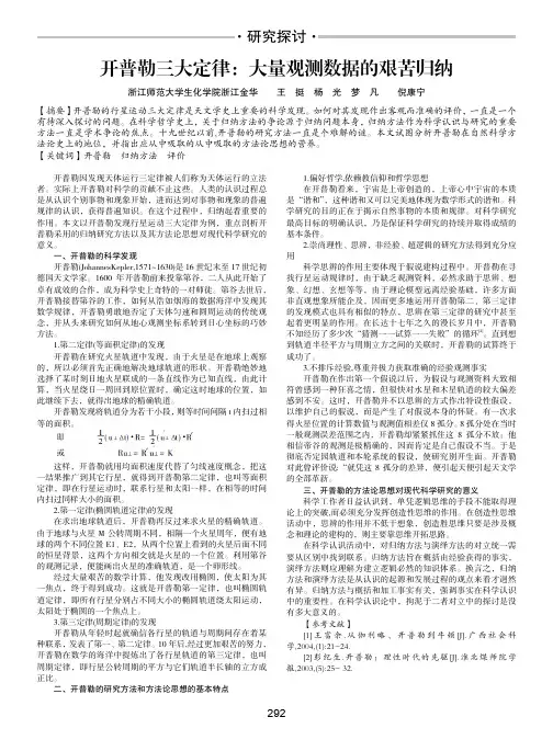
·研究探讨·292开普勒三大定律:大量观测数据的艰苦归纳浙江师范大学生化学院浙江金华 王 挺 杨 光 梦 凡 倪康宁【摘要】开普勒的行星运动三大定律是天文学史上重要的科学发现。
如何对其发现作出客观而准确的评价,一直是一个有待深入探讨的问题。
在科学哲学史上,关于归纳方法的争论源于归纳问题本身,归纳方法作为科学认识与研究的重要方法一直是学术争论的焦点。
十九世纪以前,开普勒的研究方法一直是个难解的谜。
本文试图分析开普勒在自然科学方法论史上的地位,并指出应从中吸取的从中吸取的方法论思想的营养。
【关键词】开普勒 归纳方法 评价开普勒因发现天体运行三定律被人们称为天体运行的立法者。
实际上开普勒对科学的贡献不止这些。
人类的认识过程总是从认识个别事物和现象开始,进而达到对事物和现象的普遍规律的认识,获得普遍知识。
在这个过程中,归纳起着重要的作用。
本文以开普勒发现行星运动三大定律为例,重点剖析开普勒采用的归纳研究方法以及其方法论思想对现代科学研究的意义。
一、开普勒的科学发现开普勒(JohannesKepler,1571~1630)是16世纪末至17世纪初德国天文学家。
1600年开普勒前来投靠第谷,二人从此开始了卓有成效的合作,成为科学史上奇特的一对师徒。
第谷去世后,开普勒接替第谷的工作,如何从浩如烟海的数据海洋中发现其数学规律,开普勒勇敢地否定了天体匀速和圆周运动的传统观念,并从头来研究如何从地心观测坐标系转到日心坐标的巧妙方法。
1.第二定律(等面积定律)的发现开普勒在研究火星轨道中发现,由于火星是在地球上观察的,所以必须首先正确地解决地球轨道的形状。
开普勒绝妙地选择了某时刻日地火星联成的一条直线作为已知直线,由此计算,当火星绕日一周回到原位置时,确定这时地球的位置,如此继续下去,就得出地球的精确轨道。
开普勒发现将轨道分为若干小段,则等时间间隔t 内扫过相等的面积。
这样,开普勒就用均面积速度代替了匀线速度概念,把这一结果推广到其它行星,就得到开普勒第二定律,也叫等面积定律,即在行星运动时,联系行星和太阳一样,在相等的时间内扫过同样大小的面积。
天文算法译著—许剑伟和他的译友第 1章注释与提示第 2章关于精度第 3章插值第 4章曲线拟合第 5章迭代第 6章排序第 7章儒略日第 8章复活节日期第 9章力学时和世界时第10章地球形状第11章恒星时与格林尼治时间第12章坐标变换第13章视差角第14章升、中天、降第15章大气折射第16章角度差第17章行星会合第18章在一条直线上的天体第19章包含三个天体的最小圆第20章岁差第21章章动及黄赤交角第22章恒星视差第23章轨道要素在不同坐标中的转换第24章太阳位置计算第25章太阳的直角坐标第26章分点和至点第27章时差第28章日面计算第29章开普勒方程第30章行星轨道要素第31章行星位置第32章椭圆运动第33章抛物线运动第34章准抛物线第35章一些行星现象的计算第36章冥王星第37章行星的近点和远点第38章经过交点第39章视差修正第40章行星圆面被照亮的比例及星等第41章火星物理表面星历计算(未译) 第42章木星物理表面星历计算(未译) 第43章木星的卫星位置(未译)第44章土星环(未译)第45章月球位置第46章月面的亮区第47章月相第48章月亮的近地点的远地点第49章月亮的升降交点第50章月亮的最大赤纬第51章月面计算第52章日月食第53章日月行星的视半径第54章恒星的星等第55章双星第56章日晷的计算备注译者说明原著《天文算法》天文算法天文算法 (1)前言 (1)第一章注释与提示 (1)第二章关于精度 (7)第三章插值 (16)第四章曲线拟合 (29)第五章迭代 (40)第六章排序 (47)第七章儒略日 (51)第八章复活节日期 (58)第九章力学时和世界时 (61)第十章地球形状 (65)第十一章恒星时与格林尼治时间 (70)第十二章坐标变换 (75)第十三章视差角 (80)第十四章天体的升、中天、降 (83)第十五章大气折射 (87)第十六章角度差 (89)第十七章行星会合 (97)第十八章在一条直线上的天体 (99)第十九章包含三个天体的最小圆 (101)第二十章岁差 (104)第二十一章章动及黄赤交角 (112)第二十二章恒星视差 (116)第二十三章轨道要素在不同坐标中的转换 (125)第二十四章太阳位置计算 (129)第二十五章太阳的直角坐标 (137)第二十六章分点和至点 (143)第二十七章时差 (148)第二十八章日面计算 (153)第二十九章开普勒方程 (157)第三十章行星的轨道要素 (172)第三十一章行星位置 (175)第三十二章椭圆运动 (178)第三十三章抛物线运动 (193)第三十四章准抛物线 (197)第三十五章一些行星现象的计算 (201)第三十六章冥王星 (211)第三十七章行星的近点和远点 (215)第三十八章经过交点 (221)第三十九章视差修正 (224)第四十章行星圆面被照亮的比例及星等 (230)第四十一章火星物理表面星历计算(未译) (234)第四十二章木星物理表面星历计算(未译) (234)第四十三章木星的卫星位置(未译) (234)第四十四章土星环(未译) (234)第四十五章月球位置 (235)第四十六章月面被照亮部分 (243)第四十七章月相 (246)第四十八章月亮的近地点和远地点 (252)第四十九章月亮的升降交点 (259)第五十章月亮的最大赤纬 (261)第五十一章月面计算 (265)第五十二章日月食 (273)第五十三章日月行星的视半径 (284)第五十四章恒星的星等 (286)第五十五章双星 (289)后记 (1)前言十分诚恳地感谢许剑伟和他的译友!在此我作一个拱手。
0254-6124/2021/41(2)-310-10Chin. J. Space Sci.空间科学学报ZHANG Jiawen, ZHENG Jianhua, WANG Youliang, LI Mingtao. Trajectory design for solar approaching detection mission using multiple resonant gravity assists of the Venus (in Chinese). Chin. J. Space Sci., 2021, 41(2): 310-319. D01:10.11728/cjss2021.02.310基于金星共振借力的太阳抵近探测任务轨道设计张佳文1>2郑建华M王有亮1李明涛w1(中国科学院国家空间科学中心北京100190)2(中国科学院大学北京100049)摘要对于太阳抵近探测任务,从地球直接发射探测器至太阳附近需要消耗巨大能量,通过多次金星借力飞行,可有效降低地球发射能量C3及中途变轨的燃料消耗.本文研究基于金星共振借力的太阳抵近探测任务轨道优化 设计,建立了连续共振借力和混合共振借力的转移轨道优化设计模型,并针对2025—2028年的发射窗口开展太阳 抵近探测任务轨道优化设计.仿真结果表明,相比连续共振借力,混合共振借力可以有效缩短太阳抵近探测任务的 轨道转移时间,对于地球发射能量C3和中途变轨燃料消耗的影响未见明显的规律性,能量降低与序列中的共振比 相关.关键词太阳抵近探测,共振借力,轨道设计中图分类号V412T rajectory D esign for Solar A pproaching D etectio n M ission U sin g M ultiple R eson an t G ravityA ssists of th e V enusZHANG Jiawen1,2ZHENG Jianhua1,2WANG Youliang1LI Mingtao1-2'[^National Space Science Center,Chinese Academy of Sciences, Beijing100190)2{University of Chinese Academy of Sciences, Beijing100049)A b s t r a c t T o a p p r o a c h c l o s e t o t h e S u n,d i r e c t l a u n c h f r o m t h e E a r t h c o s t s a lot o f e n e r g y,w h i c hc a n b e e f f e c t i v e l y r ed u ce d b y t h e g r a v i t y a s s i s t of t h e V e n u s.I n t h i s p a p e r,i n t e r p l a n e t a r y t r a n s f e rt r a j e c t o r i e s w i t h m u l t i p l e r e s o n a n t g r a v i t y a s s i s t s o f t h e V e n u s a r e d e s i g n e d f o r a s o l a r a p p r o a c h i n gd e t e c t i o n m i s s i o n.A n d d e s i g n m o d e l s f o r t h e t r a j e c t o r i e s w i t h c o n t i n u o u s r e s o n a n t g r a v i t y a s s ists,a s w e l l a s r e s o n a n t a n d n o n-r e s o n a n t g r a v i t y a s s i s t s c o mb i n e d a r e b u i l t.A m i s s i o n l a u nc h ed be t w e e n2025 a n d 2028 is s t u d i e d.T h e s t u d y s h o w s t h a t, c o m p a r e d w i t h t r a j e c t o r y w i t h c o n t i n u o u s r e s o n a n tg r a v i t y assis t s,t r a j e c t o r y w i t h r e s o n a n t a n d n o n-r e s o n a n t g r a v i t y a s s i s t s c o m b i n e d is u s e f u l f o rr e d u c i n g t r a n s f e r t i m e o f s o l a r a p p r o a c h i n g d e t e c t i o n m i s s i o n.A n d its i m p a c t o n t h e e n e r g y c o s t is n o t u n i v e r s a l,w h i c h is r e l a t e d t o t h e r e s o n a n c e r a t i o i n t h e t r a j e c t o r y.K e y w o r d s S o l a r a p p r o a c h i n g d e t e c t i o n,R e s o n a n t g r a v i t y assist, T i'a j e c t o r y d e s i g n2019-11-27收到原稿,2020-09-13收到修定稿E-mail: ***********************〇引言深空探测任务飞行时间长,转移所需能置大,为 了节约发射成本和降低燃料消耗,很多深空探测任务 都采用借力飞行技术.借力飞行(gravity assist /fly - by )技术是指设计深空探测器轨道经过天体附近,利 用其引力进行加速、减速或转向.为实现连续借力, 通过设计借力参数,使得探测器借力后与借力天体 之间形成共振轨道的借力飞行技术称为共振借力飞 行(resonant gravity assist ) •截至目前,国际上很多深空探测任务都采用了借 力飞行技术,其中应用共振借力飞行技术的任务中比 较典型的有:伽利略号木星探测任务(Galileo ),采用 金星地球-地球借力(VEEGA )序列,探测器经第一 次地球借力后,其轨道周期与地球轨道周期呈2 :1 关系;帕克太阳探测器(Parker Solar Probe , PSP ), 采用7次金星借力(V 7GA )序列,转移轨道中设计 了 3次共振借力,分别实现探测器与金星轨道周期 成2:3, 1 :2, 3:7的比例关系.共振借力飞行主要应用于多次借力的飞行任务 中,主要设计目标是:将探测器借力后的轨道周期与 借力天体轨道周期设计成一简单的整数比,为下一次 借力设计提供便利.对于太阳抵近探测任务,如果直接将探测器发射 到远日点距离为1 AU (A U 为天文单位),近日点距离 为10风(i ?s 为太阳半径)的大椭圆轨道上,需要的 发射能M 高达437km 2f -2,目前的运载火箭尚未达 到这个发射能力,因此通过借助行星的引力降低发射 能量是必由之路.对于太阳抵近探测任务,20世纪末即有研究提 出通过木星借力将探测器转移至距离太阳4〜15艮 的任务概念I 1#.由于科学研究非常关注太阳极区位 置,因此设计探测器经木星借力后偏离黄道面,沿高 倾角轨道飞向太阳,飞行时间为3.5〜4a .这也是帕克 太阳探测任务早期的轨道方案.但是此方案中探测 器飞至木星的路程远,对其热控与能源系统要求非常 高,并且探测器最终目标轨道的周期长达4年,使得 有限的任务周期内可对太阳进行就位探测的时间极 短,有研究提出了 7次金星借力的轨道转移方案1气 探测器预计7年后转移至近日点距离为9.8凡、周期 为88 d 的观测轨道上,对太阳进行就位观测.实际上,SukhanovW 在1999年即已提出通过内张佳文等:基于金星共振借力的太阳抵近探測任务轨道设计行星借力将探测器转移至太阳附近的轨道方案,并设计了发射窗口在2002年,通过金星、地球、火星的 借力将探测器送至近H 点距离为15〜30亿的轨道方 案,转移时间约为4.5〜13.3a .近年来中国也开展了太阳抵近探测任务的预先 研究.本文通过建立连续共振借力轨道和混合共振 借力轨道的优化设计模型,针对2025年至2028年 间发射,任务时长小于10年并最终转移至距太阳小 于10亿的太阳抵近探测任务,设计了通过金星共振 借力实现转移的轨道方案,得到混合共振借力轨道比 连续共振借力轨道更节省转移时间的结论.1轨道动力学基础深空探测器在太阳系内运动时会受到太阳和行星的引力,这是一个非线性多体系统.在轨道初步设 计阶段,为了简化计算,通常利用圆锥曲线拼接法设 计探测器飞行轨迹,认为探测器在行星引力影响球之 外时只受到太阳引力作用,其轨道为日心轨道;而运 行在行星引力影响球之内时,仅考虑此行星的引力, 探测器沿行星中心双曲线轨道运动间.考虑到探测器在日心飞行段的时间和空间都比 在行星附近飞行时大得多,因而在计算行星借力飞行 时,将行星借力飞行近似为探测器在H 心惯性系下获 得的一个瞬时速度增量,不考虑其位置变化,假设借 力瞬间完成,这种近似模型称为行星借力飞行等效脉 冲模型间.1.1借力飞行在借力飞行等效脉冲模型中,认为借力飞行瞬间 探测器的日心位置与借力行星的日心位置相同,并 且借力飞行前后探测器的H 心位置不变.探测器进 入与离开行星引力影响球时,相对于行星的速度分 别为双曲线进入剩余速度和双曲线离开剩余速 度 <,即W 二= v _-v p ,v -^=v + ~ Up.(1)式中,W 与…+分别为探测器借力前后的日心速度, %为借力飞行时行星的日心速度.借力飞行过程中, 如果探测器不进行主动轨道机动,其相对于行星沿双 曲线轨道运动,双曲线进入剩余速度与离开剩余速度 相等,即满足^〇〇 == I k ill -(2)311312Chin. J. Space Sci.空间科学学报2021,41(2)探测器借力飞行的轨迹如图1所示,根据双曲在该坐标系下,探测器的双曲线剩余速度可表示为 线几何关系,双曲线速度偏转角由下式确定:([J= 2 arcsin--—~.(3)M p+ruvio式中,rh为双曲线轨道近星点半径,叫为借力行星 的中心引力系数.为计算借力后探测器的日心速度,建立以借力行 星为中心的借力飞行坐标系如图2所示,坐标 系原点P选在借力行星中心,i轴沿双曲线进入剩 余速度方向,/c轴选取垂直于双曲线进入剩余速 度心与借力行星日心速度所决定的平面方向,j 轴与i轴和fc轴构成右手坐标系,三轴的单位矢童i,J’.fc分别表示为v t〇 =^(s i n5cos ipk+sin<5sin(pj +cos S i).(6)式中,p为在jA:平面上的投影与A•轴的夹角,取 值范围为[〇,2t t).由于借力飞行过程中探测器双曲线轨道的近星 点与行星表面距离不能小于安全高度/ipm in (事先设 定).相应地,J存在最大值<5max,即<5m ax= 2 arcsin—^P,---厂^.(7)"p+(*^p+"p m i n)U〇〇式中,&为借力行星的半径.对于无机动的借力飞行,已知双曲线进入剩余速 度通过设计借力高度~和借力角度a可以得 到借力后探测器的双曲线离开剩余速度w+.由于探 测器以速度离开借力行星时不一定能够到达下一个目标位置,通常需要在借力飞行前后施加速度脉 冲进行轨道修正.1.2共振借力对于能量要求高的深空探测任务.1次借力飞行 提供给探测器的能量有限.为更好地发挥借力飞行 效果,可以设计连续利用同一颗行星进行多次借力飞 行,其中将借力飞行设计为共振借力是便捷有效的方法之一.假设借力后探测器与借力行星的轨道周期比值 为# (共振轨道中周期比也称共振比),则有l=N.(8)图1借力飞行双曲线轨道Fig. 1G ravity assist hyperbolic trajectory图2借力飞行坐标系Fig. 2 G ravity assist frame of reference 式中,r s与r p分别为探测器与借力行星轨道周期.将行星日心速度投影在借力飞行坐标系下,结合 式(6)可以得到借力后探测器的日心速度,即V p =V p aji+V p yJ.+(9)= ivpz 4- v〇〇 s i n S c o s(r p y + u〇〇 s i n(5 s i n w)j+(vP x+v〇〇cos6)i.(10)结合二体运动能量守恒关系,整理得到如下关系:—(1 - W2/3) - 2i;p:d cos(5 - ^其中.M为太阳中心引力常数,%为借力行星轨道半张佳文等:基于金星共振借力的太阳抵近探測任务轨道设计313长轴量为R ==\!vi^-1-v^y sin((/?6), 0 =arctan-^1.^Py(12)记作R=Q-(13)\/V l z+vly则有Q =sin((/?H-6).(14)因此,探测器借力后能够与借力行星形成共振轨道的 充要条件为{t〇, A t i,A v i x,A v i y,A v X z,r p i, iVi, • • •, 'j^^(n —l)x*l)y 5 ^^(n—l)z i ^*p(n—1) i / •N(n_i、,rpn,<p n J(17)式中,妃为地球出发时间;A h为地球出发至第一次 金星借力的转移时间;A%,分别为每次 共振借力前在速度三个方向施加的速度增量;r*pi为 借力高度;为第n次借力的偏转角度;况为共振借力要实现的共振比,具体形式为Ni = Tsi : Tyenus = K i'.J i,(18)-1 彡 1.相应地.<P ={arcsin Q—0,sn —arcsinQ—9.J1,1;1—1,—1 彡Q彡0.(15)(16)观察式(l4),Q中含有借力角度A联系 式(11)〜(13),Q的表达式中含有借力高度决定的 角度<5,因此在满足共振借力的充要条件下,这两个 角度中只要确定一个,另一个即可确定,这说明在设 计共振借力飞行时,给定共振比与借力高度(偏转角 度6随之确定),借力角度v即随之确定.其中,Ts i为探测器轨道周期,r venus为金星轨道周期. 相应地,第U欠共振借力至第(i+ 1)次借力之间的 转移时间为A<(i+1) =Ki ■T venus- (19)根据前文分析,前(n- 1)次共振借力只需设计 借力高度与共振比即可完成,第n次非共振借力需 要通过借力高度与借力角度共同设计.在优化计算中.行星的位置由行星星历表得到,即P i=W{^P planet,i? ^i)*(20)其中,=亡0 +〉:A tj.(21)j-=i2轨道优化模型与方法在此模型的轨道设计中,希望得到低能耗转移轨 道,对应的优化目标为2.1连续共振借力轨道优化模型考虑连续共振借力(n- 1)次,最后一次非共振 借力的VnG A轨道模型⑵如图3所示.为了在共振借力后实现给定共振比,在每次共振 借力前施加速度脉冲Aw,修正轨道.对应的决策变m i n :/x(X)= C3=||V d e p - V e a r t h||2,(22) m i n :f2(X) = \/Avl +i=1 (23) Resonant orbit .Lambertd•一•Resonant orbitTime +A/1+A/2(/^l Tvenus )+厶'(,,-1、(尺("-2}厂v e n u s)(K(n~i)7\.e n图3连续共振借力轨道模型Fig. 3 Continuous resonant gravity assists trajectory model314Chin. J. Space Sci.空间科学学报2021,41(2)min:/3(X) =PT n=an(l-e n).(24)式中,V dep为探测器发射时的日心速度:v earth为发射时地球的日心速度;C3为地球发射能量;a…,e…,分别为最后一次借力后探测器轨道的半长轴、偏 心率和近H点距离.约束条件为^pi ^m in•(25)其中,rpmin为借力髙度约束.2.2混合共振借力轨道优化模型考虑共振借力与非共振借力交替,最后再补充1次非共振借力,其V”G A轨道模型如图4所示,其 中n为奇数,相应的轨道包含(n- 1)/2次共振借力 和(n+1)/2次非共振借力.同样地,对于共振借力,为了在借力后实现给定 共振比,每次借力前施加脉冲机动Aw,修正轨道.对 应的决策变量为而第H欠非共振借力(i为偶数)至第(i+1)次借力之 间的转移时间A~+1)需要通过设计给出,例如/^3, A亡5’…,这里借力飞行的设计方法与连续共振借力轨道 设计模型中相同,不同的是,需要通过求解Lambert 问题对非共振借力与下一次借力之间的轨道进行拼 接,为了匹配能量,需要在每一次非共振借力后施加 速度脉冲,其将与共振借力前施加的速度脉冲共同作 为优化目标.在仿真计算中,行星位置获取方法及约束条件与 连续共振借力轨道设计模型中相同,由于此模型希望 得到低能耗快速转移轨道,对应的优化目标在前者模 型的基础上,多出一个转移时间的目标函数,即nmin:f4{X) =y^A tj.(29)i=l2.3优化方法这里的优化计算采用差分进化算法(DifferentialX = {<〇,Aw lx,Auiy,^*p2)^21i^p(n—1)i^(n—1)5^p m}• (26)式中,M为地球出发时间;为地球出发至第1次 金星借力的转移时间;A〜,A r iy,分别为每次共振借力前在速度三个方向施加的速度脉冲;r pi为借力高度:为非共振借力的角度:况为共振借力 要实现的共振比,即Nt=Tsi:T ven u s= K i\J l.(27)其中,r st为探测器轨道周期,r venus为金星轨道周期. 相应的第i次共振借力(i为奇数)至第(i+1)次非 共振借力之间转移时间为A t(i+1) =A^Tvenus-(28)LambertResonant orbit+A/i+A/2E v o l u t i o n A l g o r i t h m. D E).此算法是基于群体的启发 式搜索算法,进化流程中包括变异、交叉和选择操作.D E算法采用浮点数矢量进行编码生成种群中的个 体,其寻优过程的步骤为:①从父代中选择2个个体进行矢量带权做差生成差分矢童,选择另一个体与差 分矢董求和生成实验个体,这一步为变异操作;②对 父代个体与实验个体进行交叉操作,生成新的子代个 体;③在父代个体与子代个体之间进行选择操作,将 符合要求的个体保留到下一代.由于D E算法新颖的变异操作,其在迭代初期具有较强的全局搜索能力,而在迭代后期具有较强的局 部搜索能力,相比其他同类方法具有待定参数少、不 易陷入局部最优且收敛速度快%的优点.在数值仿真中应用差分进化算法191时,由于决—:------------------------------------------------------►Time+A<3…+A V…Lambert Lambert書…_A(K] T venu s )i^(n~2) T'v e n u s)图4混合共振借力轨道模型Fig. 4 R esonant and non-resonant gravity assists combined trajectory model策变量X包含的变量个数Z较大,设置种群中个体 数量为5〇Z〜60/,最大迭代代数为1500丨〜2000Z;变 异操作权重设置为0.75,交叉率取为0.99.对于优 化模型中的多个优化目标,通过加权的方式进行处 理[1Q1.在连续共振借力轨道优化模型的仿真计算 中,优化函数设置为n—1____________________ F(X)=h C3 + k2Y,^v f x ++Avfz +i=lk3Prn-(30)混合共振借力轨道优化模型仿真计算中,优化函数设 置为71—1____________________________ F(X) =^03 + ^^2\/^l ++2=1nhPrn +k4y^yA tj.(31)i=\其中,h,fc2,fc3,A;4为权重系数,在D E算法执行过 程中取值如下:张佳文等:基于金星共振借力的太阳抵近探測任务轨道设计k\ = ^1000,、10,◦3〉^*3m a x;^3 ^^3 m ax •(32)k2 =1000,(33)ks=<,1000,‘ 1,Pm>Prnw’、Prn4Prnw(34)^1000,〉:>Tm a.x\A:4 =<i=ln(35) 1,〉:i ^^rnax*其中,c3max为仿真中设置的最大发射能量值,p r_为探测器最终抵达轨道的近日点距离最大值,Tm a x 为探测器最大转移时间.这样设置权重系数后,对不 符合轨道设计要求的解进行惩罚,进而自动舍弃.3数值仿真3.1任务分析从地球出发的探测器可以通过两种霍曼转移方 式直接转移至远日点在金星轨道处、近日点距离为 10凡的大椭圆轨道上,其消耗的能量非常大,具体 参数列于表1,转移轨道如图5所示.从表1中的数据可以看出,探测器直接转移消耗能量巨大,需借助行星引力降低发射能量和转移过程 中的燃料消耗.对于太阳抵近探测任务,探测器飞向 内太阳系,内行星的位置与轨道周期比外行星更适合 此任务.对比水星、金星和地球:水星的质量偏小,单 次借力对探测器轨道改变的能力较弱;金星质量略小 于地球,而轨道周期更短,对于多次借力的转移方案 更具有时间优势,因此选择金星作为借力天体.当探测器从地球出发,为了得到通过1次金星 借力可使其到达的轨道近日点距离与发射能量的关 系,在2025年的发射窗口内搜索V G A序列,得到的 优化结果如图6所示.由图6可以看到,若要探测器以可接受的发射 能量转移到近日点距离小于1〇凡的观测轨道上,1次金星借力远远不够.必须进行多次金星借力.接下 来分析并设计金星共振借力轨道.从单次金星借力V G A序列的计算结果可以得 到,当发射能量C3为150km2_S_2时,1次金星借力 后探测器的轨道近日点距离为33.7386亿,轨道半长 轴为0.7123av en u s (ave_为金星的轨道半长轴),探315表1霍曼转移能量消耗Table 1 Hohmann transfer’s energyconsumption转移方式1转移方式2地球发射能量437.0768 6.2269C3/(k m2-s"2)A v2/(k m-s_1) 1.602125.556316C h in. J. Sp a ce S c i .空间科学学报2021,41(2)测器与金星轨道周期比为0.6012.而对于近日点距 离为10凡、远日点距离为l a venus 的轨道,其轨 道半长轴为〇.5314a venus,相应与金星轨道周期比 为 0.3882.如果将发射能量C 3约束在150km 2.S _2左右, 为了充分发挥金星借力的作用,在第一次借力后,限 制探测器与金星的轨道周期比不大于2:3 (0.6667); 而最后一次共振借力后探测器与金星周期比至少 为3:8 (0.375),这样,最多需要补充1次借力飞行 探测器轨道的近日点距离即可降低至10艮以内.由于存在最小借力高度的约束,单次借力对探测 器轨道改变的程度有限,因此共振借力可实现的共 振比有限.在设计共振借力的共振比时,需同时考 虑借力时探测器的轨道能量以及此周期比对应的转 移时间是否合理.例如:探测器与金星的轨道周期 比为 2:3 (0.6667)时,二者飞行 2r v en u s (r v e n u s = 224.7d ,为金星公转周期)后即可相遇;当探测器与 金星周期比为5 :8 (0.625)时,二者需要飞行5 Tv e n u s 后才可以相遇.这两个例子中,虽然二者周期比值相fT 200 1 180 I160W0>| 140CU•g120c C OJ 1002628 3032 3436 38 4042 44 46Perigee radius//? s图6 V G A 地球发射能量与轨道近日点距离关系Fig. 6 Relationship between E a rth ’s launch energyand the o rb it’s perigee radius in VGAVGA近,但是所需飞行时间相差674d 左右.因此,为缩短 探测器的转移时间,在本文的仿真计算中,定义共振 比为尺:j (x : j = r s : r ven us ,r s 为探测器周期),仅 考虑尺< 5的情况.综上分析,设计共振借力轨道时.考虑采用表2 中的共振比.3.2仿真结果根据以上分析,针对太阳抵近探测任务,组合共 振比,分别设计金星连续共振借力轨道与混合共振借 力轨道.对2025年至2028年间采用不同飞行序列 飞向太阳的发射机会进行搜索.结合未来运载火箭 可能的发射能力,假设从地球出发时运载火箭可为探 测器提供的发射能量C 3最多为160km 2,S_2,目标轨 道为近日点距离小于10尾的日心椭圆轨道,约束任 务时间在10年以内.3.2.1连续共振借力轨道结果设计采用5次连续共振借力的V 6G A 轨道序列, 将不同共振比飞行序列得到的优化结果列于表3.表3中共振比序列为2 : 3, 4 : 7, 1 : 2, 4 : 9. 3 : 7 的轨道方案详细参数列于表4,轨道迹线如图7所示. 3.2.2混合共振借力轨道结果根据前文分析以及表3中的结果可以看出,共振 借力的共振比值直接决定了连续共振借力轨道方表2轨道设计中考虑的共振比T a b le 2R e s o n a n c e ra tio c o n s id e re din tr a j e c t o r y d e sig n共振比共振比(r s :7;enus)0.7 〜0.62 3 (0.6667),3:5 (0.6)0.6 〜0.547 (0.5714), 1:2 (0.5)0.5 〜0.449 (0.4444), 3:7 (0.4286), 2:5(0.4)0.4 〜0.338 (0.375)表3V 6G A 优化结果T a b le 3O p tim a l tr a je c to r ie s o f V 6G A共振比序列发射时间(UTC)发射能量C V (km 2.s-2)速度增量/(k m -s -1)近日点距离转移时间/a3:5, 4:7, 1:2, 4:9, 3:72026-08-08159.42940.82989.99289.34682:3, 4:7, 1 : 2, 4:9, 3:72026-08-06159.98950.40539.90978.75893:5, 4:7, 1 :2, 4:9, 2:52028-03-17159.9828 1.53338.78228.75742:3, 4:7, 1:2, 4:9, 2:52026-08-12145.82311.68958.86658.1379张佳文等:基于金星共振借力的太阳抵近探測任务轨道设计317日期速度增飞越 ______________________________借力后_____________________________(UTC) tt/f k m -s -1) 高度/k m半长轴/a venus周期/d 近日点距离/凡1金星2026-09-280.08854755.24900.7631149.8001 (2:3)34.70822金星2027-12-220.08531453.43540.6886128.3999 (4 : 7)26.85223金星2030-06-080.07581074.53210.6300112.3497 (1:2)20.18914金星2031-01-180.0883211.84210.582499.8663 (4 :9)14.46975金星2033-07-050.06721072.83960.568496.2996 (3:7)12.79316金星2035-05-10306.41520.544590.28369.9097表5V 7G A 优化结果T able 5O p tim al tr a je c to r ie s o f V 7G A共振比序列发射时间(UTC)发射能量C 3/(k m 2s -2)速度增量/(k m -s -1)近日点距离/Rs转移时间/a3:5, H, 1 :2, H, 3:7, H 2028-03-20159.99480.10879.99957.46952:3, H , 1 :2, H , 3:7, H 2026-08-03156.06020.00399.4716 6.24363:5, H, 1 :2, H, 2:5, H 2028-03-18159.9939 2.12519.2655 6.23332:3, H, 1:2, H, 2:5, H2028-03-19159.99292.04549.28445.6176案的转移时间.而V ^G A 轨道序列中含有共振比 为4 : 7与4 : 9的共振借力,对应的借力后的轨道段 需要4 r venus 的转移时间,如果将需要较长转移时间 的共振借力设计为非共振借力,则有希望获得总转移 时间相对更短的轨道方案.因此,改进V6G A 序列方 案,将共振比为4 : 7和4 : 9的共振借力替换成非共 振借力,并在第6次非共振借力后再补充1次金星 借力.设计为混合共振借力的V 7G A 序列.得到的优 化结果见表5,其中H 代表轨道中的非共振借力(除Fig. 7 Trajectory of V6GA 2:3, 4:7, 1:2, 4:9, 3:7最后一次借力外).将表5中借力序列为2 : 3, H , 1 : 2, H . 3 : 7, H 的轨道方案参数列于表6,其轨道迹线如图8所示. 3.2.3结果分析对比表3与表5中各方案的转移时间可以看到, 相比连续共振借力轨道模型的V6G A 轨道方案,混 合共振借力轨道模型的V7G A 轨道方案转移时间更 短,这是将转移时间长、共振比为4 : 7和4 :9的共 振借力替换为非共振借力的结果.图 8 V 7GA 2:3, H ,1:2, H ,3:7, H 轨道Fig. 8 Trajectory of V 7GA 2 :3, H, 1 : 2, H, 3 : 7, H表4V 6G A 序列2:3, 4:7, 1:2, 4:9, 3:7的轨道详细参数T ab le 4D e ta ile d tra jecto ry p a ra m eters o f V 6G A 2:3, 4:7, 1.2, 4:9, 3:7力星借行力数借次318Chin. J. Space Sci .空间科学学报 2021,41(2)0,2:3/3:5H 1:2 H 3:7/2:5Gravity assist sequence图10 V 7G A 中每次借力所需速度增量曲线Fig. 10 Delta-v needed of each gravityassist in V7GAGravity assist sequence图9 V 6G A 中每次借力所需速度增量曲线Fig. 9 Delta-v needed of each gravityassist in V6GA反而升高;并且在两种轨道模型中,前两个方案的速 度增量都比后两个方案的小.该现象主要是由共振比不同导致的,见图9和图10各转移方案中每次借 力施加的速度增M 曲线.在图9和图10中,绿色、蓝色线分别代表前两个 方案,红色、青蓝色线分别代表后两个方案.从曲线 的变化趋势可以看出,两种轨道模型中.后两种方案 均在第5次借力前施加较大的速度增量,占整段轨道 转移中所需速度增t t 的主要部分.这主要是因为后两 个方案中第5次借力后的共振比为2 : 5 (0.4),比前两 个方案中第5次借力后的共振比3 : 7 (0.4286)小,相 应地.探测器在借力后的轨道能M 低,而单次金星借 力降低探测器轨道能量的能力有限,因此需要探测器 自身施加额外的机动能量降低探测器的能量.因此, 共振比不同导致转移方案需要的速度增量存在差异.此外,对比图9和图10中的同色曲线可以看出, 用非共振借力替代共振比为4 : 7和4 : 9共振借力后:前两个方案第2, 3, 4, 5次借力所需速度增量都 有明显降低;后两个方案第2, 3, 4次借力所需速度 增请几乎不变,保持较低数值,第5次借力所需速度增键明显升高.分析出现这个现象的可能原因:前两个方案中, 在第5次借力前.即将探测器与金星的周期比降为 3 :7之前,探测器在同一位置以4:7, 1 :2, 4:9的共 振比序列降低能量,未能充分利用金星借力改变轨表 6 V 7G A 2:3, H , 1:2, H , 3:7, H 轨道详细参数T ab le 6D e ta ile d tr a je c to r y p aram eters o f V 7G A 2:3, H , 1 :2, H , 3:7, H借力次数行星日期(UTC)速度增飞越高度/km半长轴/a venus借力后 周期/d近日点距离/凡1金星2026-09-2704289.04150.7631149.7971 (2:3)35.19582金星2027-12-200.00181885.47610.6958130.401727.42633金星2028-07-050605.11090.6300112.3478 (1 :2)19.85504金星2029-02-140.00072116.44630.5915102.222815.46325金星2029-10-1003962.32550.568496.2982 (3 : 7)12.90366金星2031-08-150.00144506.37180.552292.213011.14127金星2032-10-312000.536488.28219.4716对比表3与表5中各方案所需速度增量可以发 现.将部分共振借力替换为非共振借力且增加1次非 共振借力后,前两个转移方案所需速度增M 大小有所 降低,而后两个方案所需速度增量大小非但没有降低--3:5, H, 1:2, H, 3:7, H2:3, H, 1:2,H, 3:7,H --3:5, H, 1:2, H, 2:5, H2:3, H, 1:2, H, 2:5, H--3:5,4:7, 1:2,4:9,3:72:3,4:7, 1:2,4:9, 3:7 3:5,4:7, 1:2,4:9,2:5 2:3,4:7, 1:2,4:9,2:5;• J ) /&V道能量,而调整共振比为4 : 7和4 :9的共振借力为 非共振借力后.优化得到了更加合适的借力方位与能 量降低顺序.金星的借力效果得到充分利用,降低了 速度增量需求;对于后两个方案,在第5次借力前,即 将探测器与金星的周期比降低为2:5之前,探测器 在同一位置以4 : 7, 1 : 2, 4 :9这样的共振比序列降 低轨道能M 比较合理,调整共振比为4 : 7和4 : 9的 共振借力为非共振借力后反而破坏了合适的借力方 位,并且导致在第5次借力前需要更多的机动能量 来调整轨道.结合上述分析可以看出:相比连续共振借力轨 道模型的V 6G A 轨道方案,混合共振借力轨道模型 的V 7G A 轨道方案转移时间更短,而对于地球发射 能量C 3与中途变轨所需速度增童的改变没有普遍 规律,中途变轨所需速度增量主要与借力序列中共振 比数值有关,对于一些共振比序列的轨道,混合共振 借力轨道可降低能量需求,而对于其他一些轨道,反 而需要消耗更多的能t t .4结论针对太阳抵近探测任务,提出利用金星多次共振借力的轨道设计方法,建立了连续共振借力轨道 与混合共振借力轨道优化设计模型,并针对2025年 至2028年的发射窗口,分别设计了连续共振借力的V 6G A 以及混合共振借力的V 7G A 轨道方案.研 究结论如下.(1) 太阳抵近探测任务中.多次金星借力可以降 低发射能量和转移途中变轨的燃料消耗.(2) 2〇25—2〇28年期间,在发射能量C 3不超过160km 2.s -2,转移时间不超过10年,最终轨道近 日点距离小于10亿的约束下,两种轨道方案的最优 序列分别为:2 :3, 4 : 7, 1:2, 4 :9, 3 :7 (V ®GA ,2026 年);2 :3, H ,1 :2, H ,3 : 7, H (V 7GA ,2026 年).(3) 2026 年 8 月 3 日发射的 V7GA 2 : 3, H , 1 :2, H ,3:7, H 轨道方案,探测器以156.06〇2km 2.s -2 的发射能董从地球出发,先后经过7次金星 借力,途中几乎不消耗变轨燃料(变轨速度增量 为0.0039km .s -1),飞行6.2476a 后,转移至近日点 距离为9.4716凡、周期为88.2821 d 的观测轨道上.张佳文等:基于金星共振借乃的太阳抵近探測任务轨道设计(4)相比连续共振借力轨道,混合共振借力轨道 可有效缩短太阳抵近探测任务的轨道转移时间,而对于地球发射能量C 3与中途变轨所需速度增量的改变 没有普遍规律.这与序列中的共振比有关.参考文献[1] GALEEV A A, VAISBERG O L, ZAKHAROV A V, et al.Project Ziolkovsky-Solar Probe mission concept [J]. Adv.Space Res., 1996, 17(3): 13-20[2] TSURUTANI B T, VAISBERG O L. The Solar Probe mission and comments on plasma wave observations [CJ//AIP Conference Proceeding. New York: AIP Press, 1996: 255[3] GUO Y. Trajectory design of Solar Probe+ using multiple Venus gravity assists [CJ//AIAA/AAS Astrodyna- mics Specialist Conference and Exhibit. Honolulu, Hawaii: American Institute of Aeronautics and Astronautics, 2008: 3029-3039[4] SUKHANOV A A. Close approach to Sun using gravity assists of the inner planets [J]. Acta Astron., 1999, 45: 177- 185[5] QIAO Dong. Study of Transfer Trajectory Design Method for Deep Space Exploration and Application to Small Body Exploration [D]. Harbin: Harbin Institute of Tech- nology, 2007 (乔栋.深空探测转移轨道设计方法研究及在小天 体探测中的应用[D].哈尔滨:哈尔滨工业大学,2007)[6] LI Junfeng, BAOYIN Hexi, JIANG Fanghua. Dynamics and Control of Interplanetary Flight [M]. Beijing: Ts-inghua University Press, 2〇14: 110-127 (李俊峰,宝音贺西, 蒋方华.深空探测动力学与控制[M ].北京:清华大学出版社,2014:110-127)[7] YUAN Jianping, ZHAO Yushan, TANG Geshi, et al. Spacecraft Deep Space Flight Trajectory Design [M]. Beijing: China Astronautic Publishing House, 2014: 59-76 (袁建平,赵育善,唐歌实,等.航天器深空飞行轨道设计[M ].北京:中国宇航出版社,2014:59-76)[8] HU Zhongbo. The Study of Differential Evolution Algorithm for the Function Optimization [D]. Wuhan: Wuhan University of Technology, 2006 (胡中波•差分演化券法及其在函数优化中的应用研究[D].武汉:武汉理工大学,2006)[9] Differential evolution (DE) for continuous function optimization (an algorithm by Kenneth Price and Rainer Storn) [OL]. [2019-10-10] http://wwwl.icsi.berkeley. edu/〜storn/code.html#tevc[10] LI Xiaoyu. Design and Optimization of Deep Space Trajectory on the Initial Design Stage [D]. Beijing: University of Chinese Academy of Sciences, 2012 (李小玉.深空探测轨 道的初始方案设计与优化[D].北京:中国科学院大学,2012)319。
参宿三英语介绍参宿三,也被称为猎户座ε星,是一颗位于猎户座星云的恒星。
以下是关于参宿三的详细英语介绍:Betelgeuse, also known as Alpha Orionis and officially designated as HD 39801, is a red supergiant star located in the constellation of Orion. It is one of the largest and most luminous stars known, with a diameter that is estimated to be between 600 to 850 times that of the Sun and a luminosity approximately 90,000 times greater than the Sun.Betelgeuse is a variable star, meaning its brightness changes over time. It is classified as a Mira variable, which means its brightness varies by a large amount, typically between magnitudes 0.5 and 1.6 over a period of approximately 420 to 540 days. The brightness variations are caused by convection cycles in the star's atmosphere, which affect the star's temperature and therefore its luminosity.Betelgeuse is thought to be in the later stages of its life, having already burned most of its hydrogen fuel. It is now believed to be in a phase of rapid evolution, expanding and becoming cooler as it ages. In the coming millions of years, it is likely to become even more luminous and expand further, possibly becoming a type II supernova.The name Betelgeuse is believed to come from the Arabic expression "al Gift al J桴us", which translates to "the armpit of the central one". This name likely refers to its position in the constellation of Orion, as it marks the hunter's shoulder on the left side. The name was later anglicized to "Betelgeuse", which is the name it is known by today.Betelgeuse is easy to spot in the night sky due to its brightness and location in one of the most recognizable constellations, Orion. With the help of a telescope or even good binoculars, it can be seen as a red star with a distinct orange hue. It is often included in astronomy observing guides due to its visibility and ease of identification.Betelgeuse is a remarkable example of the diverse and fascinating world of variable stars. Its brightness changes over time make it a challenge to study, but its unique properties also allow astronomers to better understand the complex processes that occur within stars as they evolve and change over time. Betelgeuse remains a fascinating subject for astronomers and amateur stargazers alike, offering a window into the grand tapestry of our universe.以上是对参宿三的详细介绍,希望对您有所帮助。
Observation of Gravitational Waves from a Binary Black Hole MergerB.P.Abbott et al.*(LIGO Scientific Collaboration and Virgo Collaboration)(Received21January2016;published11February2016)On September14,2015at09:50:45UTC the two detectors of the Laser Interferometer Gravitational-Wave Observatory simultaneously observed a transient gravitational-wave signal.The signal sweeps upwards in frequency from35to250Hz with a peak gravitational-wave strain of1.0×10−21.It matches the waveform predicted by general relativity for the inspiral and merger of a pair of black holes and the ringdown of the resulting single black hole.The signal was observed with a matched-filter signal-to-noise ratio of24and a false alarm rate estimated to be less than1event per203000years,equivalent to a significance greaterthan5.1σ.The source lies at a luminosity distance of410þ160−180Mpc corresponding to a redshift z¼0.09þ0.03−0.04.In the source frame,the initial black hole masses are36þ5−4M⊙and29þ4−4M⊙,and the final black hole mass is62þ4−4M⊙,with3.0þ0.5−0.5M⊙c2radiated in gravitational waves.All uncertainties define90%credible intervals.These observations demonstrate the existence of binary stellar-mass black hole systems.This is the first direct detection of gravitational waves and the first observation of a binary black hole merger.DOI:10.1103/PhysRevLett.116.061102I.INTRODUCTIONIn1916,the year after the final formulation of the field equations of general relativity,Albert Einstein predicted the existence of gravitational waves.He found that the linearized weak-field equations had wave solutions: transverse waves of spatial strain that travel at the speed of light,generated by time variations of the mass quadrupole moment of the source[1,2].Einstein understood that gravitational-wave amplitudes would be remarkably small;moreover,until the Chapel Hill conference in 1957there was significant debate about the physical reality of gravitational waves[3].Also in1916,Schwarzschild published a solution for the field equations[4]that was later understood to describe a black hole[5,6],and in1963Kerr generalized the solution to rotating black holes[7].Starting in the1970s theoretical work led to the understanding of black hole quasinormal modes[8–10],and in the1990s higher-order post-Newtonian calculations[11]preceded extensive analytical studies of relativistic two-body dynamics[12,13].These advances,together with numerical relativity breakthroughs in the past decade[14–16],have enabled modeling of binary black hole mergers and accurate predictions of their gravitational waveforms.While numerous black hole candidates have now been identified through electromag-netic observations[17–19],black hole mergers have not previously been observed.The discovery of the binary pulsar system PSR B1913þ16 by Hulse and Taylor[20]and subsequent observations of its energy loss by Taylor and Weisberg[21]demonstrated the existence of gravitational waves.This discovery, along with emerging astrophysical understanding[22], led to the recognition that direct observations of the amplitude and phase of gravitational waves would enable studies of additional relativistic systems and provide new tests of general relativity,especially in the dynamic strong-field regime.Experiments to detect gravitational waves began with Weber and his resonant mass detectors in the1960s[23], followed by an international network of cryogenic reso-nant detectors[24].Interferometric detectors were first suggested in the early1960s[25]and the1970s[26].A study of the noise and performance of such detectors[27], and further concepts to improve them[28],led to proposals for long-baseline broadband laser interferome-ters with the potential for significantly increased sensi-tivity[29–32].By the early2000s,a set of initial detectors was completed,including TAMA300in Japan,GEO600 in Germany,the Laser Interferometer Gravitational-Wave Observatory(LIGO)in the United States,and Virgo in binations of these detectors made joint obser-vations from2002through2011,setting upper limits on a variety of gravitational-wave sources while evolving into a global network.In2015,Advanced LIGO became the first of a significantly more sensitive network of advanced detectors to begin observations[33–36].A century after the fundamental predictions of Einstein and Schwarzschild,we report the first direct detection of gravitational waves and the first direct observation of a binary black hole system merging to form a single black hole.Our observations provide unique access to the*Full author list given at the end of the article.Published by the American Physical Society under the terms of the Creative Commons Attribution3.0License.Further distri-bution of this work must maintain attribution to the author(s)and the published article’s title,journal citation,and DOI.properties of space-time in the strong-field,high-velocity regime and confirm predictions of general relativity for the nonlinear dynamics of highly disturbed black holes.II.OBSERVATIONOn September14,2015at09:50:45UTC,the LIGO Hanford,W A,and Livingston,LA,observatories detected the coincident signal GW150914shown in Fig.1.The initial detection was made by low-latency searches for generic gravitational-wave transients[41]and was reported within three minutes of data acquisition[43].Subsequently, matched-filter analyses that use relativistic models of com-pact binary waveforms[44]recovered GW150914as the most significant event from each detector for the observa-tions reported here.Occurring within the10-msintersite FIG.1.The gravitational-wave event GW150914observed by the LIGO Hanford(H1,left column panels)and Livingston(L1,rightcolumn panels)detectors.Times are shown relative to September14,2015at09:50:45UTC.For visualization,all time series are filtered with a35–350Hz bandpass filter to suppress large fluctuations outside the detectors’most sensitive frequency band,and band-reject filters to remove the strong instrumental spectral lines seen in the Fig.3spectra.Top row,left:H1strain.Top row,right:L1strain.GW150914arrived first at L1and6.9þ0.5−0.4ms later at H1;for a visual comparison,the H1data are also shown,shifted in time by this amount and inverted(to account for the detectors’relative orientations).Second row:Gravitational-wave strain projected onto each detector in the35–350Hz band.Solid lines show a numerical relativity waveform for a system with parameters consistent with those recovered from GW150914[37,38]confirmed to99.9%by an independent calculation based on[15].Shaded areas show90%credible regions for two independent waveform reconstructions.One(dark gray)models the signal using binary black hole template waveforms [39].The other(light gray)does not use an astrophysical model,but instead calculates the strain signal as a linear combination of sine-Gaussian wavelets[40,41].These reconstructions have a94%overlap,as shown in[39].Third row:Residuals after subtracting the filtered numerical relativity waveform from the filtered detector time series.Bottom row:A time-frequency representation[42]of the strain data,showing the signal frequency increasing over time.propagation time,the events have a combined signal-to-noise ratio(SNR)of24[45].Only the LIGO detectors were observing at the time of GW150914.The Virgo detector was being upgraded, and GEO600,though not sufficiently sensitive to detect this event,was operating but not in observational mode.With only two detectors the source position is primarily determined by the relative arrival time and localized to an area of approximately600deg2(90% credible region)[39,46].The basic features of GW150914point to it being produced by the coalescence of two black holes—i.e., their orbital inspiral and merger,and subsequent final black hole ringdown.Over0.2s,the signal increases in frequency and amplitude in about8cycles from35to150Hz,where the amplitude reaches a maximum.The most plausible explanation for this evolution is the inspiral of two orbiting masses,m1and m2,due to gravitational-wave emission.At the lower frequencies,such evolution is characterized by the chirp mass[11]M¼ðm1m2Þ3=5121=5¼c3G596π−8=3f−11=3_f3=5;where f and_f are the observed frequency and its time derivative and G and c are the gravitational constant and speed of light.Estimating f and_f from the data in Fig.1, we obtain a chirp mass of M≃30M⊙,implying that the total mass M¼m1þm2is≳70M⊙in the detector frame. This bounds the sum of the Schwarzschild radii of thebinary components to2GM=c2≳210km.To reach an orbital frequency of75Hz(half the gravitational-wave frequency)the objects must have been very close and very compact;equal Newtonian point masses orbiting at this frequency would be only≃350km apart.A pair of neutron stars,while compact,would not have the required mass,while a black hole neutron star binary with the deduced chirp mass would have a very large total mass, and would thus merge at much lower frequency.This leaves black holes as the only known objects compact enough to reach an orbital frequency of75Hz without contact.Furthermore,the decay of the waveform after it peaks is consistent with the damped oscillations of a black hole relaxing to a final stationary Kerr configuration. Below,we present a general-relativistic analysis of GW150914;Fig.2shows the calculated waveform using the resulting source parameters.III.DETECTORSGravitational-wave astronomy exploits multiple,widely separated detectors to distinguish gravitational waves from local instrumental and environmental noise,to provide source sky localization,and to measure wave polarizations. The LIGO sites each operate a single Advanced LIGO detector[33],a modified Michelson interferometer(see Fig.3)that measures gravitational-wave strain as a differ-ence in length of its orthogonal arms.Each arm is formed by two mirrors,acting as test masses,separated by L x¼L y¼L¼4km.A passing gravitational wave effec-tively alters the arm lengths such that the measured difference isΔLðtÞ¼δL x−δL y¼hðtÞL,where h is the gravitational-wave strain amplitude projected onto the detector.This differential length variation alters the phase difference between the two light fields returning to the beam splitter,transmitting an optical signal proportional to the gravitational-wave strain to the output photodetector. To achieve sufficient sensitivity to measure gravitational waves,the detectors include several enhancements to the basic Michelson interferometer.First,each arm contains a resonant optical cavity,formed by its two test mass mirrors, that multiplies the effect of a gravitational wave on the light phase by a factor of300[48].Second,a partially trans-missive power-recycling mirror at the input provides addi-tional resonant buildup of the laser light in the interferometer as a whole[49,50]:20W of laser input is increased to700W incident on the beam splitter,which is further increased to 100kW circulating in each arm cavity.Third,a partially transmissive signal-recycling mirror at the outputoptimizes FIG. 2.Top:Estimated gravitational-wave strain amplitude from GW150914projected onto H1.This shows the full bandwidth of the waveforms,without the filtering used for Fig.1. The inset images show numerical relativity models of the black hole horizons as the black holes coalesce.Bottom:The Keplerian effective black hole separation in units of Schwarzschild radii (R S¼2GM=c2)and the effective relative velocity given by the post-Newtonian parameter v=c¼ðGMπf=c3Þ1=3,where f is the gravitational-wave frequency calculated with numerical relativity and M is the total mass(value from Table I).the gravitational-wave signal extraction by broadening the bandwidth of the arm cavities [51,52].The interferometer is illuminated with a 1064-nm wavelength Nd:Y AG laser,stabilized in amplitude,frequency,and beam geometry [53,54].The gravitational-wave signal is extracted at the output port using a homodyne readout [55].These interferometry techniques are designed to maxi-mize the conversion of strain to optical signal,thereby minimizing the impact of photon shot noise (the principal noise at high frequencies).High strain sensitivity also requires that the test masses have low displacement noise,which is achieved by isolating them from seismic noise (low frequencies)and designing them to have low thermal noise (intermediate frequencies).Each test mass is suspended as the final stage of a quadruple-pendulum system [56],supported by an active seismic isolation platform [57].These systems collectively provide more than 10orders of magnitude of isolation from ground motion for frequen-cies above 10Hz.Thermal noise is minimized by using low-mechanical-loss materials in the test masses and their suspensions:the test masses are 40-kg fused silica substrates with low-loss dielectric optical coatings [58,59],and are suspended with fused silica fibers from the stage above [60].To minimize additional noise sources,all components other than the laser source are mounted on vibration isolation stages in ultrahigh vacuum.To reduce optical phase fluctuations caused by Rayleigh scattering,the pressure in the 1.2-m diameter tubes containing the arm-cavity beams is maintained below 1μPa.Servo controls are used to hold the arm cavities on resonance [61]and maintain proper alignment of the optical components [62].The detector output is calibrated in strain by measuring its response to test mass motion induced by photon pressure from a modulated calibration laser beam [63].The calibration is established to an uncertainty (1σ)of less than 10%in amplitude and 10degrees in phase,and is continuously monitored with calibration laser excitations at selected frequencies.Two alternative methods are used to validate the absolute calibration,one referenced to the main laser wavelength and the other to a radio-frequencyoscillator(a)FIG.3.Simplified diagram of an Advanced LIGO detector (not to scale).A gravitational wave propagating orthogonally to the detector plane and linearly polarized parallel to the 4-km optical cavities will have the effect of lengthening one 4-km arm and shortening the other during one half-cycle of the wave;these length changes are reversed during the other half-cycle.The output photodetector records these differential cavity length variations.While a detector ’s directional response is maximal for this case,it is still significant for most other angles of incidence or polarizations (gravitational waves propagate freely through the Earth).Inset (a):Location and orientation of the LIGO detectors at Hanford,WA (H1)and Livingston,LA (L1).Inset (b):The instrument noise for each detector near the time of the signal detection;this is an amplitude spectral density,expressed in terms of equivalent gravitational-wave strain amplitude.The sensitivity is limited by photon shot noise at frequencies above 150Hz,and by a superposition of other noise sources at lower frequencies [47].Narrow-band features include calibration lines (33–38,330,and 1080Hz),vibrational modes of suspension fibers (500Hz and harmonics),and 60Hz electric power grid harmonics.[64].Additionally,the detector response to gravitational waves is tested by injecting simulated waveforms with the calibration laser.To monitor environmental disturbances and their influ-ence on the detectors,each observatory site is equipped with an array of sensors:seismometers,accelerometers, microphones,magnetometers,radio receivers,weather sensors,ac-power line monitors,and a cosmic-ray detector [65].Another∼105channels record the interferometer’s operating point and the state of the control systems.Data collection is synchronized to Global Positioning System (GPS)time to better than10μs[66].Timing accuracy is verified with an atomic clock and a secondary GPS receiver at each observatory site.In their most sensitive band,100–300Hz,the current LIGO detectors are3to5times more sensitive to strain than initial LIGO[67];at lower frequencies,the improvement is even greater,with more than ten times better sensitivity below60Hz.Because the detectors respond proportionally to gravitational-wave amplitude,at low redshift the volume of space to which they are sensitive increases as the cube of strain sensitivity.For binary black holes with masses similar to GW150914,the space-time volume surveyed by the observations reported here surpasses previous obser-vations by an order of magnitude[68].IV.DETECTOR VALIDATIONBoth detectors were in steady state operation for several hours around GW150914.All performance measures,in particular their average sensitivity and transient noise behavior,were typical of the full analysis period[69,70]. Exhaustive investigations of instrumental and environ-mental disturbances were performed,giving no evidence to suggest that GW150914could be an instrumental artifact [69].The detectors’susceptibility to environmental disturb-ances was quantified by measuring their response to spe-cially generated magnetic,radio-frequency,acoustic,and vibration excitations.These tests indicated that any external disturbance large enough to have caused the observed signal would have been clearly recorded by the array of environ-mental sensors.None of the environmental sensors recorded any disturbances that evolved in time and frequency like GW150914,and all environmental fluctuations during the second that contained GW150914were too small to account for more than6%of its strain amplitude.Special care was taken to search for long-range correlated disturbances that might produce nearly simultaneous signals at the two sites. No significant disturbances were found.The detector strain data exhibit non-Gaussian noise transients that arise from a variety of instrumental mecha-nisms.Many have distinct signatures,visible in auxiliary data channels that are not sensitive to gravitational waves; such instrumental transients are removed from our analyses [69].Any instrumental transients that remain in the data are accounted for in the estimated detector backgrounds described below.There is no evidence for instrumental transients that are temporally correlated between the two detectors.V.SEARCHESWe present the analysis of16days of coincident observations between the two LIGO detectors from September12to October20,2015.This is a subset of the data from Advanced LIGO’s first observational period that ended on January12,2016.GW150914is confidently detected by two different types of searches.One aims to recover signals from the coalescence of compact objects,using optimal matched filtering with waveforms predicted by general relativity. The other search targets a broad range of generic transient signals,with minimal assumptions about waveforms.These searches use independent methods,and their response to detector noise consists of different,uncorrelated,events. However,strong signals from binary black hole mergers are expected to be detected by both searches.Each search identifies candidate events that are detected at both observatories consistent with the intersite propa-gation time.Events are assigned a detection-statistic value that ranks their likelihood of being a gravitational-wave signal.The significance of a candidate event is determined by the search background—the rate at which detector noise produces events with a detection-statistic value equal to or higher than the candidate event.Estimating this back-ground is challenging for two reasons:the detector noise is nonstationary and non-Gaussian,so its properties must be empirically determined;and it is not possible to shield the detector from gravitational waves to directly measure a signal-free background.The specific procedure used to estimate the background is slightly different for the two searches,but both use a time-shift technique:the time stamps of one detector’s data are artificially shifted by an offset that is large compared to the intersite propagation time,and a new set of events is produced based on this time-shifted data set.For instrumental noise that is uncor-related between detectors this is an effective way to estimate the background.In this process a gravitational-wave signal in one detector may coincide with time-shifted noise transients in the other detector,thereby contributing to the background estimate.This leads to an overestimate of the noise background and therefore to a more conservative assessment of the significance of candidate events.The characteristics of non-Gaussian noise vary between different time-frequency regions.This means that the search backgrounds are not uniform across the space of signals being searched.To maximize sensitivity and provide a better estimate of event significance,the searches sort both their background estimates and their event candidates into differ-ent classes according to their time-frequency morphology. The significance of a candidate event is measured against the background of its class.To account for having searchedmultiple classes,this significance is decreased by a trials factor equal to the number of classes [71].A.Generic transient searchDesigned to operate without a specific waveform model,this search identifies coincident excess power in time-frequency representations of the detector strain data [43,72],for signal frequencies up to 1kHz and durations up to a few seconds.The search reconstructs signal waveforms consistent with a common gravitational-wave signal in both detectors using a multidetector maximum likelihood method.Each event is ranked according to the detection statistic ηc ¼ffiffiffiffiffiffiffiffiffiffiffiffiffiffiffiffiffiffiffiffiffiffiffiffiffiffiffiffiffiffiffiffiffiffiffi2E c =ð1þE n =E c Þp ,where E c is the dimensionless coherent signal energy obtained by cross-correlating the two reconstructed waveforms,and E n is the dimensionless residual noise energy after the reconstructed signal is subtracted from the data.The statistic ηc thus quantifies the SNR of the event and the consistency of the data between the two detectors.Based on their time-frequency morphology,the events are divided into three mutually exclusive search classes,as described in [41]:events with time-frequency morphology of known populations of noise transients (class C1),events with frequency that increases with time (class C3),and all remaining events (class C2).Detected with ηc ¼20.0,GW150914is the strongest event of the entire search.Consistent with its coalescence signal signature,it is found in the search class C3of events with increasing time-frequency evolution.Measured on a background equivalent to over 67400years of data and including a trials factor of 3to account for the search classes,its false alarm rate is lower than 1in 22500years.This corresponds to a probability <2×10⁻⁶of observing one or more noise events as strong as GW150914during the analysis time,equivalent to 4.6σ.The left panel of Fig.4shows the C3class results and background.The selection criteria that define the search class C3reduce the background by introducing a constraint on the signal morphology.In order to illustrate the significance of GW150914against a background of events with arbitrary shapes,we also show the results of a search that uses the same set of events as the one described above but without this constraint.Specifically,we use only two search classes:the C1class and the union of C2and C3classes (C 2þC 3).In this two-class search the GW150914event is found in the C 2þC 3class.The left panel of Fig.4shows the C 2þC 3class results and background.In the background of this class there are four events with ηc ≥32.1,yielding a false alarm rate for GW150914of 1in 8400years.This corresponds to a false alarm probability of 5×10⁻⁶equivalent to 4.4σ.FIG.4.Search results from the generic transient search (left)and the binary coalescence search (right).These histograms show the number of candidate events (orange markers)and the mean number of background events (black lines)in the search class where GW150914was found as a function of the search detection statistic and with a bin width of 0.2.The scales on the top give the significance of an event in Gaussian standard deviations based on the corresponding noise background.The significance of GW150914is greater than 5.1σand 4.6σfor the binary coalescence and the generic transient searches,respectively.Left:Along with the primary search (C3)we also show the results (blue markers)and background (green curve)for an alternative search that treats events independently of their frequency evolution (C 2þC 3).The classes C2and C3are defined in the text.Right:The tail in the black-line background of the binary coalescence search is due to random coincidences of GW150914in one detector with noise in the other detector.(This type of event is practically absent in the generic transient search background because they do not pass the time-frequency consistency requirements used in that search.)The purple curve is the background excluding those coincidences,which is used to assess the significance of the second strongest event.For robustness and validation,we also use other generic transient search algorithms[41].A different search[73]and a parameter estimation follow-up[74]detected GW150914 with consistent significance and signal parameters.B.Binary coalescence searchThis search targets gravitational-wave emission from binary systems with individual masses from1to99M⊙, total mass less than100M⊙,and dimensionless spins up to 0.99[44].To model systems with total mass larger than 4M⊙,we use the effective-one-body formalism[75],whichcombines results from the post-Newtonian approach [11,76]with results from black hole perturbation theory and numerical relativity.The waveform model[77,78] assumes that the spins of the merging objects are alignedwith the orbital angular momentum,but the resultingtemplates can,nonetheless,effectively recover systemswith misaligned spins in the parameter region ofGW150914[44].Approximately250000template wave-forms are used to cover this parameter space.The search calculates the matched-filter signal-to-noiseratioρðtÞfor each template in each detector and identifiesmaxima ofρðtÞwith respect to the time of arrival of the signal[79–81].For each maximum we calculate a chi-squared statisticχ2r to test whether the data in several differentfrequency bands are consistent with the matching template [82].Values ofχ2r near unity indicate that the signal is consistent with a coalescence.Ifχ2r is greater than unity,ρðtÞis reweighted asˆρ¼ρ=f½1þðχ2rÞ3 =2g1=6[83,84].The final step enforces coincidence between detectors by selectingevent pairs that occur within a15-ms window and come fromthe same template.The15-ms window is determined by the10-ms intersite propagation time plus5ms for uncertainty inarrival time of weak signals.We rank coincident events basedon the quadrature sumˆρc of theˆρfrom both detectors[45]. To produce background data for this search the SNR maxima of one detector are time shifted and a new set of coincident events is computed.Repeating this procedure ∼107times produces a noise background analysis time equivalent to608000years.To account for the search background noise varying acrossthe target signal space,candidate and background events aredivided into three search classes based on template length.The right panel of Fig.4shows the background for thesearch class of GW150914.The GW150914detection-statistic value ofˆρc¼23.6is larger than any background event,so only an upper bound can be placed on its false alarm rate.Across the three search classes this bound is1in 203000years.This translates to a false alarm probability <2×10⁻⁷,corresponding to5.1σ.A second,independent matched-filter analysis that uses adifferent method for estimating the significance of itsevents[85,86],also detected GW150914with identicalsignal parameters and consistent significance.When an event is confidently identified as a real gravitational-wave signal,as for GW150914,the back-ground used to determine the significance of other events is reestimated without the contribution of this event.This is the background distribution shown as a purple line in the right panel of Fig.4.Based on this,the second most significant event has a false alarm rate of1per2.3years and corresponding Poissonian false alarm probability of0.02. Waveform analysis of this event indicates that if it is astrophysical in origin it is also a binary black hole merger[44].VI.SOURCE DISCUSSIONThe matched-filter search is optimized for detecting signals,but it provides only approximate estimates of the source parameters.To refine them we use general relativity-based models[77,78,87,88],some of which include spin precession,and for each model perform a coherent Bayesian analysis to derive posterior distributions of the source parameters[89].The initial and final masses, final spin,distance,and redshift of the source are shown in Table I.The spin of the primary black hole is constrained to be<0.7(90%credible interval)indicating it is not maximally spinning,while the spin of the secondary is only weakly constrained.These source parameters are discussed in detail in[39].The parameter uncertainties include statistical errors and systematic errors from averaging the results of different waveform models.Using the fits to numerical simulations of binary black hole mergers in[92,93],we provide estimates of the mass and spin of the final black hole,the total energy radiated in gravitational waves,and the peak gravitational-wave luminosity[39].The estimated total energy radiated in gravitational waves is3.0þ0.5−0.5M⊙c2.The system reached apeak gravitational-wave luminosity of3.6þ0.5−0.4×1056erg=s,equivalent to200þ30−20M⊙c2=s.Several analyses have been performed to determine whether or not GW150914is consistent with a binary TABLE I.Source parameters for GW150914.We report median values with90%credible intervals that include statistical errors,and systematic errors from averaging the results of different waveform models.Masses are given in the source frame;to convert to the detector frame multiply by(1þz) [90].The source redshift assumes standard cosmology[91]. Primary black hole mass36þ5−4M⊙Secondary black hole mass29þ4−4M⊙Final black hole mass62þ4−4M⊙Final black hole spin0.67þ0.05−0.07 Luminosity distance410þ160−180MpcSource redshift z0.09þ0.03−0.04。

用径向速度法发现的比邻星b的印象图。
图片版权:ESO/M. Kornmesser当涉及到这些间接方法时,最流行和最有效的方法之一是径向速度法——也称为多普勒光谱法。
这种方法依赖于观察光谱中的恒星来寻找“摆动”的迹象,在那里,恒星被发现正从地球向外移动。
这一运动是由行星的存在引起的,它们对各自的太阳施加了引力。
从本质上讲,径向速度的方法不在于寻找行星本身的迹象,而在于观察一颗恒星的运动迹象。
这是通过使用一个光谱来测量恒星的谱线由于多普勒效应而移位的方式,即恒星的光是如何向光谱(红移/蓝移)的方!描述径向速度的(也就是多普勒频移)方法。
图片版权:Las Cumbres Observatory这些变化表明恒星正在远离(红移)或转向(蓝移)地球。
根据恒星的速度,天文学家可以确定行星或行星系统的存在。
然而,恒星在其质心周围移动的速度,比行星要小得多,但却可以用今天的光谱仪来测量。
在2012年之前,这种方法是探测系外行星最有效的方法,但后来被传输光度法取代。
尽管如此,它仍然是一种非常有效的方法,而且常常与过境法结合在一起,以证实系外行星的存在,并限制它们的大小和质量。
优点:径向速度法是第一个成功的系外行星探测方法,并且在附近(Proxima b和trappist –1的7个行星)和遥远的恒星系统(corot –7c)中发现了外行星的成功率很高。
它的主要优点之一是它允许直接测量行星轨道的偏心度。
径向速度信号是距离独立的,但需要一个高的信号-噪声比光谱来达到高精确度。
因此,它通常用于寻找距离地球160光年范围内的恒星周围的低质量行星,但仍能探测到几千光年之外的气态巨行星。
径向速度技术能够探测到低质量恒星周围的行星,如m型(红矮星)。
这是因为低质量的恒星更容易受到行星引力的影响,因为这样的恒星通常自转更慢(导致更清晰的谱线)。
这使得径向速度方法非常有用,有两个原因。
首先m型恒星是宇宙中最常见的恒星,在螺旋星系中占70%,椭圆星系中有90%的恒星。
Quasi-Normal Modes of Stars and Black HolesKostas D.KokkotasDepartment of Physics,Aristotle University of Thessaloniki,Thessaloniki54006,Greece.kokkotas@astro.auth.grhttp://www.astro.auth.gr/˜kokkotasandBernd G.SchmidtMax Planck Institute for Gravitational Physics,Albert Einstein Institute,D-14476Golm,Germany.bernd@aei-potsdam.mpg.dePublished16September1999/Articles/Volume2/1999-2kokkotasLiving Reviews in RelativityPublished by the Max Planck Institute for Gravitational PhysicsAlbert Einstein Institute,GermanyAbstractPerturbations of stars and black holes have been one of the main topics of relativistic astrophysics for the last few decades.They are of partic-ular importance today,because of their relevance to gravitational waveastronomy.In this review we present the theory of quasi-normal modes ofcompact objects from both the mathematical and astrophysical points ofview.The discussion includes perturbations of black holes(Schwarzschild,Reissner-Nordstr¨o m,Kerr and Kerr-Newman)and relativistic stars(non-rotating and slowly-rotating).The properties of the various families ofquasi-normal modes are described,and numerical techniques for calculat-ing quasi-normal modes reviewed.The successes,as well as the limits,of perturbation theory are presented,and its role in the emerging era ofnumerical relativity and supercomputers is discussed.c 1999Max-Planck-Gesellschaft and the authors.Further information on copyright is given at /Info/Copyright/.For permission to reproduce the article please contact livrev@aei-potsdam.mpg.de.Article AmendmentsOn author request a Living Reviews article can be amended to include errata and small additions to ensure that the most accurate and up-to-date infor-mation possible is provided.For detailed documentation of amendments, please go to the article’s online version at/Articles/Volume2/1999-2kokkotas/. Owing to the fact that a Living Reviews article can evolve over time,we recommend to cite the article as follows:Kokkotas,K.D.,and Schmidt,B.G.,“Quasi-Normal Modes of Stars and Black Holes”,Living Rev.Relativity,2,(1999),2.[Online Article]:cited on<date>, /Articles/Volume2/1999-2kokkotas/. The date in’cited on<date>’then uniquely identifies the version of the article you are referring to.3Quasi-Normal Modes of Stars and Black HolesContents1Introduction4 2Normal Modes–Quasi-Normal Modes–Resonances7 3Quasi-Normal Modes of Black Holes123.1Schwarzschild Black Holes (12)3.2Kerr Black Holes (17)3.3Stability and Completeness of Quasi-Normal Modes (20)4Quasi-Normal Modes of Relativistic Stars234.1Stellar Pulsations:The Theoretical Minimum (23)4.2Mode Analysis (26)4.2.1Families of Fluid Modes (26)4.2.2Families of Spacetime or w-Modes (30)4.3Stability (31)5Excitation and Detection of QNMs325.1Studies of Black Hole QNM Excitation (33)5.2Studies of Stellar QNM Excitation (34)5.3Detection of the QNM Ringing (37)5.4Parameter Estimation (39)6Numerical Techniques426.1Black Holes (42)6.1.1Evolving the Time Dependent Wave Equation (42)6.1.2Integration of the Time Independent Wave Equation (43)6.1.3WKB Methods (44)6.1.4The Method of Continued Fractions (44)6.2Relativistic Stars (45)7Where Are We Going?487.1Synergism Between Perturbation Theory and Numerical Relativity487.2Second Order Perturbations (48)7.3Mode Calculations (49)7.4The Detectors (49)8Acknowledgments50 9Appendix:Schr¨o dinger Equation Versus Wave Equation51Living Reviews in Relativity(1999-2)K.D.Kokkotas and B.G.Schmidt41IntroductionHelioseismology and asteroseismology are well known terms in classical astro-physics.From the beginning of the century the variability of Cepheids has been used for the accurate measurement of cosmic distances,while the variability of a number of stellar objects(RR Lyrae,Mira)has been associated with stel-lar oscillations.Observations of solar oscillations(with thousands of nonradial modes)have also revealed a wealth of information about the internal structure of the Sun[204].Practically every stellar object oscillates radially or nonradi-ally,and although there is great difficulty in observing such oscillations there are already results for various types of stars(O,B,...).All these types of pulsations of normal main sequence stars can be studied via Newtonian theory and they are of no importance for the forthcoming era of gravitational wave astronomy.The gravitational waves emitted by these stars are extremely weak and have very low frequencies(cf.for a discussion of the sun[70],and an im-portant new measurement of the sun’s quadrupole moment and its application in the measurement of the anomalous precession of Mercury’s perihelion[163]). This is not the case when we consider very compact stellar objects i.e.neutron stars and black holes.Their oscillations,produced mainly during the formation phase,can be strong enough to be detected by the gravitational wave detectors (LIGO,VIRGO,GEO600,SPHERE)which are under construction.In the framework of general relativity(GR)quasi-normal modes(QNM) arise,as perturbations(electromagnetic or gravitational)of stellar or black hole spacetimes.Due to the emission of gravitational waves there are no normal mode oscillations but instead the frequencies become“quasi-normal”(complex), with the real part representing the actual frequency of the oscillation and the imaginary part representing the damping.In this review we shall discuss the oscillations of neutron stars and black holes.The natural way to study these oscillations is by considering the linearized Einstein equations.Nevertheless,there has been recent work on nonlinear black hole perturbations[101,102,103,104,100]while,as yet nothing is known for nonlinear stellar oscillations in general relativity.The study of black hole perturbations was initiated by the pioneering work of Regge and Wheeler[173]in the late50s and was continued by Zerilli[212]. The perturbations of relativistic stars in GR werefirst studied in the late60s by Kip Thorne and his collaborators[202,198,199,200].The initial aim of Regge and Wheeler was to study the stability of a black hole to small perturbations and they did not try to connect these perturbations to astrophysics.In con-trast,for the case of relativistic stars,Thorne’s aim was to extend the known properties of Newtonian oscillation theory to general relativity,and to estimate the frequencies and the energy radiated as gravitational waves.QNMs werefirst pointed out by Vishveshwara[207]in calculations of the scattering of gravitational waves by a Schwarzschild black hole,while Press[164] coined the term quasi-normal frequencies.QNM oscillations have been found in perturbation calculations of particles falling into Schwarzschild[73]and Kerr black holes[76,80]and in the collapse of a star to form a black hole[66,67,68]. Living Reviews in Relativity(1999-2)5Quasi-Normal Modes of Stars and Black Holes Numerical investigations of the fully nonlinear equations of general relativity have provided results which agree with the results of perturbation calculations;in particular numerical studies of the head-on collision of two black holes [30,29](cf.Figure 1)and gravitational collapse to a Kerr hole [191].Recently,Price,Pullin and collaborators [170,31,101,28]have pushed forward the agreement between full nonlinear numerical results and results from perturbation theory for the collision of two black holes.This proves the power of the perturbation approach even in highly nonlinear problems while at the same time indicating its limits.In the concluding remarks of their pioneering paper on nonradial oscillations of neutron stars Thorne and Campollataro [202]described it as “just a modest introduction to a story which promises to be long,complicated and fascinating ”.The story has undoubtedly proved to be intriguing,and many authors have contributed to our present understanding of the pulsations of both black holes and neutron stars.Thirty years after these prophetic words by Thorne and Campollataro hundreds of papers have been written in an attempt to understand the stability,the characteristic frequencies and the mechanisms of excitation of these oscillations.Their relevance to the emission of gravitational waves was always the basic underlying reason of each study.An account of all this work will be attempted in the next sections hoping that the interested reader will find this review useful both as a guide to the literature and as an inspiration for future work on the open problems of the field.020406080100Time (M ADM )-0.3-0.2-0.10.00.10.20.3(l =2) Z e r i l l i F u n c t i o n Numerical solutionQNM fit Figure 1:QNM ringing after the head-on collision of two unequal mass black holes [29].The continuous line corresponds to the full nonlinear numerical calculation while the dotted line is a fit to the fundamental and first overtone QNM.In the next section we attempt to give a mathematical definition of QNMs.Living Reviews in Relativity (1999-2)K.D.Kokkotas and B.G.Schmidt6 The third and fourth section will be devoted to the study of the black hole and stellar QNMs.In thefifth section we discuss the excitation and observation of QNMs andfinally in the sixth section we will mention the more significant numerical techniques used in the study of QNMs.Living Reviews in Relativity(1999-2)7Quasi-Normal Modes of Stars and Black Holes 2Normal Modes–Quasi-Normal Modes–Res-onancesBefore discussing quasi-normal modes it is useful to remember what normal modes are!Compact classical linear oscillating systems such asfinite strings,mem-branes,or cavitiesfilled with electromagnetic radiation have preferred time harmonic states of motion(ωis real):χn(t,x)=e iωn tχn(x),n=1,2,3...,(1) if dissipation is neglected.(We assumeχto be some complex valuedfield.) There is generally an infinite collection of such periodic solutions,and the“gen-eral solution”can be expressed as a superposition,χ(t,x)=∞n=1a n e iωn tχn(x),(2)of such normal modes.The simplest example is a string of length L which isfixed at its ends.All such systems can be described by systems of partial differential equations of the type(χmay be a vector)∂χ∂t=Aχ,(3)where A is a linear operator acting only on the spatial variables.Because of thefiniteness of the system the time evolution is only determined if some boundary conditions are prescribed.The search for solutions periodic in time leads to a boundary value problem in the spatial variables.In simple cases it is of the Sturm-Liouville type.The treatment of such boundary value problems for differential equations played an important role in the development of Hilbert space techniques.A Hilbert space is chosen such that the differential operator becomes sym-metric.Due to the boundary conditions dictated by the physical problem,A becomes a self-adjoint operator on the appropriate Hilbert space and has a pure point spectrum.The eigenfunctions and eigenvalues determine the periodic solutions(1).The definition of self-adjointness is rather subtle from a physicist’s point of view since fairly complicated“domain issues”play an essential role.(See[43] where a mathematical exposition for physicists is given.)The wave equation modeling thefinite string has solutions of various degrees of differentiability. To describe all“realistic situations”,clearly C∞functions should be sufficient. Sometimes it may,however,also be convenient to consider more general solu-tions.From the mathematical point of view the collection of all smooth functions is not a natural setting to study the wave equation because sequences of solutionsLiving Reviews in Relativity(1999-2)K.D.Kokkotas and B.G.Schmidt8 exist which converge to non-smooth solutions.To establish such powerful state-ments like(2)one has to study the equation on certain subsets of the Hilbert space of square integrable functions.For“nice”equations it usually happens that the eigenfunctions are in fact analytic.They can then be used to gen-erate,for example,all smooth solutions by a pointwise converging series(2). The key point is that we need some mathematical sophistication to obtain the “completeness property”of the eigenfunctions.This picture of“normal modes”changes when we consider“open systems”which can lose energy to infinity.The simplest case are waves on an infinite string.The general solution of this problem isχ(t,x)=A(t−x)+B(t+x)(4) with“arbitrary”functions A and B.Which solutions should we study?Since we have all solutions,this is not a serious question.In more general cases, however,in which the general solution is not known,we have to select a certain class of solutions which we consider as relevant for the physical problem.Let us consider for the following discussion,as an example,a wave equation with a potential on the real line,∂2∂t2χ+ −∂2∂x2+V(x)χ=0.(5)Cauchy dataχ(0,x),∂tχ(0,x)which have two derivatives determine a unique twice differentiable solution.No boundary condition is needed at infinity to determine the time evolution of the data!This can be established by fairly simple PDE theory[116].There exist solutions for which the support of thefields are spatially compact, or–the other extreme–solutions with infinite total energy for which thefields grow at spatial infinity in a quite arbitrary way!From the point of view of physics smooth solutions with spatially compact support should be the relevant class–who cares what happens near infinity! Again it turns out that mathematically it is more convenient to study all solu-tions offinite total energy.Then the relevant operator is again self-adjoint,but now its spectrum is purely“continuous”.There are no eigenfunctions which are square integrable.Only“improper eigenfunctions”like plane waves exist.This expresses the fact that wefind a solution of the form(1)for any realωand by forming appropriate superpositions one can construct solutions which are “almost eigenfunctions”.(In the case V(x)≡0these are wave packets formed from plane waves.)These solutions are the analogs of normal modes for infinite systems.Let us now turn to the discussion of“quasi-normal modes”which are concep-tually different to normal modes.To define quasi-normal modes let us consider the wave equation(5)for potentials with V≥0which vanish for|x|>x0.Then in this case all solutions determined by data of compact support are bounded: |χ(t,x)|<C.We can use Laplace transformation techniques to represent such Living Reviews in Relativity(1999-2)9Quasi-Normal Modes of Stars and Black Holes solutions.The Laplace transformˆχ(s,x)(s>0real)of a solutionχ(t,x)isˆχ(s,x)= ∞0e−stχ(t,x)dt,(6) and satisfies the ordinary differential equations2ˆχ−ˆχ +Vˆχ=+sχ(0,x)+∂tχ(0,x),(7) wheres2ˆχ−ˆχ +Vˆχ=0(8) is the homogeneous equation.The boundedness ofχimplies thatˆχis analytic for positive,real s,and has an analytic continuation onto the complex half plane Re(s)>0.Which solutionˆχof this inhomogeneous equation gives the unique solution in spacetime determined by the data?There is no arbitrariness;only one of the Green functions for the inhomogeneous equation is correct!All Green functions can be constructed by the following well known method. Choose any two linearly independent solutions of the homogeneous equation f−(s,x)and f+(s,x),and defineG(s,x,x )=1W(s)f−(s,x )f+(s,x)(x <x),f−(s,x)f+(s,x )(x >x),(9)where W(s)is the Wronskian of f−and f+.If we denote the inhomogeneity of(7)by j,a solution of(7)isˆχ(s,x)= ∞−∞G(s,x,x )j(s,x )dx .(10) We still have to select a unique pair of solutions f−,f+.Here the information that the solution in spacetime is bounded can be used.The definition of the Laplace transform implies thatˆχis bounded as a function of x.Because the potential V vanishes for|x|>x0,the solutions of the homogeneous equation(8) for|x|>x0aref=e±sx.(11) The following pair of solutionsf+=e−sx for x>x0,f−=e+sx for x<−x0,(12) which is linearly independent for Re(s)>0,gives the unique Green function which defines a bounded solution for j of compact support.Note that for Re(s)>0the solution f+is exponentially decaying for large x and f−is expo-nentially decaying for small x.For small x however,f+will be a linear com-bination a(s)e−sx+b(s)e sx which will in general grow exponentially.Similar behavior is found for f−.Living Reviews in Relativity(1999-2)K.D.Kokkotas and B.G.Schmidt 10Quasi-Normal mode frequencies s n can be defined as those complex numbers for whichf +(s n ,x )=c (s n )f −(s n ,x ),(13)that is the two functions become linearly dependent,the Wronskian vanishes and the Green function is singular!The corresponding solutions f +(s n ,x )are called quasi eigenfunctions.Are there such numbers s n ?From the boundedness of the solution in space-time we know that the unique Green function must exist for Re (s )>0.Hence f +,f −are linearly independent for those values of s .However,as solutions f +,f −of the homogeneous equation (8)they have a unique continuation to the complex s plane.In [35]it is shown that for positive potentials with compact support there is always a countable number of zeros of the Wronskian with Re (s )<0.What is the mathematical and physical significance of the quasi-normal fre-quencies s n and the corresponding quasi-normal functions f +?First of all we should note that because of Re (s )<0the function f +grows exponentially for small and large x !The corresponding spacetime solution e s n t f +(s n ,x )is therefore not a physically relevant solution,unlike the normal modes.If one studies the inverse Laplace transformation and expresses χas a com-plex line integral (a >0),χ(t,x )=12πi +∞−∞e (a +is )t ˆχ(a +is,x )ds,(14)one can deform the path of the complex integration and show that the late time behavior of solutions can be approximated in finite parts of the space by a finite sum of the form χ(t,x )∼N n =1a n e (αn +iβn )t f +(s n ,x ).(15)Here we assume that Re (s n +1)<Re (s n )<0,s n =αn +iβn .The approxi-mation ∼means that if we choose x 0,x 1, and t 0then there exists a constant C (t 0,x 0,x 1, )such that χ(t,x )−N n =1a n e (αn +iβn )t f +(s n ,x ) ≤Ce (−|αN +1|+ )t (16)holds for t >t 0,x 0<x <x 1, >0with C (t 0,x 0,x 1, )independent of t .The constants a n depend only on the data [35]!This implies in particular that all solutions defined by data of compact support decay exponentially in time on spatially bounded regions.The generic leading order decay is determined by the quasi-normal mode frequency with the largest real part s 1,i.e.slowest damping.On finite intervals and for late times the solution is approximated by a finite sum of quasi eigenfunctions (15).It is presently unclear whether one can strengthen (16)to a statement like (2),a pointwise expansion of the late time solution in terms of quasi-normal Living Reviews in Relativity (1999-2)11Quasi-Normal Modes of Stars and Black Holes modes.For one particular potential(P¨o schl-Teller)this has been shown by Beyer[42].Let us now consider the case where the potential is positive for all x,but decays near infinity as happens for example for the wave equation on the static Schwarzschild spacetime.Data of compact support determine again solutions which are bounded[117].Hence we can proceed as before.Thefirst new point concerns the definitions of f±.It can be shown that the homogeneous equation(8)has for each real positive s a unique solution f+(s,x)such that lim x→∞(e sx f+(s,x))=1holds and correspondingly for f−.These functions are uniquely determined,define the correct Green function and have analytic continuations onto the complex half plane Re(s)>0.It is however quite complicated to get a good representation of these func-tions.If the point at infinity is not a regular singular point,we do not even get converging series expansions for f±.(This is particularly serious for values of s with negative real part because we expect exponential growth in x).The next new feature is that the analyticity properties of f±in the complex s plane depend on the decay of the potential.To obtain information about analytic continuation,even use of analyticity properties of the potential in x is made!Branch cuts may occur.Nevertheless in a lot of cases an infinite number of quasi-normal mode frequencies exists.The fact that the potential never vanishes may,however,destroy the expo-nential decay in time of the solutions and therefore the essential properties of the quasi-normal modes.This probably happens if the potential decays slower than exponentially.There is,however,the following way out:Suppose you want to study a solution determined by data of compact support from t=0to some largefinite time t=T.Up to this time the solution is–because of domain of dependence properties–completely independent of the potential for sufficiently large x.Hence we may see an exponential decay of the form(15)in a time range t1<t<T.This is the behavior seen in numerical calculations.The situation is similar in the case ofα-decay in quantum mechanics.A comparison of quasi-normal modes of wave equations and resonances in quantum theory can be found in the appendix,see section9.Living Reviews in Relativity(1999-2)K.D.Kokkotas and B.G.Schmidt123Quasi-Normal Modes of Black HolesOne of the most interesting aspects of gravitational wave detection will be the connection with the existence of black holes[201].Although there are presently several indirect ways of identifying black holes in the universe,gravitational waves emitted by an oscillating black hole will carry a uniquefingerprint which would lead to the direct identification of their existence.As we mentioned earlier,gravitational radiation from black hole oscillations exhibits certain characteristic frequencies which are independent of the pro-cesses giving rise to these oscillations.These“quasi-normal”frequencies are directly connected to the parameters of the black hole(mass,charge and angu-lar momentum)and for stellar mass black holes are expected to be inside the bandwidth of the constructed gravitational wave detectors.The perturbations of a Schwarzschild black hole reduce to a simple wave equation which has been studied extensively.The wave equation for the case of a Reissner-Nordstr¨o m black hole is more or less similar to the Schwarzschild case,but for Kerr one has to solve a system of coupled wave equations(one for the radial part and one for the angular part).For this reason the Kerr case has been studied less thoroughly.Finally,in the case of Kerr-Newman black holes we face the problem that the perturbations cannot be separated in their angular and radial parts and thus apart from special cases[124]the problem has not been studied at all.3.1Schwarzschild Black HolesThe study of perturbations of Schwarzschild black holes assumes a small per-turbation hµνon a static spherically symmetric background metricds2=g0µνdxµdxν=−e v(r)dt2+eλ(r)dr2+r2 dθ2+sin2θdφ2 ,(17) with the perturbed metric having the formgµν=g0µν+hµν,(18) which leads to a variation of the Einstein equations i.e.δGµν=4πδTµν.(19) By assuming a decomposition into tensor spherical harmonics for each hµνof the formχ(t,r,θ,φ)= mχ m(r,t)r Y m(θ,φ),(20)the perturbation problem is reduced to a single wave equation,for the func-tionχ m(r,t)(which is a combination of the various components of hµν).It should be pointed out that equation(20)is an expansion for scalar quantities only.From the10independent components of the hµνonly h tt,h tr,and h rr transform as scalars under rotations.The h tθ,h tφ,h rθ,and h rφtransform asLiving Reviews in Relativity(1999-2)13Quasi-Normal Modes of Stars and Black Holes components of two-vectors under rotations and can be expanded in a series of vector spherical harmonics while the components hθθ,hθφ,and hφφtransform as components of a2×2tensor and can be expanded in a series of tensor spher-ical harmonics(see[202,212,152]for details).There are two classes of vector spherical harmonics(polar and axial)which are build out of combinations of the Levi-Civita volume form and the gradient operator acting on the scalar spherical harmonics.The difference between the two families is their parity. Under the parity operatorπa spherical harmonic with index transforms as (−1) ,the polar class of perturbations transform under parity in the same way, as(−1) ,and the axial perturbations as(−1) +11.Finally,since we are dealing with spherically symmetric spacetimes the solution will be independent of m, thus this subscript can be omitted.The radial component of a perturbation outside the event horizon satisfies the following wave equation,∂2∂t χ + −∂2∂r∗+V (r)χ =0,(21)where r∗is the“tortoise”radial coordinate defined byr∗=r+2M log(r/2M−1),(22) and M is the mass of the black hole.For“axial”perturbationsV (r)= 1−2M r ( +1)r+2σMr(23)is the effective potential or(as it is known in the literature)Regge-Wheeler potential[173],which is a single potential barrier with a peak around r=3M, which is the location of the unstable photon orbit.The form(23)is true even if we consider scalar or electromagnetic testfields as perturbations.The parameter σtakes the values1for scalar perturbations,0for electromagnetic perturbations, and−3for gravitational perturbations and can be expressed asσ=1−s2,where s=0,1,2is the spin of the perturbingfield.For“polar”perturbations the effective potential was derived by Zerilli[212]and has the form V (r)= 1−2M r 2n2(n+1)r3+6n2Mr2+18nM2r+18M3r3(nr+3M)2,(24)1In the literature the polar perturbations are also called even-parity because they are characterized by their behavior under parity operations as discussed earlier,and in the same way the axial perturbations are called odd-parity.We will stick to the polar/axial terminology since there is a confusion with the definition of the parity operation,the reason is that to most people,the words“even”and“odd”imply that a mode transforms underπas(−1)2n or(−1)2n+1respectively(for n some integer).However only the polar modes with even have even parity and only axial modes with even have odd parity.If is odd,then polar modes have odd parity and axial modes have even parity.Another terminology is to call the polar perturbations spheroidal and the axial ones toroidal.This definition is coming from the study of stellar pulsations in Newtonian theory and represents the type offluid motions that each type of perturbation induces.Since we are dealing both with stars and black holes we will stick to the polar/axial terminology.Living Reviews in Relativity(1999-2)K.D.Kokkotas and B.G.Schmidt14where2n=( −1)( +2).(25) Chandrasekhar[54]has shown that one can transform the equation(21)for “axial”modes to the corresponding one for“polar”modes via a transforma-tion involving differential operations.It can also be shown that both forms are connected to the Bardeen-Press[38]perturbation equation derived via the Newman-Penrose formalism.The potential V (r∗)decays exponentially near the horizon,r∗→−∞,and as r−2∗for r∗→+∞.From the form of equation(21)it is evident that the study of black hole perturbations will follow the footsteps of the theory outlined in section2.Kay and Wald[117]have shown that solutions with data of compact sup-port are bounded.Hence we know that the time independent Green function G(s,r∗,r ∗)is analytic for Re(s)>0.The essential difficulty is now to obtain the solutions f±(cf.equation(10))of the equations2ˆχ−ˆχ +Vˆχ=0,(26) (prime denotes differentiation with respect to r∗)which satisfy for real,positives:f+∼e−sr∗for r∗→∞,f−∼e+r∗x for r∗→−∞.(27) To determine the quasi-normal modes we need the analytic continuations of these functions.As the horizon(r∗→∞)is a regular singular point of(26),a representation of f−(r∗,s)as a converging series exists.For M=12it reads:f−(r,s)=(r−1)s∞n=0a n(s)(r−1)n.(28)The series converges for all complex s and|r−1|<1[162].(The analytic extension of f−is investigated in[115].)The result is that f−has an extension to the complex s plane with poles only at negative real integers.The representation of f+is more complicated:Because infinity is a singular point no power series expansion like(28)exists.A representation coming from the iteration of the defining integral equation is given by Jensen and Candelas[115],see also[159]. It turns out that the continuation of f+has a branch cut Re(s)≤0due to the decay r−2for large r[115].The most extensive mathematical investigation of quasi-normal modes of the Schwarzschild solution is contained in the paper by Bachelot and Motet-Bachelot[35].Here the existence of an infinite number of quasi-normal modes is demonstrated.Truncating the potential(23)to make it of compact support leads to the estimate(16).The decay of solutions in time is not exponential because of the weak decay of the potential for large r.At late times,the quasi-normal oscillations are swamped by the radiative tail[166,167].This tail radiation is of interest in its Living Reviews in Relativity(1999-2)。

盖亚星表数据字段盖亚星表是目前最为全面和详细的天体数据库之一,其中包含了各种天体的基础信息、位置信息、运动信息等等。
在盖亚星表中,数据字段是指描述天体属性的列,每个数据字段都包含了该属性的详细信息。
下面将介绍一些常见的数据字段和它们的含义。
1. RA 和 DecRA 和 Dec 分别表示赤经和赤纬,是天体位置信息的两个基本参数。
RA 是天体相对于春分点的赤经角度,而 Dec 是天体相对于赤道面的赤纬角度。
在盖亚星表中,RA 和 Dec 以度为单位表示,并精确到小数点后6位。
2. ParallaxParallax 表示天体的视差,是测量天体距离的重要参数。
视差是指观测者在两个不同时刻观测同一个天体时,由于视线方向的变化所引起的视角差异,从而形成的角度差。
在盖亚星表中,Parallax 以毫角秒为单位表示,并精确到小数点后3位。
3. Proper motionProper motion 表示天体的恒星运动,即天体相对于固定背景星空的运动。
它包括了天体在赤经和赤纬方向上的运动速度和方向。
在盖亚星表中,Proper motion 以毫角秒每年为单位表示,并精确到小数点后3位。
4. MagnitudeMagnitude 表示天体的视星等,是反映天体亮度的重要参数。
在盖亚星表中,Magnitude 以绝对星等为单位表示,并精确到小数点后3位。
5. Radial velocityRadial velocity 表示天体的径向速度,即天体相对于地球的远离或靠近速度。
在盖亚星表中,Radial velocity 以公里每秒为单位表示,并精确到小数点后3位。
以上是盖亚星表中常见的一些数据字段及其含义。
这些数据字段对于天文学研究和观测具有非常重要的意义,能够帮助天文学家更加深入地了解和研究天体。
随着科技的逐步进步,天文学研究和观测也将得到极大的发展和完善。
An international team of astronomers1, led researchers from the University of Cambridge and the Australian National University, have identified some of the oldest stars in our galaxy2, which could contain vital clues about the early Universe,including an indication of how the first stars died. These stars, which have been at the very centre of the Milky3 Way for billions of years, contain extremely low amounts of metal: one of the stars is the most metal-poor star yet discovered in the centre of our galaxy. The stars also contain chemical fingerprints4 which indicate that the earliest stars may have died in spectacular deaths known as hypernovae, which were ten times more energetic than a regular supernova. The findings, reported today (11 November) in the journal Nature, could aid in understanding just how much the Universe has changed over the past 13.7 billion years.For decades, astronomers have been trying to determine what the Universe was like soon after the Big Bang - understanding how the first stars and galaxies5 formed is crucial to this goal. While some astronomers are looking outward to galaxies billions of light years away to untangle this mystery, others are looking inward to the centre of our galaxy.If you've ever looked up at the night sky from a dark place you might see the centre of the Milky Way. There are billions of stars in our galaxy, and astronomers are interested in picking out the oldest stars and finding out about their chemical composition and movements.Soon after the Big Bang, the Universe was entirely6 made up of only hydrogen, helium and small amounts of lithium. All of the other elements, like the oxygen we breathe or the sodium7 in our toothpaste, have been made inside stars or when they die as supernovae. This has led astronomers to search for extremely metal-poor stars: stars with lots of hydrogen, but very little of any other element.It had been thought that the very first stars formed in the centre of the galaxy, where the effects of gravity are strongest. But after decades of searches, astronomers found that most stars in the centre of our galaxy have a similar metal content of those much closer to us. While the stars at the centre of the galaxy are about seven billion years older than the Sun, they're still not old enough to understand what the conditions were like in the early Universe.Using telescopes in Australia and Chile, astronomers may have landed on a winning strategy to find the oldest stars in the galaxy. Stars with a low metal content look slightly bluer than other stars: a key difference that can be used to sift8 through the millions of stars at the centre of the Milky Way.Using images taken with the ANU SkyMapper telescope in Australia, the team selected 14,000 promising9 stars to look at in more detail, with a spectrograph on abigger telescope. A spectrograph breaks up the light of the star, much like a prism, allowing astronomers to make detailed10 measurements.Their best 23 candidates were all very metal-poor, leading the researchers to a larger telescope in the Atacama desert in Chile. From this data the team identified nine stars with a metal content less than one-thousandth of the amount seen in the Sun, including one with one-ten-thousandth the amount - now the record breaker for the most metal-poor star in the centre of the galaxy."If you could compress all the iron in the Sun to the size of your fist, some of these stars would contain just a tiny pebble11 by comparison," said Dr Andrew Casey of Cambridge's Institute of Astronomy, one of the study's co-authors. "They're very, very different kinds of stars."词汇解析:1 astronomersn.天文学者,天文学家( astronomer的名词复数 )参考例句:Astronomers can accurately foretell the date,time,and length of future eclipses. 天文学家能精确地预告未来日食月食的日期、时刻和时长。
解析天文学:如何看懂猎户座(一)——(1)猎户座α星(参宿四)周坚/2013年8月26日解析天文学(Analytic Astronomy),又称为坐标天文学(Coordinate Astronomy),是使用代数方法进行研究的天文学,2008年6月29日发现的周坚定律就是它的理论基础,2009年3月8日创立的解析宇宙学(著作权登记证号是:2009-A-020687)的解析观点促成了它的提出。
那么,解析天文学能够为我们带来什么呢?就让我们通过具体的实际应用来回答这个问题吧猎户座(Orion),全天最壮丽的星座,星座主体由座中α、γ、β和κ这四颗星组成了一个四边形,在它的中央,δ、ε、δ三颗星排成一条直线。
哦,看懂了,这七颗星是猎户座中最亮的七颗星。
是啊,我们是看到猎户座中的七颗亮星了,但这不能说明我们看懂它们了,举例来说,它们自身辐射出来的光(电磁辐射)传播到我们面前的光传播距离是多少?还有,靠近它们附近的诸多暗星星,它们自身辐射出来的光(电磁辐射)传播到我们面前的光传播距离又是多少?它们的光谱类型我们知道吗?还有……?呵,还有那么多啊!是啊,其实我们根本就没有看懂这个猎户座,那我们该如何看懂它呢?是啊,我们该如何看懂猎户座呢?目前,我们只能靠望远镜,靠哈勃太空望远镜,寄希望于韦伯太空望远镜早日上天。
哎,说实在的,即便是韦伯太空望远镜上天了,那也只能是让我们看星星等天体看得更清楚罢了,它解决不了根本问题。
既然说到根本问题,那根本问题是什么呢?根本问题就是我们根本就不知道天上的星星为什么就是我们看上去的那么亮,根本就不知道天上的星星等一切天体,它们自身辐射出来的光(电磁辐射)是如何传播到我们目前的,而且在传播到我们面前的时候它到底发生了什么?或许我们还认为光(电磁辐射)在宇宙空间中能够传播无限远,或许我们还认为……。
扯远了,又扯远了,我们还是说说眼前我们到底该如何看懂猎户座吧。
我们知道,自伽利略发明了望远镜的四百多年以来,借助不断发展的望远镜对天空进行观测,我们只能进一步看清楚天象的模样,但借助2009年3月8日创立的解析宇宙学的解析观点提出的解析天文学,我们就能够弄清楚我们所观测到的天象为什么就是这种模样。
arXiv:astro-ph/0503344v1 16 Mar 2005AbundanceAnalysesofFieldRVTauriStars,VI:AnExtendedSample
SunetraGiridharIndianInstituteofAstrophysics;Bangalore,560034Indiagiridhar@iiap.res.in
DavidL.LambertTheW.J.McDonaldObservatory;UniversityofTexas;Austin,TX78712-1083dll@astro.as.utexas.edu
BachamE.Reddy1IndianInstituteofAstrophysics;Bangalore,560034Indiaereddy@iiap.res.in
GuillermoGonzalezDepartmentofPhysicsandAstronomy;IowaStateUniversity;Ames,IA50011-3160gonzog@iastate.edu
DavidYongDepartmentofAstronomy;UniversityofTexas;Austin,TX78712-1083tofu@astro.as.utexas.edu
ABSTRACTAnabundanceanalysisispresentedanddiscussedforasampleof14RVTauristars.Thepresentabundancedataandthosefromourpreviouspapersandbyotherworkersarecombinedinanattempttofurtherunderstandingofthedust-gasseparationprocesswhichafflictsmanyRVTaurivariables.Weproposethatastar’sintrinsic(i.e.,initial)metallicityisgivenbythephotosphericzincabundance.Variableswarmerthatabout5000Kandwithaninitialmetallicity[Fe/H]≥−1areaffectedbydust-gasseparation.VariablesofallmetallicitiesandcoolerthanaboutTeff≃5000Kareunaffectedbydust-gasseparation.TheRVTaurivariablesshowaspreadintheirCabundanceswiththelowerboundaryofthepointsintheCversusZnplanefallingclosetothepredictedtrendforgiantsafterthefirstdredge-up.Theupperboundaryisinhabitedbyafewstarsthat–2–arecarbon-rich.TheOabundancesinthemeanfollowthepredictedtrendfromunevolvedstarsinlinewiththeexpectationthatphotosphericOabundanceisunaffectedbythefirstdredge-up.Anevolutionaryscenarioinvolvingmasslossbyafirstascentorearly-AGBredgiant,theprimarystarofabinary,issketched.Subjectheadings:stars:abundances–stars:AGBandpost-AGB–stars:vari-ables(RVTauri)
1.IntroductionInthisseriesofpapers,wehavebeenexploringthechemicalcompositionsofRVTaurivariablesintheGalacticfield.Thisexplorationconcludesherewithabundanceanalysesreportedforfourteenvariables.Ofthese,twelveareanalysedforthefirsttime,one(LRSco)waspreviouslyanalysedbyusbeforeitsstatusasaRVTaurivariablewasappreciatedbyLloydEvans(1999),andone(DYOri)isanalysedmorethoroughlythaninourearlierattempt.
BeginningwiththeanalysisofthesouthernRVTaurivariableIWCar(Giridhar,Rao,&Lambert1994,PaperI),wehaveshownthattheatmosphericcompositionofaRVTauristarmaybeabnormalinthesensethatthephotosphericabundanceanomaliesareroughlycorrelatedwiththepredictedcondensationtemperatureforlowpressuregasofsolarcom-position.Inparticular,elements(e.g.,Al,Ca,Ti,andSc)withthehighestcondensationtemperatures(∼1600K)maybeseriouslyunderabundantrelativetotheirabundanceex-pectedfromtheabundancesofelements(e.g.,SandZn)oflowcondensationtemperature(Gonzalez,Lambert&Giridhar1997a,PaperII;Gonzalez,Lambert&Giridhar1997b,Pa-perIII;Giridhar,Lambert&Gonzalez1998,PaperIV;Giridhar,Lambert&Gonzalez2000,PaperV).OurfindingswereconfirmedbyindependentanalysesofseveralRVTauristarsbyVanWinckeletal.(1998),Maas,VanWinckel,&Waelkens(2002),andMaas(2003).TheseabundanceanomaliesimplythattheRVTauri’sphotosphereisdeficientinthoseelementswhichcondensemostreadilyintodustgrains.Werefertotheprincipaloperationnecessarytoachievethedeficienciesasdust-gasseparation.
Ifsuchaseparationistoaffectthephotosphericcomposition,threeconditionsmustbemet.First(conditionA),asitefordustformationmustexistnearthestar.Twoproposedlocationscompetetomeetthiscondition:thewindoffthestaroracircumstellarorcircumbinarydisk.Second(conditionB),amechanismmustbeidentifiedtoseparate–3–dustfromgas.Ithasbeensupposedthatradiationpressureonthedustgrainsdrivesthemthroughthegasandawayfromthestar(s).Third(conditionC),thedust-freegasaccretedbythestarmustbecomethedominantconstituentofthestar’sphotosphere.Heretheprincipalissueisthatthephotosphereisapartofaconvectiveenvelope.Inorderforthephotospheretoassumeacompositiondominatedbydust-freegas,themassoftheenvelopemustbesmallrelativetothemassofaccretedgas.
Ourearlieranalyseshaveshownthattheseverityoftheatmosphericabundanceanoma-liesdiffersfromoneRVTauritoanother.Thesedifferencespresumablyarecluestothecircumstancesunderwhichtheaboveconditionsareorarenotmet.Takingthemininverseorder,thefollowingmaybenoted.RelevanttoconditionC,thecoolestRVTaurivariablesindependentoftheirmetallicityarefreeoftheabundanceanomalies.Oneinterpretationisthatthesestarshavedeepconvectiveenvelopeswhichdiluteaccretedgasandpreventtheappearanceofabundanceanomaliesevenwhengasbutnotdustisaccreted(PaperV).Starsofintrinsicallylowmetallicitysuchasthevariablesinglobularclusters(GonzalezandLambert1997;Russell1998)andsomehigh-velocityvariablesinthefieldappearimmunetotheeffectsofadust-gasseparation.ThisfactisrelevanttoconditionB:itislikelyaconsequenceoftheinabilityofradiationpressureondustgrainstoforceaseparationofdustfromgaswhenthemassfractionofdustisverylow,asitisinametal-poorcoolenvironment.Accretionunderthesecircumstanceswillnotchangethesurfacecompositionofthestarevenifithasashallowenvelope.