Glade3+tutorial

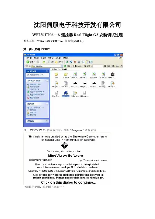
沈阳伺服电子科技开发有限公司WFLY-FT06－A遥控器Real Flight G3安装调试过程准备工作：WFL Y-TDF-FT06－A、加密狗(USB口)第一步：安装PPJOY打开PPJOY V0.83 的安装目录，点击“Setup.exe”进行安装出现提示界面，在界面上点击一下点击“Next”点击“Next”如果不换安装目录的话，点击“Next”点击“Next”点击“Next”等待安装安成提示硬件驱动安装，点击“仍然继续（Ｃ）”同上操作，点击“仍然继续（Ｃ）”安装完成后一弹出的已安装程序组提示的界面点击“Close”完成第二步：设置虚拟游戏端口在安装后弹出的界面中（或者是“开始”－“程序”－“Parallel Port Joystick”）中，点击“Configure Joysticks”点击“Add”按钮在Parallel Port 项选择“Virtual Joysticks”，再点击“Add”按钮选择第一项“是，仅这一次（Ｙ）”，再点“下一步”选择“自动安装软件（推荐）（Ｉ）”项，再点“下一步”点击“仍然继续（Ｃ）”按钮出现驱动安装过程点击“完成”按钮系统会自动提示找到Game Controller，并要求安装驱动，此过程会自动完成点击“完成”按钮“开始”－“程序”－“Parallel Port Joystick”）中，点击“Configure Joysticks”选择刚增加的那一项，并点击“Mapping…”选择第一项，如图，再点“ＯＫ”按钮选Modify the mapping for this controller选项，在点击“下一步”天地飞FT06-A的设置通道如上，一定要设置5个通道，否则遥控器1制式2号通道升降舵无反应。

注意圈红处设置。

点击“下一步”对应Slider的要设置为Analog 4，否则遥控器1制式2号通道升降舵无反应。

注意圈红处设置。

点击“下一步”点击“下一步”点击“完成”点击“Ｄｏｎｅ”按钮完成设置第三步：安装ＰＰＪｏｙ音频插件点击“PlusSetup.msi”安装文件出现提示，点击“下一步”如果不改变安装目录的话，可直接点击“下一步”再点击“下一步”等待安装完成点击“关闭”以完成安装第四步：将破解文件(plusSetup破解.exe)复制到安装目录PPJOY插件调试过程：1．将配套加密狗连接到发射机和电脑（发射机需要发射电池，去掉晶体，打开发射机电源。

FLOW3DHydraulicsTutorial教程FLOW3D是一个用于模拟流体动力学的计算流体力学（CFD）软件。

它使用基于有限体积方法的算法来解决包括流体流动、传热和可扩散性等问题。

FLOW3D在水力学领域广泛应用，包括水坝和堤坝设计、河流和水域模拟以及废水处理等。

在本教程中，我们将介绍如何使用FLOW3D进行水力学模拟。

首先，我们需要准备模型的几何图形和边界条件。

在FLOW3D中，我们可以使用软件自带的几何建模工具或导入现有的CAD文件。

一旦几何模型准备好，我们需要定义流体的初始条件和边界条件。

例如，我们可以指定流体的密度、粘度和初始速度等参数。

边界条件可以包括入口和出口速度、压力和液面高度等。

接下来，我们需要选择合适的数值方法和求解器来求解模型。

FLOW3D提供了多种数值方法和求解器选项，可以根据需要进行选择。

一般来说，使用隐式差分方法和迭代求解器可以获得更准确的结果。

完成模型设置后，我们可以开始运行模拟。

FLOW3D会基于指定的初始条件和边界条件求解流体流动方程，并生成包括速度、压力和液面高度等信息的结果文件。

完成模拟后，我们可以使用FLOW3D内置的后处理工具来分析和可视化结果。

例如，我们可以绘制液面高度随时间变化的图表，或者生成流速和压力分布等图像。

除了基本的水力学模拟，FLOW3D还提供了其他功能，如多相流模拟、热传导模拟和湍流模拟等。

通过使用这些功能，我们可以更全面地研究水力学问题，例如流体与固体相互作用的影响、热传导对流体特性的影响等。

总而言之，FLOW3D是一个功能强大的水力学模拟软件，可以帮助工程师和研究人员解决各种流体动力学问题。

通过使用FLOW3D，我们可以更好地理解和优化水力系统的设计和运行，从而提高水力系统的效率和安全性。

开始对NT用户:从Windows NT Workstation菜单栏:选择‘Start’‘Programs’‘Vega’‘LynX’你将在屏幕上看到lynx系统界面。

在屏幕左侧一个图标按钮上点击可关闭当前显示的面板同时激活与所点图标相关联的面板，并随机打开。

缺省状态下在必要的情况说明下预览以下应用程序:system,channel,window,environment,graphic state,observer和a motion model。

图标滚动列主面板系统设置Goal:取消不用的模块在文件下拉菜单下选择Active Modules。

在这个对话框中你可以选择以下几项：Large Area DBM,Light Lobes, Symbology,Clip-Mapped Objects,和SensorVision。

通过你的选择，然后点击‘OK’，激活或者取消附加模块当你完成后选择点击‘OK'。

创建一个Vega对象物对象物是许多几何体的一个集合。

在一个场景中涉及许多对象物，合起来代表一种可见的情景景物。

更多细节请参看Vega LynX User's Guide Chapter5。

Goal:创建一个静态的Vega对象物在图标滚动栏中点击object按钮。

从Objects下拉菜单中选择‘New'。

将会出现一个‘New Object'的对话框。

在文件编辑栏中键入‘terrain’来命名object实例。

注意:用户确定所命名的名字，可以选择熟悉的名字，以便快速确认使用的几何文件。

点击‘OK'。

此时，lynx界面如下图：文件浏览器控制按钮使用文件浏览器(?)结合你要使用的对象物场合选择你要插入的几何模型文件。

你将在如下路径<Installation Drivefor Vega>\Vega\Sample\Data\Vega\找到Open Flight文件格式的例子。

Ⳃ㄀ϔゴ ⿟ⱘ ゟ1.1 ⿟ (1)1.2 ⬏䴶㓪䕥 (2)㄀Ѡゴ⬏䴶Ӵ䕧2.1 Ӵ䕧䆒㕂 (4)2.2 ⬏䴶Ӵ䕧 (6)2.3 ῵ ԰ (9)㄀ϝゴ ⫼ Parts ҟ㒡3.1 ԡ (10)3.2 (13)3.3 㛑 (15)3.4 㡆♃ (17)3.5 ⼎ (18)3.6 䬂Ⲭ䕧 ⼎ (20)㄀ ゴ GP ㋏㒳 Ϣ L S4.1 GP ㋏㒳 (26)4.2 L S ㅔҟ (27)⊼1˖㋏㒳 ⱘ㣗 (28)⊼2˖⡍⅞㒻⬉ (33)㄀ϔゴ ⿟ⱘ ゟ1.1 ⿟㗙Ң[ ] -> [⿟ ] -> [Pro-face] -> [ProPB3C-Package] 䗝 [Project Manager]ˈ ⿟ㅵ⧚ ⼎ ⿟ㅵ⧚ ⬏䴶⿟ㅵ⧚ Ё⚍ [New] 䪂ˈ ⦄ҹϟ 䆱Ḛ˖Descriptior˖ ⿟ 䗄GP Type˖䗝 Փ⫼ⱘGP㋏Serial I/F Switch˖䗝 Փ⫼ COM1COM2 䖲 PLCDevice/PL C Type˖䗝 PLC䗴 䗮 䆂Extend SIO Type˖䗝 І 㽕䖲ⱘ䆒 ˄ ҹ ⷕ䯙䇏 ǃ⏽ ǃ㞾 Н䗮䆃 䆂ㄝ˅䆒㕂 ҹ ⚍ [OK] 䗝 ⬏䴶㓪䕥 DŽ䕃ӊ 䮼 䆁1.2 ⬏䴶㓪䕥㓪䕥⬏䴶に䕃ӊ 䮼 䆁Ϟ 㓪䕥⬏䴶に Ё⚍ ⬏䴶䪂ˈ✊ に Ё䗝 [Base Screen]⬏䴶ˈ⚍ [OK] 䪂ˈ䖯 ⱘ㓪䕥⬏䴶DŽⱘ㓪䕥⬏䴶ˈ ϟ ⼎˖䕃ӊ 䮼 䆁㄀Ѡゴ⬏䴶Ӵ䕧ゴҟ㒡⬏䴶 Ӵ䕧 乏䖯㸠ⱘ 䆒㕂DŽ2.1Ӵ䕧䆒㕂Ӵ䕧にℸ⬏䴶Ё⚍ [Transfer Settings] ˈ [Setup] 㦰 Ё䗝 [Transfer Settings] 䗝乍ˈ ⦄ҹϟ⬏䴶DŽ䕃ӊ 䮼 䆁ƹ䗮䆃ッ (Communication Port)[COM]˖Փ⫼Ӵ䕧⬉㓚˄GPW-CB02/GPW-CB03˅ϟ䕑⿟ ˈ䗝 ⱘІ㸠 ҹ Ӵ䕧䗳⥛˄⊶⡍⥛˅DŽGP2000 ㋏ ⱘ㾺 ˈӴ䕧䗳⥛ ҹ䖒 115.2KDŽ[Ethernet]˖䕧 IP ッ DŽ[Ethernet:Auto Acquist]˖㞾 ㋶䖲 㔥㒰ЁⱘGPⱘIP DŽƹӴ䕧 (Transfer Method)[Send All Screens]˖ ϔϾ ⿟ ӊЁⱘ ⬏䴶 䛑Ӵ䕧 㾺 DŽ[Automatically Send Changed Screens]˖㞾 Ӵ䕧 ⿟ ӊЁ 䖛ⱘ⬏䴶DŽ䗝 њ䖭⾡Ӵ䕧 ˈ䙷М GP 䕃ӊЁ 㹿 䰸ⱘ⬏䴶ˈ Ӵ䕧 ↩ ϡӮ㞾 䰸㾺 ϞⱘⳌ ⬏䴶DŽ 㽕 ⬏䴶ˈ䖬 㽕䗝 ĀSend All ScreenāDŽԚ ˈ Փ䗝 ĀSend All Screenāгϡ㛑 䰸 CF Ϟⱘ DŽ[Send User Selected Screens]˖ ḍ 䳔㽕ˈӴ䕧 ⱘ⬏䴶DŽ˄ 䜡 Ctrl 䬂 Shift 䬂䗝 ˅⊼ ˖ ḷ ǃ䆄 ䷇ ⊩䗝 ⱘDŽƹ䆒㕂 (Setup)[Automatic Setup]˖ḍ GP ⱘ⢊ ˈ 䳔㽕ˈ 㸠䖭Ͼ䆒㕂 ԰DŽϔ㠀䛑䗝 [Automatic Setup] ῵ DŽ[Force System Setup]˖ϡㅵ GP ⱘ⢊ ԩˈ↣⃵ ⬏䴶Ӵ䕧 ˈ䛑㽕 㸠ϔ⃵㋏㒳䆒㕂DŽ[Do Not Perform Setup]˖⬏䴶 Ӵ䕧 ˈϡ 㸠䆒㕂DŽƹ䆒㕂 CFG ӊ(Setup CFG File)䖭Ͼ ӊ 䆒㕂 ⱘˈ䗮 ϡ䳔㽕⫼ DŽ䕃ӊ 䮼 䆁ƹϟ䕑⬏䴶 ӊ (Send)[Send] 䪂ˈ⿟ ҢPCϟ䕑 GPDŽƹϞӴ⬏䴶 ӊ (R eceive)[Receive] 䪂ˈ⿟ ҢGPϞӴ PCDŽƹ῵ (Simulation)䆒㕂 䳔㽕䖯㸠῵⊼ ˖ 䕃ӊⱘ῵ PC ῵ PL Cˈ ҹ䗮䖛䕃ӊ ϡ䖲 PL C ⱘ ϟ䖯㸠῵ ⼎DŽ2.2 ⬏䴶Ӵ䕧GP ⬏䴶 3⾡Ӵ䕧 ˖⬉㓚Ӵ䕧ǃCF Ӵ䕧ǃ㔥㒰Ӵ䕧DŽ2.2.1 䗮䖛⬉㓚Ӵ䕧䗝 [COM] ˈ䆒㕂Ӵ䕧䗳⥛DŽ䖯㸠Ӵ䕧 ⬉㛥 GP П䯈䖲 ϔḍ⬏䴶Ӵ䕧⬉㓚˄GPW-CB02 GPW-CB03˅ ˈӴ䕧䆒㕂 ϟ ⼎DŽӴ䕧⬉㓚ϔッ GP ⱘTOOL ˈ ϔッ ⬉㛥ⱘCOM(CB02) USB(CB03) DŽ⊼ ˖⫼ CB03 Ӵ䕧 ˈ㽕 ⬉㛥Ϟ 㺙偅 ⿟ DŽ2.2.2 䗮䖛㔥㒰Ӵ䕧䗝 [Ethernet]䆒㕂Ⳃ GP ⱘ IP ˈPort˄ッ ˅˖8000˄ ˅䗝 [Ethernet˖Auto Acquist]Ӵ䕧 ˈ㋏㒳䗮䖛㞾 Ẕ ˈ ⼎ 㔥㒰Ё 䖲 ⱘGP ⱘIP DŽ䗝 GP ⱘIP ˈ 䖯㸠⬏䴶Ӵ䕧DŽ⊼ ˖ℸ⾡Ӵ䕧 䗖⫼ѢGP2000 ㋏ ˄GP2000㋏ Ёⱘ 01 䰸 ˅ƹ䆒㕂Ӵ䕧 ⷕ䆒㕂Ӵ䕧 ⷕ ҹ䰤 ϞӴǃϟ䕑ⱘ 䰤䆒㕂䖛⿟ ϟ ⼎䕃ӊ 䮼 䆁2.3῵ ԰Փ⫼⬏䴶Ӵ䕧⬉㓚 㗙㔥㒓 GP Ϣ⬉㛥䖲 䍋 DŽ✊ Ӵ䕧䆒㕂Ё䗝 [Simulation]䞡 Ӵ䕧⬏䴶 ˈ ⿟ㅵ⧚ ⬏䴶Ёˈ⚍ 䖯㸠῵ ԰DŽ [Start] 䪂 ῵ ˗ [Cancel] 䪂㒜ℶ῵ DŽ㄀ϝゴ ⫼Parts ҟ㒡ゴҟ㒡 ⬏䴶 ԰ 㒣 Փ⫼ⱘϔѯ Parts ⱘ԰⫼ ㅔ 䆒㕂DŽ3.1 ԡ ˄Bit Switch˅ԡ ϔ⾡㾺 ˈ⫼Ѣ ϔϾԡ ⱘ ON/OFF ⢊ DŽ⊼ ˖ GP ≵ 䖲 PL C ˈGP Ϟϡ ⼎ ⲥ㾚 㛑ⱘԡ ˈ GP Ϣ PL C 䖲 ℷ ˈ ⼎䆹 DŽƹϔ㠀䆒㕂 (General Settings)[ ԰ԡ (Operation Bit Address)]䕧 ⱘԡ DŽ[ⲥ ԡ (Monitor Bit Address)][ⲥ (Monitor)] 䗝Ḛ㹿䗝Ё ˈ ⱘ ⼎⢊ 㛑 ✻ⲥ ԡ ⱘPLC ԡⱘ ON/OFF ⢊ 㗠 DŽ[ 㛑(Function)]ԡ ⦄ⱘ 㛑 ϟ ⾡ˈ䇋ҢЁ䗝 ϔ⾡DŽ㕂ԡ(Bit Set)˖ 㹿 ϟ ˈPLC Ⳍ ⱘԡ㹿㕂Ў ONDŽ˄⢊ ˅ԡ(Bit Reset)˖ 㹿 ϟ ˈPLC Ⳍ ⱘԡ㹿㕂Ў OFFDŽ˄⢊ ˅ⶀ (Momentary)˖ 㹿 ϟ ˈPLC Ⳍ ⱘԡ㹿㕂Ў ONˈˈPLC Ⳍ ⱘԡ䕀Ў OFFDŽԡ 䕀(Bit Invert)˖↣ ϔ⃵ ˈ PL C Ⳍ ԡⱘ⢊ ⫳ DŽ˄ON→OFF OFF→ON˅ƹ 㾖/买㡆 (Shape/Color)䗝 ԡ ⱘ䖍Ḛ [ON/OFF] ⱘ [Fg ( )/ Bg (㚠 )] 买㡆DŽ⊼ ˖ ѯԡ 䚼ӊⱘ䖍Ḛ买㡆 /㚠 买㡆ϡ㛑 DŽϟ[Browser] ϟ䴶に ˈ䗝 䚼ӊ 㾖DŽƹ ㅒ (Label)䖭䞠 ҹḍ ԡ [ON/OFF] ⢊ ⱘϡ 䕧 ϡ ⱘ ㅒDŽƹ 㛑 (Extend)3.2 ˄Word Switch ˅⫼Ѣ ⱘ ˄ ˅ⱘ ⱘ㾺 DŽƹ ϔ㠀䆒㕂 (GeneralSettings)[ (Constant)]䕧 ԰ DŽ Ў 䖯 ˈ 㣗 ˖-32768̚32767DŽ[ 㛑(Function)]ҹϟ 㛑˖䆒㕂 (Word Set)˖ ϟ ˈ 㹿 ⱘ ˄ ˅ЁDŽ / (Add/Sub)˖ ϟ ˈ ˄ ˅ⱘ Ⳍ ˈ㒧 䆹 ˄ ˅DŽ Ў䋳 ˈ 㸠⊩䖤ㅫDŽԡ ԰˄ ˅(Digit ADD)˖ ϟ ˈ ˄ ˅ ⱘ ԡ1ˈԚϡ䖯ԡDŽ ҹ Bin BCDDŽ˄Ḑ 䗝 BCD ˈ Ў9ˈ 1 Ў0˗Ḑ 䗝 Ѡ䖯 ˈ ЎFˈ 1 Ў0˅DŽԡ ԰˄ ˅(Digit SUB)˖ ԡ 㸠 1 ԰ˈ 䖯ԡ ϞDŽƹ ㅒ (Label)䗝 [Direct]ˈ䕧 ϞⱘˈGP2000 ㋏ W indowsԧDŽ䗝 [Image Font]䗝乍ˈ✊ ⚍[Select Font]ˈ ҹՓ⫼ 䅵ㅫⱘ Windows ԧDŽҹ䗝 ԧⱘ ǃ 唤 ǃḋ ҹ 买㡆DŽƹ 㛑 (Extend)3.3 㛑 ˄Function Switch ˅㛑 㸠 㛑ⱘ㾺 DŽƹ ϔ㠀䆒㕂 (General Settings)[ ⫼ 㛑 (Function)]Previous Screen ˖ ϟ ˈ䏇䕀 ϔ ⬏䴶DŽGo To Screen ˖ ϟ ˈ䏇䕀 ⬏䴶DŽ䗝 ⱘ Ḑ ˄BCDѠ䖯 ˅ Ϣ GP 䆒㕂ϔ㟈DŽR eset GP ˖ ϟ ˈGP 㹿 ԡϔ⃵DŽƹ ㅒ (Label)䗝 [Direct]ˈ ✊ T ext ḚЁ䕧 䪂Ϟ ⼎ⱘ DŽ䖬 ҹ䗝 Փ⫼ Windows ԧˈ Ϩ䆒㕂 ԧⱘ ǃḋ 买㡆DŽƹ 䆒㕂 (Extend)䕃ӊ 䮼 䆁3.4 㡆♃˄Lamp ˅⼎♃Ⳉ ⲥ㾚 PL C ԡⱘ ON/OFF ⢊ DŽƹ ϔ㠀䆒㕂 (General Settings)[ԡ (Bit address)]䆒 㡆♃ 㽕ⲥ㾚ⱘԡ DŽƹ 㾖买㡆 (Shape/Color)⊼ ˖ ѯ♃ 䚼ӊⱘ Ḛ 买㡆 /㚠 买㡆ϡ㛑 DŽ䕃ӊ 䮼 䆁 ƹ ㅒ䆒 (Label)䕧 㡆♃䚼ӊⱘ ㅒˈг[ON/OFF] ϸ⾡⢊ ҹՓ⫼DŽ䗝 [Image Font]ˈ✊ ⚍[Select Font]ˈ ҹՓ⫼Windows ԧDŽ3.5 ⼎˄Numeric Display˅ҹ㒱 ⼎ PL C ˄ ˅ⱘ DŽƹϔ㠀䆒㕂 (General Setting)[ ˄Word Address˅]䕧 㹿 ⼎ ⱘ ˄˅DŽ[⌣㾜˄Browser˅]䗝 䚼ӊⱘ 㾖DŽ䕃ӊ 䮼 䆁 ƹ ⼎Ḑ ˄Data Display Format˅ℸ 䗝 ⼎Ḑ ǃヺ ǃ䭓 DŽḐ ˖ 䖯 ǃ 䖯 ǃBCDǃ 䖯 DŽ䭓 ˖16 ԡǃ32 ԡDŽ⼎ԡ (No.of Display Digits)˖䕧 ⼎ⱘ ԡ DŽ⚍ԡ㕂 (Decimal Places)˖䕧 ԡ DŽ⼎ (Display Style)˖唤䖬 唤ˈҹ ⚍ ⱘ ԡ䳊 㽕 ⼎DŽShift Right/ Shift Left˖ / 唤DŽZero Suppress˖ ⼎ϡ 㽕ⱘ0ˈ՟ ˖䗝 ⼎ 45ˈϡ䗝 ⼎0045DŽZero Display˖ Ў 0 ˈ䗝 ˈ ⼎[0]DŽϡ䗝 ˈϡ ⼎0DŽ7 Segment Display˖ ⼎Ў 7 ↉ ⷕㅵⱘ DŽƹ 㾖/买㡆 (Shape/Color)[⌣㾜˄Browser˅]䗝 䚼ӊⱘ 㾖DŽ䗝 ⼎䚼ӊⱘ䖍Ḛ ⼎ⱘ买㡆DŽƹ 䄺䆒㕂 (Alarm settings)[ 䄺㉏ (Alarm Type)]䗝 [Alarm Display]ˈ ⫳ 䄺 ҹ ԧ买㡆 䖍Ḛ买㡆ˈ 䄺㣗 DŽ 䄺㣗 ϸ⾡䆒㕂 ⊩˖[Direct]˖Ⳉ 䄺㣗 ˈ ⱘDŽ[ 䄺㣗 (Alarm R ange)][Direct] ῵ ϟ䆒㕂 䄺㣗 DŽ[Indirect] ῵ ϟ ⼎ 䄺㣗 ⱘ䆒㕂 DŽ[ 䄺买㡆(Alarm Color)]䆒㕂 ⫳ 䄺 ˈ ⼎ⱘ 㾖买㡆 ヺ买㡆DŽ3.6䬂Ⲭ䕧 ⼎˄Keypad Input Display˅⫼Ѣ ⼎䬂Ⲭ䕧 ˈ䬂Ⲭ䕧 ⱘ ⱘDŽƹϔ㠀䆒㕂 (General Settings)[ (Word Address)]⫼Ѣ 䬂Ⲭ䕧 ⱘ DŽ[㾺 (Start)][Start] 䗝 [Touch] ˈϡ䳔㽕䆒㕂㾺 ԡˈ 䖤㸠 Ⳉ 㾺 ˈ䬂Ⲭ 䕧 㹿▔⌏ˈϨ 䖍 ⦄ϔϾ䬂ⲬDŽ[Start] 䗝 [Bit] ˈ㽕䆒㕂ϔϾ[㾺 ԡ (Trigger Bit Address)]ˈ 䆹ԡЎ ON ⢊ ˈ䬂Ⲭ 䕧 㹿▔⌏ˈ䬂Ⲭ䕧 ⱘ 䆹 ⼎に⼎ˈ ϟ䬂Ⲭⱘ [ENT] 䬂 ˈ䕧 㹿 ⱘ DŽƹ ⼎Ḑ ˄Display Format˅ϝ⾡Ḑ ˖AbsoluteǃRelativeǃChar.StringDŽЏ㽕ҟ㒡㒱 ⼎Ḑ DŽ[㒱 (Absolute)]˖ ⼎ ⼎ⱘ 䕧 ⱘ 䰙 DŽ[Indirect]˖⫼䯈 䇏 ˈ䇏 ⱘ䅵ㅫ ⊩ [ ˄Base Address˅] Ϟ Ё ⱘ DŽ[Addresses]˖ DŽ[Device type & Address]˖ [General Settings] Ё䆒㕂ⱘ ⱘ ⸔Ϟ 1DŽ[Display & Write Data Format]˖䆒㕂 ⼎ 䇏 ⱘḐ DŽ䖬 ҹ䆒㕂 ⼎ⱘ䭓 ǃ㽕∖ ⼎ⱘ ԡ ҹ ⼎ ヺⱘ ㄝDŽϸ⾡ ⼎Ḑ ⱘㅔ 䆒㕂˖[Ⳍ (Relative)]˖䳔㽕䆒㕂䕧 ⱘ㣗 ⼎㣗 ˈ ⼎ ⼎ⱘ 䕧 ⱘ 䰙 㒣䖛䕀 ⱘ DŽ[ ヺІ (Char.String)]˖䳔㽕䆒㕂 ⼎ ヺІⱘ䭓ⷁDŽƹ 㾖/买㡆˄Shape/Color˅[⌣㾜(Browser)]⚍ [Browser]ˈ ⼎ 䗝 ⱘ 㾖ˈ ҹ䗝 ⱘDŽ[买㡆㉏ (Color Type)]ҹ⫼ [direct] [indirect] 䆒㕂 ⼎ⱘ买㡆DŽ[direct]˖Ⳉ 䆒㕂买㡆DŽ[indirect]˖䆹䆒㕂 㡆 ⱘҷⷕ 䆒㕂 Ā+1āⱘ ЁDŽ ⼎Ḑ Ў [absolute] 㛑䆒㕂Ў䯈 ῵ DŽ[䗝 䯈 (Select Indirect Address Area)][Absolute] Ḑ ⱘ [Indirect] 䗝乍ϟ 㛑Փ⫼DŽ ϟϔϾⱘ䖲㓁 Ё ҹ䆒㕂买㡆ҷⷕDŽ[䖍Ḛ买㡆/ 买㡆/ 㡆(Border Color/Text color/Plate color)]䚼ӊⱘ䖍Ḛ买㡆ǃ ⼎ⱘ ԧ买㡆 㚠 买㡆DŽƹ 䄺䆒㕂 (Alarm Settings)[ 䄺㉏ (Alarm Type)]䗝 [Alarm Display]ˈ ⫳ 䄺 ҹ ԧ买㡆 䖍Ḛ买㡆DŽϝ⾡ 买㡆ⱘ ⊩˖Direct˖ ҹ 䄺㣗 ˈ Ϩ ⱘDŽIndirect˖ 䄺㣗 䆒㕂 ⿏ 䞠ⱘˈ ⱘDŽColor Change˖ ԡЎ ON ˈ䆒㕂买㡆 DŽ[ 䄺㣗 (Alarm Range)][Direct] ῵ ϟ䆒㕂 䄺㣗 DŽ[Indirect] ῵ ϟ ⼎ 䄺㣗 ⱘ䆒㕂 DŽ[ 䄺买㡆(Alarm Color)]䆒㕂䍙 䄺㣗 䕧 ⼎ⱘ Fg ( 㡆) Bg (㚠 㡆)DŽ[䗝 䯈 (Select Indirect Address Area)][Absolute] Ḑ ⱘ [Indirect] 䗝乍ϟ 㛑Փ⫼DŽ ϟϔϾⱘ䖲㓁 Ё ҹ䆒㕂买㡆ҷⷕDŽ䕃ӊ 䮼 䆁 ㄀ ゴ GP ㋏㒳 ϢLS4.1 GP ㋏㒳GP Ϣ PL C ⱘ䗮䆃ЁˈGP ⬏䴶 ⼎ 䳔ⱘ ⬅ GP 㞾 䇋∖ ˈ㾺 䬂ⱘ ԰䕧 ⬅ GP 㞾 Ӵ䕧 PL CDŽ PL C Ϟˈϡ䳔㽕Ў⬏䴶 ⼎ǃ ԰㓪 ϧ⫼ⱘ⿟ DŽGP ㋏㒳 ⱘ䍋 ԡ㕂㋏㒳 GP Ё ⱘϔ䚼 ˈ PL C Ё䳔㽕 䕳 ⱘ㋏㒳 ˈ䖯㸠 GP 䖤㸠Ё ⾡ ⱘⳌѦѸ DŽҢ GP ⱘ[INITIALIZE/STARTING ADDRESS OF SYSTEM DATA AREA]Ё䆒㕂GP Ϣ PL C П䯈ⱘ㋏㒳䗮䆃 DŽƹḍ PL C ㉏ ˈ ѯ ˄ 䚼 ˅ ҹ䆒㕂Ў㋏㒳 DŽ 䖭ѯ Ёˈ 㹿 PL C Ҫ⿟ Փ⫼ⱘ ˈ ⫼Ѣ㋏㒳 DŽ䕃ӊ 䮼 䆁4.2 LS ㅔҟGP ⱘ L S ˈ ⫼Ѣ GP ԰ⱘ DŽLS ⱘ ϟ˖⊼˖ GP2000 ㋏ Ё ҹՓ⫼ L S8191ˈ GP77Rҹ ⱘ㋏ Ё ҹՓ⫼ LS4095DŽ㋏㒳 ˖䖭 GP ԰Ё 乏ⱘ⬏䴶 䫭 ⱘ DŽ䇏 ˖ ⬏䴶ⱘ ⫼ ǃ䍟 ⼎ ˈ 䆒㕂 256 DŽ⫼ ˖䖭ѯ ҙ㛑 GP 䚼Փ⫼ˈϡ㛑 PL C Ё 䜡DŽ䖭Ͼ ⫼Ѣ䙷ѯҙ GP 䚼 ⧚ⱘ䚼ӊ Tagˈϡ㛑⬅ PL C DŽ⡍⅞㒻⬉ ˖䖭Ͼ GP 䗮 䯈 ⾡⢊ DŽƹ ԩ LS䕃ӊ 䮼 䆁 ⊼1˖㋏㒳 ⱘ㣗ϟ㸼㾷䞞Ⳉ 䗮䆃 ㋏㒳 ↣Ͼ ⱘ DŽ乍Ⳃ ԡ㾷䞞GP PLC 1 +0 ⼎⬏䴶1-8999˄ ⫼BCD ˈЎ1-9999˅2 +1䫭⢊ 0ˈ1 ⫼↣Ͼԡⱘ ˈ䫭⢊ DŽ ⫳ 䫭ˈԡЎONDŽON⢊ϔⳈ GP ⬉ 䕀ЎOFFLINE DŽ2 ㋏㒳ROM/RAM3 偠4 SIO5 SIO6 SIO䍙䖤㸠7ˈ8 ⫼9 䳔㽕10 䩳 䫭11 PLCⱘSIO 䫭12-15 ⫼3+2 Ā āˈϸԡBCD ӑⱘ ϸԡ+3 Ā āˈϸԡBCD 01-12˄ ӑ˅+4 Ā āˈϸԡBCD 01-31˄ ˅+5Ā 䯈āˈ ԡBCD˄00-23˅ˈ 䩳˄00-59˅4 +6 ⢊ *50ˈ1 ⬭*52 ℷ *1 *53 ϔϾ䆒㕂 *2 *54-6 ⬭*57 PLC⣀ *3 *58 K-tag䕧 䫭*4 *59-15 ⬭*55 +7 ⬭PLC GP 6 +8 ⼎⬏䴶1-8999˄ ⫼BCD ˈЎ1-9999˅7 +9 ⬏䴶 ⼎ON/OFF*130˄h˅˖ ⼎ONFFFF˄h˅˖ ⼎ 䯁8+10䩳Ā ā䆒㕂 ˄+˅BCDϸԡӑⱘԢϸԡ˄15#ԡ䩳 *6 +11䩳Ā ā䆒㕂 ˈBCDϸԡ01-12˄ ӑ˅䩳Ā ā䆒㕂 ˈ䕃ӊ 䮼 䆁+13 䩳Ā 䯈ā䆒㕂 ˈBCD ԡ˄00-23˅ˈ 䩳˄00-59˅PLC GP 乍Ⳃ ԡ㾷䞞9 +14䫭⢊ 0㚠 ♃OFF*7*121 㳖号 ON23 ⬭4㳖号 *80˖ 䆌˗1˖⽕ℶ5䕙 䕧 *80˖ 䆌˗1˖⽕ℶ6 ⬭7PLC⣀ *90˖⽕ℶ˗1˖ 䆌8VGA ⼎*100˖⽕ℶ˗1˖ 䆌9ˈ10 ⬭11⹀ 䋱䕧 *140˖ 䆌˗1˖⽕ℶ12-15 ⬭A +15 ⬭䆒㕂Ў0B +16 に *11⼎ˈ0˖OFF˗1˖ON1に 㽚Ⲫⱘ⃵ˈ0˖ ˗1˖ϡ2-15 ⬭C +17 に ⊼ *11⫼䯈 䆒㕂䗝 に ⊼˄BIN/BCD˅D+18に ⼎ԡ㕂˄X ˅⫼䯈 䆒㕂䗝 に ⼎˄BIN/BCD˅+19に ⼎ԡ㕂˄Y ˅⊼䞞˖*1 Ёˈ䖭Ͼԡ Ӯ ONDŽ ℸԡЎON ˈ䖯 GP ⱘOFFLINE ῵ ˈ⾏ 䕧 DŽ*2 ↣⃵Փ⫼K-Tag Parts ⱘKeypad Input Display ˈ䖭Ͼԡ Ӯ ⳌDŽ䕃ӊ 䮼 䆁*3 Փ⫼Multi-Link ῵ ˈ PLC ⫼Ёˈ䖭Ͼԡ Ӯ ONDŽ*4 Փ⫼K-Tag ⱘAlarm 㛑 ˈ 䍙 䆒㕂ⱘ㣗 ˈ䖭Ͼԡ Ӯ ONDŽ Пˈ 䍙 䆒㕂ⱘ㣗 ˈ䖭Ͼԡ Ӯ OFFDŽ*5 ⲥ 䳔ⱘԡDŽ ⬭ⱘԡˈ⫼԰GP ⱘ㋏㒳 ㄝ ԰ˈON/OFF ⢊НDŽ*6 (ԡ 15)ˈ⬅ON→OFF OFF→ONˈ ⱘ 䯈 DŽ՟ ˖ 2002 10 16 9:57 PMⳂ +10 ⱘ Ў0000(BCD)ˈ ˈ ϟ˖ƽ +11ⱘ Ў0010(BCD)ƽ +12ⱘ Ў0016(BCD)ƽ +13ⱘ Ў2157(BCD)+10 ⱘ (ԡ 15) ⢊ ˈ DŽƽ +10 8002(BCD)ˈ DŽ*7 䰸њGP-477RˈGP-470 ҹ ˈ 䖭ϾԡЎON ˈ ⱘ㚠 䯁ˈ 䖭ϾԡЎOFF ˈ ⱘ㚠 DŽ+14 ԡ 0 ЎON ˈ ⱘ㚠 䯁ˈԚ ⱘ 䪂ձ✊ ҹ ԰ˈLCD ҡ✊ ⼎ˈՓ⫼ +9 ⱘON/OFF ԡ LCD ⳳⱘ ⼎DŽ*8 ԡ ON ⱘ ˈGP 䚼ⱘ㳖号 (Buzzer) Ѣ▔⌏⢊ DŽ*9 Փ⫼Multi Link ( n:1 )ˈPLC ⫼ ˈԡЎONDŽ*10 GP-570VM GP-870VMˈ Ͼ⬏䴶 ⦄ VGA ⼎῵ ˈ ϟ ⱘӏԩϔ⚍ˈ䖭Ͼԡ Ӯ OFFDŽ*11 Ѣに (Window) 㒚㡖ˈ 㗗 Tag 㗗 Ā2.26 U-Tag に ⼎ ā*12 䇋⹂䅸 ⱘ ⬭ԡ OFF ⢊ ˈг䆌䖭ѯ ⬭ԡ㹿GP ㋏㒳 Փ⫼DŽ ( +14), 䇋⫼ԡḐ DŽ ⫼ Ḑ ˈ 㛑 ԡⱘ⢊ .*13 䆒㕂 ⼎ⱘԡЎOFF П ˈ ϟ Ϟⱘӏϔ⚍ˈ ⼎ⱘԡЎONDŽ*14 㽕 Ⳃ ⼎ⱘ ˈ 䆒 +14ⱘԡ 11 ЎONDŽƽ ⍜ ˈ +14 ⱘԡ 11 ϡӮ㞾 OFFˈ ҹ Ẕ ⢊ ⱘ Ёԡ( +6 ⱘԡ 2)ЎOFF ⢊ ˈ +14 ⱘԡ 11䆒ЎOFFDŽƽ +14 ⱘԡ 11 ЎON ˈ ⊩䖯㸠 ⼎ⱘ DŽ䕃ӊ 䮼 䆁 ㋏㒳 ⫼ⱘLSLS0000: ⦄ ⼎ⱘ⬏䴶 ⷕ(1- 8999 ( Փ⫼BCD ⷕ 1 ~ 1999))LS0002: ⦄ - ˈ2 ԡBCD ⷕˈ ӑⱘ 2 ԡLS0003: ⦄ - ˈ2 ԡBCD ⷕˈ01-12( )LS0004: ⦄ - ˈ2 ԡBCD ⷕˈ01-31( )LS0005: ⦄ 䯈- ˈ4 ԡBCD ⷕˈ00-23( )ˈ00-59( )LS0006: ⲥ 䳔ⱘԡDŽ ⬭ⱘԡˈ⫼԰GP ⱘ㋏㒳 ㄝ ԰ˈON/OFF ⢊ НDŽLS000602: Ёˈ䖭Ͼԡ Ӯ ONDŽ ℸԡЎON ˈ䖯 GP ⱘOFFLINE ῵ ˈ⾏ 䕧 DŽLS000603: ↣⃵Փ⫼K-Tag Parts ⱘKeypad Input Display ˈ䖭Ͼԡ Ӯ ⳌDŽLS000607: Փ⫼Multi-Link ῵ ˈ PLC ⫼Ёˈ䖭Ͼԡ Ӯ ONDŽLS000608: Փ⫼K-Tag ⱘAlarm 㛑 ˈ 䍙 䆒㕂ⱘ㣗 ˈ䖭Ͼԡ Ӯ ONDŽ Пˈ 䍙 䆒㕂ⱘ㣗 ˈ䖭Ͼԡ Ӯ OFFDŽLS0008: ⼎ⱘ⬏䴶ˈ1- 8999 ( Փ⫼BCD ⷕ 1 ~ 1999)DŽLS0009: 䆒㕂 ⼎ⱘԡЎOFF П ˈ ϟ Ϟⱘӏϔ⚍ˈ ⼎ⱘԡЎONDŽLS0010: (ԡ 15)ˈ⬅ON OFF OFF ONˈ ⱘ 䯈 DŽ՟ ˖ 2002 10 16 9:57 PMⳂ +10 ⱘ Ў0000(BCD)DŽ ˈ ˈ ϟ˖+11 ⱘ Ў0010(BCD)+12 ⱘ Ў0016(BCD)+13 ⱘ Ў2157(BCD)+10 ⱘ (ԡ 15) ⢊ ˈ DŽ+10 2002(BCD)ˈ DŽLS0014: 䰸њGP-477RˈGP-470 ҹ ˈ 䖭ϾԡЎON ˈ ⱘ㚠 䯁ˈ 䖭ϾԡЎOFF ˈ ⱘ㚠 DŽ+14 ԡ 0 ЎON ˈ ⱘ㚠 䯁ˈԚ ⱘ 䪂ձ䕃ӊ 䮼 䆁✊ ҹ ԰ˈLCD ҡ✊ ⼎ˈՓ⫼ +9(LS0009) ⱘON/OFFԡ LCD ⳳⱘ ⼎DŽLS001404: ԡ ON ⱘ ˈGP 䚼ⱘ㳖号 (Buzzer) Ѣ▔⌏⢊ DŽLS001405: Փ⫼Multi Link ( n:1 )ˈ PLC ⫼ ˈԡЎONDŽLS001411: 㽕 Ⳃ ⼎ⱘ ˈ 䆒㕂 +14 ⱘԡ 11 ЎONDŽ ⍜ ˈ +14 ⱘԡ 11 ϡӮ㞾 OFFˈ ҹ Ẕ ⢊ⱘ Ёԡ( +6 ⱘԡ 2)ЎOFF ⢊ ˈ +14 ⱘԡ11 䆒㕂ЎOFFDŽ+14 ⱘԡ 11 ЎON ˈ ⊩䖯㸠 ⼎ⱘ DŽ(ҹϞЎ㋏㒳 ˈ х⫼DŽ 䳔Փ⫼ˈ䇋ձ✻㓧 ⡍ Փ⫼DŽ)䕃ӊ 䮼 䆁 ⊼2˖⡍⅞㒻⬉GPⱘ⡍⅞㒻⬉ ϟ˖LS2032 ⫼㒻⬉LS2033 ⬏䴶LS2034 ⬭L S2035 1⾦Ѡ䖯 䅵L S2036 Tag 䯈L S2037 SIO ⦃ 䯈L S2038 Tag 䅵LS2039 SIO 䫭ҷⷕLS2040 Ҹ⠠Ӵ䗦䗳 ҙ⫼Ѣn˖1( multi-link 䖲 ) LS2041 Ҹ⠠Ӵ䗦䗳L S2042 ̚LS2047⬭ƽ ⫼㒻⬉ ˄LS2032˅ƽ ⬏䴶 ˄LS2033˅ƽ ⬭˄LS2034˅⬭ ⱘ ϡ⹂ ⱘˈ䇋ϡ㽕Փ⫼䖭Ͼ DŽƽ 1 ⾦Ѡ䖯 䅵 ˄LS2035˅GP Ϟ⬉ ˈҹ 1 ⾦Ў ԡ䖯㸠䅵 DŽ Ѡ䖯 Ḑ DŽ䕃ӊ 䮼 䆁 ƽ Tag 䯈˄LS2036˅䆒㕂⬏䴶 ⼎ Tags 㢅䌍ⱘ 䯈DŽ ҹ ms Ў ԡ˄Ѡ䖯 ˅DŽ ⱘⳂ Tags ⧚ ˈ DŽ Ў0ˈ 䯈㊒ Ў±10msDŽƽSIO ⦃ 䯈˄LS2037˅Ң SIO Ⳃ ˄PLC 䚼㋏㒳 ˅ 䞣㺙㕂ǃ 㒧 ˈ1 Ͼ ⦃㢅䌍ⱘ 䯈DŽ ㋏㒳 Ⳃ 㺙㕂ⱘ ⧚ DŽ Ў0ˈҹ10ms Ў ԡDŽƽTag 䅵 ˄LS2038˅⼎⬏䴶Ϟ䆒㕂ⱘ Tags ⱘ ˈ 䅵 ˄Ѡ䖯 ԡ˅DŽƽSIO 䫭ҷⷕ˄LS2039˅⫳ SIO 䫭 ˈ ⫳ⱘ SIO 䫭ҷⷕ˄Ѡ䖯 ˅DŽƽ Ҹ⠠Ӵ䗦䗳 ˄LS2040˅Ҹ⠠ ˄PLC ⣀ 䗮 ˅ǃӴ䗦 n GP 㢅䌍ⱘ 䯈DŽ ЎѠ䖯 Ḑ ˄ҹ 10ms Ў ԡ˅DŽ ⬏䴶 ˈ ˈ Ў0DŽƽ Ҹ⠠Ӵ䗦䗳 ˄LS2041˅Ҹ⠠ ˄PLC ⣀ 䗮 ˅ǃӴ䗦 n GP 㢅䌍ⱘ 䯈DŽ ЎѠ䖯 Ḑ ˄ҹ 10ms Ў ԡ˅DŽ ⬏䴶 ˈ ˈ Ў0DŽ⊼ ˖ ⫳䭓 䯈ⱘ SIO 䫭ˈ 䗮 ⬉㓚 ℷ 䖲 ㄝˈ 㒜 㛑Ӯ 䍋㋏㒳 䫭DŽ ⫳㋏㒳 䫭ˈ䇋 GP 䖯㸠 ԡDŽ ⫼ 1 ⾦Ѡ䖯 䅵 Tag 䅵 ԰Ў W-Tag ⱘⲥ ԡ D 㛮 ⱘ㾺 ԡ ˈ 㛑Ӯ 䍋㋏㒳 䫭DŽ ⫳㋏㒳 䫭ˈ䇋 GP 䖯㸠 ԡDŽ。

魔兽争霸3人工智能脚本（AI JASS）初级教程JASS与其他的面向流程性质的编程语言很类似，所以在阅读以下内容之前，首先应该对流程性质的编程以及TRIGGER JASS有着一定的了解。

了解JASS语言并有一定的基础之后，你将很快的了解AI JASS。

AI JASS的概念最主要的是理解AI线程(Threads）的概念。

线程是什么？线程就象TRIGGER的一个循环判断语句，线程会不停的判断在线程程序列表内所缺少的元素，并去按照线程的指令排放顺序去完成它。

就象碗中的饭，有即吃，有即吃，有即吃，Loop......为什么不用TRIGGER去完成电脑的人工智能呢？由于使用TRIGGER相比之下可能会消耗大量的内存，所以，最好用AI线程来完成电脑的人工智能。

注意：线程只针对单个玩家进行运作。

AI的类型（Melee AI 和Campaign AI ）Melee AI 对战AI基本上完全可以利用WORLDEDITOR自带的AI编辑器(AI Edior)完成Campaign AI 战役AI（即“非对战AI”），可以详细了解以下内容即可制作一般常用的战役AI注：战役AI的用途十分广泛，完全可以利用其制作生存，3C，TD等类型的地图，并且免除了不停使用TRIGGER创造单位所带来的内存泄露。

线程(Threads)和触发器(Trigger)的区别AI脚本只能使用JASS函数库mon.j和mon.ai中的函数和量Trigger脚本只能使用mon.j和Blizzard.j中的函数和量线程只应用于AI脚本(AI JASS), 不能用于触发器脚本(Trigger Jass)触发器只应用用于触发器脚本(Trigger Jass),不能用于AI脚本(AI JASS)通常, 当AI脚本开始运行时只创建一个线程, 创建更多的线程可以用man.j的本地函数: native StartThread takes code func returns nothing运行方式的区别在于线程一旦开启即可自动运转，触发器必须调用或者借助事件的发生才可以运行。

⼤学英语综合教程3unit3Unit 3 Out of StepSection One Pre-reading Activities (1)I. Audiovisual Supplement (1)II. Cultural Background (1)Section Two Global Reading (2)I．Text Analysis (2)II. Structural Analysis (2)Section Three Detailed Reading (2)I.Text 1 (2)II. Questions (4)III. Words and Expressions (5)IV. Sentences (7)Section Four Consolidation Activities (7)I. Vocabulary (7)II. Grammar (10)III. Translation (13)IV. Exercises for Integrated Skills (14)V. Oral Activities (16)VI. Writing (17)Section Five Further Enhancement (19)I. Lead-in Questions for Text II (19)II. Text 2 (19)III. Memorable Quotes (22)Section One Pre-reading ActivitiesI. Audiovisual SupplementWatch the movie clip and answer the following questions.Script:Narrator: A German factory builds one of the world‘s most famous cars. The 911 is the icon of the sports car industry. It‘s the shape, it‘s the engine in the back, it‘s the feel it gives you, it‘s the emotion. The factory runs like a precision machine, building hundreds of engines a day. The product and our manufacturing process are one unit, and that‘s our secret of success. Automation, technology and skilled human labor combine to build 16 versions of the Porsche 911, including the 911 GT3.Questions:1. Where is the engine of the 911?In the back of the car.2. What‘s the secret of success of that factory?The product and their manufacturing process are one unit. Automation, technology and skilled human labor combine to build the Porsche 911. And the factory runs like a precision machine.II. Cultural Background1. Car culture has been a major niche lifestyle in America.2. In the 1950s, the post-war boom produced a generation of teenagers with enough income to buy their own cars. These cars became so much more than just modes of transportation. They were reflections of a lifestyle. The ability to tune and soup-up muscle cars gave average Joes the opportunity to show off their power, their speed and their style in a way that personified the car as character.3. Like Granny in Jan and Dean's 1964 song ―The Little Old Lady from Pasadena,‖ we can't keep our foot off the accelerator.4. We are crazy about our cars —and always have been. ―The American,‖William Faulkner lamented in 1948, ―really loves nothing but his automobile.‖5. We dream of cars as we dream of lovers.6. Americans have always cherished personal freedom and mobility, rugged individualism and masculine force.Section Two Global ReadingI．Text AnalysisMain Idea―Out of Step‖ is an exposition that presents the absurdity of the Americans‘ dependence on cars. The Americans, being so accustomed to using cars, have almost forgotten the existence of their legs. Wherever they go, they go in their cars. As a result, pedestrian facilities are neglected in city planning or rejected by the inhabitants.II. Structural AnalysisParagraph 1-6 The writer introduces his idea with an anecdote.Paragraphs 7-13 In this part, the author presents the fact that the Americans are habituated to using cars for everything. Paragraphs 14-20 In this part, the author explains that pedestrian facilities are neglected or discarded.Section Three Detailed ReadingI.Text 1Out of StepBill Bryson1After living in England for 20 years, my wife and I decided to move back to the United States. We wanted to live in a town small enough that we could walk to the business district, and settled on Hanover, N.H., a typical New England town —pleasant, sedate and compact. It has a broad central green surrounded by the venerable buildings of Dartmouth College, an old-fashioned Main Street and leafy residential neighborhoods.2It is, in short, an agreeable, easy place to go about one‘s business on foot, and yet as far as I can tell, virtually no one does.3Nearly every day, I walk to the post office or library or bookstore, and sometimes, if I am feeling particularly debonair, I stop at Rosey Jekes Caféfor a cappuccino. Occasionally, in the evenings, my wife and I stroll up to the Nugget Theatre for a movie or to Murphy‘s on the Green for a beer, I wouldn‘t dream of going to any of these places by car. People have gotten used to my eccentric behavior, but in the early days acquaintances would often pull up to the curb and ask if I wanted a ride.4―I‘m going your way,‖ they would insist when I politely declined. ―Really, it‘s no bother.‖5―Honestly, I enjoy walking.‖6―Well, if you‘re sure,‖ they would say and depart reluctantly, even guiltily, as if leaving the scene of an accident without giving their name.7In the United States we have become so habituated to using the car for everything that it doesn‘t occur to us to unfurl our legs and see what those lower limbs can do. We have reached an age where college students expect to drive between classes, where parents will drive three blocks to pick up their children from a friend‘s house, where the letter carrier takes his van up and down every driveway on a street.8We will go through the most extraordinary contortions to save ourselves from walking. Sometimes it‘s almost ludicrous. The other day I was waiting to bring home one of my children from a piano lesson when a car stopped outside a post office, and a man about my age popped out and dashed inside. He was in the post office for about three or four minutes, and then came out, got in the car and drove exactly 16 feet (I had nothing better to do, so I paced it off) to the general store6 next door.9And the thing is, this man looked really fit. I‘m sure he jogs extravagant distances and plays squash and does all kinds of healthful things, but I am just as sure that he drives to each of these undertakings.10An acquaintance of ours was complaining the other day about the difficulty of finding a place to park outside the local gymnasium. She goes there several times a week to walk on a treadmill. The gymnasium is, at most, a six-minute walk from her front door.11I asked her why she didn‘t walk to the gym and do six minutes less on the treadmill.12She looked at me as if I were tragically simple-minded and said, ―But I have a program for the treadmill. It records my distance and speed and calorie burn rate, and I can adjust it for degree of difficulty.‖13I confess it had not occurred to me how thoughtlessly deficient nature is in this regard.14According to a concerned and faintly horrified 1997 editorial in the Boston Globe, the United States spent less than one percent of its transportation budget on facilities for pedestrians. Actually, I‘m surprised it was that much. Go to almost any suburb developed in the last 30 years, and you will not find a sidewalk anywhere. Often you won‘t find a single pedestrian crossing.15I had this brought home to me one summer when we were driving across Maine and stopped for coffee in one of those endless zones of shopping malls, motels, gas stations and fast-food places. I noticed there was a bookstore across the street, so I decided to skip coffee and head over.16Although the bookshop was no more than 70 or 80 feet away, I discovered that there was no way to cross on foot without dodging over six lanes of swiftly moving traffic. In the end, I had to get in our car and drive across.17At the time, it seemed ridiculous and exasperating, but afterward I realized that I was possibly the only person ever to have entertained the notion of negotiating that intersection on foot.18The fact is, we not only don‘t walk anywhere anymore in this country, we won‘t walk anywhere, and woe to anyone who tries to make us, as the city of Laconia, N.H., discovered. In the early 1970s, Laconia spent millions on a comprehensive urban renewal project, which included building a pedestrian mall to make shopping more pleasant. Esthetically it was a triumph —urban planners came from all over to coo and take photos--but commercially it was a disaster. Forced to walk onewhole block from a parking garage, shoppers abandoned downtown Laconia for suburban malls.19In 1994 Laconia dug up its pretty paving blocks, took away the tubs of geraniums and decorative trees, and brought back the cars. Now people can park right in front of the stores again, and downtown Laconia thrives anew.20And if that isn‘t sad. I don‘t know what is.II. Questions1)What kind of town is it? (Paragraph 1)It is a small, pleasant and agreeable town. The inhabitants are friendly and willing to help.But although the town is compact, few people go about on foot.2)What is considered the author‘s ―eccentric behavior‖? (Paragraph 3)Instead of riding a car, the author walks around the city, doing his shopping, going to themovies or visiting the café or bar. To people who are used to going everywhere in a car, he is an eccentric.3)Why would drivers ―depart reluctantly, even guiltily‖when their offer was declined?(Paragraphs 3-6)With cars becoming the basic essentials of their life, people are so habituated to using the car for everything. The scene of somebody walking around seemed so unusual to them that they would naturally show their concern to him. When their offer to give him a ride was declined, they were sorry for not being able to help him out.4) Why did the author say ―Actually, I‘m surprised it was that much‖? (Paragraph 14)When the author found that the newly planned suburbs totally overlooked pedestrian needs, he assumed there was no budget for pedestrian facilities at all. So he says he was surprised to learn that there actually was less than one percent of budget on it. Here the author writes with a touch of irony.5) Why did Laconia change its downtown pedestrian mall to one with parking lots? (Paragraphs18-19)Although the pedestrian mall was well decorated, shoppers were unwilling to walk to the stores from a parking garage. As a result, it was a commercial failure. The government had to compromise with the public preference.Class ActivityGroup discussion: What does the title mean?With the use of this title, the writer seems to suggest1. people no longer walk in America;2. the few people who do walk seem to be old-fashioned and ―eccentric‖.III. Words and ExpressionsParagraphs 1-6sedate a. calm, serious and formale.g. She is a sedate old lady; she is caring but never talks much.The fight against a nuclear power station site has transformed a normally sedate town into a battlefield.v. make calm or sleepy, esp. with a druge.g. The patient was heavily sedated and resting quietly in bed.Derivation: sedately (ad.), sedation (n.), sedative (a., n.)eccentric a.(of people or behavior) unconventional and slightly strangee.g. The old gentleman, who lived alone all his life, was said to have some eccentric habits.n. a person of unconventional and slightly strange views or behaviore.g. The old gentleman enjoyed a colorful reputation as an engaging eccentric.curb n. (British English: kerb) a line of raised stones separating the footpath from the road v./ n. ( place) a control or limit on sth. undesirablee.g.Poor nutrition can curb a child‘s development both physically and mentally.There will be now curbs on drunk-driving from next month.Paragraphs 7-12habituate v. accustom by frequent repetition or prolonged exposuree.g. You must habituate yourself to reading aloud.By the end of the school term, the students had been habituated / accustomed / used to rising at five o‘clock.contortion n. a twisted position or movement that looks surprising or strangee.g. The spectators cannot but admire the contortions of the gymnasts.Derivation: contort v. cause sth. to twist out of its natural shape and looks strange or unttractive Comparison: distort, twist, deform, contort & warpThese verbs mean to change and spoil the form or character of sth.distortTo distort is to alter in shape, as by torsion or wrenching; the term also applies to verbal or pictorial misrepresentation and to alteration or perversion of the meaning of sth.e.g. The human understanding is like a false mirror, which, receiving rays irregularly distorts and discolors the nature of things by mingling its own nature with it. (Francis Bacon).twistTwist applies to distortion of form or meaning.e.g. a mouth twisted with painHe accused me of twisting his words to mean what I wanted them to.deformIf you deform sth., or if it deforms, its usual shape changes so that its usefulness or appearance is spoiled.e.g. Great erosion deformed the landscape.The earlier part of his discourse was deformed by pedantic divisions and subdivisions.contortIf you contort sth., or if it contorts, it twists out of its normal shape and looks strange or unattractive.e.g. a face contorted with rage;a contorted line of reasoning.warpWarp can refer to a turning or twisting from a flat or straight form.e.g. The floorboards had warped over the years.It also can imply influencing sb. in a way that has a harmful effect on how they think or behave.e.g. Prejudice warps the judgment.Paragraphs 13-20bring sth. home to sb.: make sb. realize sth.e.g.The news report has brought home to us all the plight of the prisoners of war.Comparison: drive sth. home to sb., hit / strike homedrive sth. home to sb.: make sb. realize sth., esp. by saying it often, loudly, angrily, etc.e.g. The professor drove home to them that they must finish the writing assignment by Friday.hit / strike home: (of remarks, etc.) have the intended (often painful) effecte.g. You could see from his expression that her sarcastic comments had hit/stricken home.entertain v. consider an idea, etc. or allow yourself to think that sth. might happen or be truee.g. He refused to entertain our proposal.entertain ideas, doubts, etcnegotiate v.get over or past (an obstacle, etc.) successfully; manage to travel along a difficult routee.g. The only way to negotiate the path is on foot.Frank Mariano negotiates the dessert terrain in his battered pickup.Practice那攀登者得攀越⼀陡峭岩⽯。

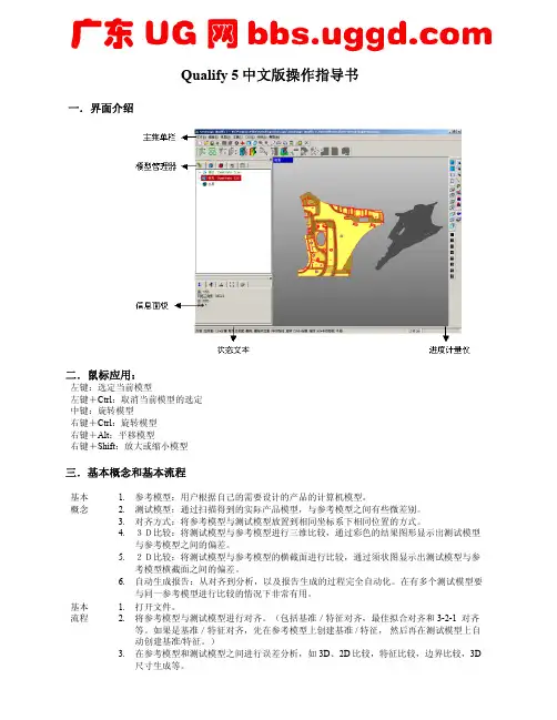
Qualify 5中文版操作指导书一．界面介绍二．鼠标应用：左键：选定当前模型左键＋Ctrl ：取消当前模型的选定中键：旋转模型右键＋Ctrl ：旋转模型右键＋Alt ：平移模型右键＋Shift ：放大或缩小模型三．基本概念和基本流程1. 参考模型：用户根据自己的需要设计的产品的计算机模型。

2.测试模型：通过扫描得到的实际产品模型，与参考模型之间有些微差别。

3.对齐方式：将参考模型与测试模型放置到相同坐标系下相同位置的方式。

4.３Ｄ比较：将测试模型与参考模型进行三维比较，通过彩色的结果图形显示出测试模型与参考模型之间的偏差。

5.２Ｄ比较：将测试模型与参考模型的横截面进行比较，通过须状图显示出测试模型与参考模型横截面之间的偏差。

基本概念 6.自动生成报告：从对齐到分析，以及报告生成的过程完全自动化。

在有多个测试模型要与同一参考模型进行比较的情况下非常有用。

1.打开文件。

2. 将参考模型与测试模型进行对齐。

（包括基准／特征对齐，最佳拟合对齐和3-2-1 对齐等。

如果是基准／特征对齐，先在参考模型上创建基准 / 特征， 然后再在测试模型上自动创建基准/特征。

）基本流程 3.在参考模型和测试模型之间进行误差分析，如3D 、2D 比较，特征比较，边界比较，3D 尺寸生成等。

4. 创建报告。

5. 自动生成报告。

四．Qualify 5操作流程演示：１．打开文件“\…\Geomagic Qualify 5\TutorialData\ sheet-metal-inspection.wrp”。

该文件包含一个CAD模型作为参考模型，以及一个点模型作为测试模型。

在下面的步骤中，将把测试模型与参考模型进行比较，从而得出它们之间的误差。

２．点击“模型管理器”中的“参考－Sheet Metal – CAD”，使当前操作仅对该模型起作用，选择“视图”菜单下的“将整个模型投影到视窗中”命令以及“预定义视图”中的“前视图”命令，将模型放置到便于操作的位置，如下图所示。

GlyphWorks Quick Start Guide2.2Copyright: © nCode International 2005234G l y p h W o r k s 2.2—I n t r o d u c t i o nHow to use these tutorialsWelcome to the ICE-flow GlyphWorks 2.2 tutorials. This introduction covers: • Conventions used in the tutorials• How to get more information from the GlyphWorks online documentation • An overview of the contents of each tutorialIntroduction5IntroductionThere are 5 tutorials designed to get you quickly up to speed with the GlyphWorks 2.2 advanced engineering software. These tutorials are designed to get you up and running via a series of step by step procedures.By working through the tutorials you will learn how to use the advanced functionality of GlyphWorks. More importantly you will learn how to process data files and carry out fatigue analyses.The tutorials should take about an hour each to complete and assume no prior knowledge of GlyphWorks or other nCode products such as nSoft.Each tutorial builds on what you learned from the previous tutorials, so you should do them in sequence. For example, the input file used in the fatigue analysis in tutorial 4 is produced at the end of tutorial 3.Conventions used in the tutorialsThe page layout of the tutorials is designed for ease of navigation: the procedures to follow are shown in the green panel, while more detailed explanations of the analysis and screen shots are shown in the body of the document.The procedure Panel gives concise instruc-tions on what glyphs and files to choose , and what analysis options to use in the examples.A description and intro-duction to the work and analysis is contained in the main body of thedocument along with rele-vant screen shots to help you through the analysis.Information panels give you theory and a conceptual background to the tutorial.Where you see this icon there is a link tomore detailed GlyphWorks helpIntroduction6Getting more information!GlyphWorks (which is a part of the ICE-flow suite of programs) has comprehensive online documentation (over 800 pages of it). We have put signposts into the online documentation pointing to where you can get further information about the topic you are doing. For example:How to access the GlyphWorks online documentationThe on-line documentation is available from within GlyphWorks. •You can view the GlyphWorks manual by selecting from the menu ‘Help | On-line Manual ’ .•Alternatively you could view the entire collection of ICE-Flow manuals by select-ing the Help submenu from the left hand side applications bar and select the Con-tents document.•The document intro_help.pdf tells you how to locate any information in their 800 pages using Adobe Acrobat’ssearch feature.See glyphref.pdf page 27 for more detailIntroductionFurther TrainingAs its name suggests, this guide is intended as a Quick Start into GlyphWorks. Whilst preparing the guide I have tried to introduce each topic by a brief technical description of the analysis being undertaken. This guide is aimed at expert fatigue engineers and students alike, but if anyone would like more detailed information on these topics con-sider doing one of the GlyphWorks training courses. More information about them can be found on the nCode website or by contacting nCode.Introduction78G l y p h W o r k s 2.2—T u t o r i a l 1Data import and displayLearning objectivesThis tutorial shows you how to operate the GlyphWorks 2.2 interface, and how to carry out essential tasks.The topics are:Topic 1 – Learning about test names and channel namesTopic 2 – Starting a GW project—an introduction to the GlyphWorks interface Topic 3 – Displaying data files in GlyphWorks—Glyphs and their properties Topic 4 – Carry out a simple rainflow analysis—using multiple glyphs in a flow Topic 5 – Exporting data from GlyphWorks to an ASCII CSV file for use in MS ExcelTopic 6 – Importing data into GlyphWorks from an ASCII CSV filePre-requisitesICE-flow GlyphWorks 2.2 must be installed on your PCThe following tutorial files must be installed in your working directory. Vib01.dac to vib05.dac Strainrosette.csvTutorial 1—Data Import and Display in GlyphWorks9Tutorial 1—Data Import and Display in GlyphWorksTopic 1In this topic we learn about some standard file naming techniques that you can use to make your data analysis flow more easily. We introduce the concept of breakingdown data in the form of ‘Tests’ and ‘Channels’GlyphWorks can handle all sorts of data from a simple single channel test to a complex multi-test multi-channel configuration. If you only measure small amounts of data then this functionality is probably irrelevant, but if you handle lots of measured data and need to process it automatically then this will save you hours of work.Developing a Test ProgramSuppose we are designing a new anti-roll bar (or sway bar) for a car. We need to make sure that the anti-roll bar works properly on all road surfaces, under all loading conditions from a single occupant to fully laden.To make sure we have covered all eventualities we develop a testing program that measures the response of our anti-roll bar for each ‘Event’ that it might see. Our test program might look something like this:-Now we could choose to measure all the events in one long time signal but we often prefer to separate them into separate test files so it’s easier to see how the anti-roll bar responds to each event. We can either separate them as we measure them, starting a new file just before each test, or we can use GlyphWorks to separate them later.What Are Channels?Once we have determined the Tests we wish to perform over all the various events that our roll-bar is expected to see, we must determined what parameters we want to measure. In this example we might observe the vertical displacement at each wheel along with the torque in the bar. To do this we need twoextensometers for displacement and probably four strain gauges to calculate the torsion. We therefore need to measure 6 channels of simultaneous data as given below:-File Naming Convention:GlyphWorks is designed to handle this sort of data automatically. If you give it a number of tests as input, it will process each of them in turn. Each test, however, can comprise a number of channels of simultaneous measurements and these are all processed simultaneously by GlyphWorks. This makes it really easy therefore to take the raw strain channels obtained above and run them through an equation to derive the torsion moment. GlyphWorks can automatically determine the channel numbering from the file naming convention or from the raw data acquisition files. If the data filenames ends with a pair of numbers then GlyphWorks assumes that these are the channel numbers as shown here. This allows up to 99 channels per test. You can change the properties if you need touse more channels, i.e. 999, 9999, etc... Test Number SurfaceRoad Speed Weight % 01 Smooth straight road 50 50 02 Slow curve 50 50 03 Belgium block 30 50 04Etc...ChannelNumber Transducer01 Vertical Displacement Offside Wheel [mm] 02 Vertical Displacement Nearside Wheel [mm] 03 Torsion Strain Gauge 01 [µε] 04 Torsion Strain Gauge 02 [µε] 05 Torsion Strain Gauge 03 [µε] 06Torsion Strain Gauge 04 [µε]…\TestName02.dac …\Test0102.dacVarious tests shown as folders in a tree Expanding on the test will show each channel of measured data. You can pick 1 channel at a time or process all chan-nels simultaneously.10Property Editor:This shows the calculation properties of the selected Glyph. Each calcula-tion Glyph has a number of properties depending on the type of calculation it performs. Most ofthese are set to sensible defaults by GlyphWorks;however, the user might want to change these for a particular calculation.You can make the property editor larger by drag-ging it’s frame. Alternatively, the property editor is used so regularly that we can view a full sized version by right clicking on the required Glyph and selecting Properties from the menu. (See later examples)Topic 2In this topic we launch the GlyphWorks pro-gram and setup a project folder containing example data for later analysis. •Create a new working directory on your computer and copy the training files here.• Start the ICE-flow GlyphWorks pro-gram•Select the working directory you have just created as your new project folder•Click the GlyphWorks application button from the application toolboxGlyphWorks offers you a choice of project folder. This is the loca-tion on the hard disk where all data pertaining to this project isstored. When GlyphWorks is running you can pick measured data from any input source; hard disk, network or Library data manage-ment system. The folder chosen here is used for GlyphWorks to store any working data you produce.Application Toolbox:nCode GlyphWorks is a suite of engi-neering applications. Each application is launched from the toolbox positioned along the left hand edge of the screen. Applications are grouped logically to help you find the tools you need.Analysis History:This shows the history of things done in GlyphWorks so far and is used for undo and redo functions.Diagnostics and Progress: This shows a detailed account of the calculation progress so far and any errors or warnings found in the calculation process. It helps the user fix any problems quickly and determine how long a complicated calculation is likely to take. Analysis Workspace:This is the workspace where you create your analysis process. Analysis proc-esses are created by dragging calcula-tion Glyphs from the Glyph Palette and dropping them onto the workspace.These are then linked by Pipes to create a calculation flow.Glyph Palette:This palette contains the actual calculation Glyphs. These are dragged onto the workspace to construct the analysis process.Available Data Tree :This tree lists all the available data files for analysis. GlyphWorks will auto-matically load all files in the project folder. The user can add additional files to the tree using the menu ‘File | Open Data Files…’Data files listed here can originate from many sources including the hard disk, network or a Library data management system. They do not have to be stored locally in the project folder. The tree merely stores a link to the original data so you can find it quickly and easily.Tutorial 1—Data Import and Display in GlyphWorksAvailable Data, Tree or Table View:The available data pane can be viewed as either a tree or a table. The tree resembles a standard directory tree, only GlyphWorks allows data to be re-grouped in different ways to improve search-ing. The tree branches can be re-grouped by right clicking on the tree. The following options are available:1. Type of data, followed by test name followed bychannel2. Type of data, followed by channel followed by test3. Disk directory name, followed by test followed bychannelThe available data can also be displayed in tabular format as shown here. In this view, the data can be sorted in different ways by clicking on the appropriate column title. The tabular viewshows more information than the tree view; however, most people find the tree view clearer.These buttons are used to add or remove all tests.The selected tests and chan-nels are shown in this pane. These are imported into GlyphWorks by clicking the ‘Add to File List’ button.Tutorial 1—Data Import and Display in GlyphWorksTopic 3In this topic we look at some typical measured stress data within GlyphWorks.•From the Available data tree, expand the ‘Time Series ’ branch and find the data called ‘vib(dac)’.• Expand ‘vib(dac)’ to see all 5 data channels. •Drag ‘vib(dac)’ onto the work space to create a new Time Series input Glyph and click the Display option to see the plots. •Press the Glyph Maximize button to makethe display full screen•Use the mouse and Tool box to zoom in and out of the plots. Notice the horizontal slider bar over the plot and see how you can scroll through the data by moving it.•Experiment with Cursor coordinates optionon the Tool bar. Click on the plot and read various data values.•Use the ‘Next / Previous Channel’ buttons to navigate through all the channels. Notice there are 5 channels in this data.• Try using overlay and cross plots from the Tool bar.• Use the properties option to display all 5 channels simultaneously.•Zoom-in on a small region of data and ex-periment with the different line stylesfrom the properties options. •When you are quite comfortable with thegraphics options go to the next task.You can drag data directly from the data tree onto the workspace. GlyphWorks automatically recognises the type of data and provides the appropriate data import Glyph.The Time Series Glyph has a preview ‘Display ’ option that provides an interactive plot of the data on the Glyph. This can be viewed full screen by pressing the Glyph maximize button in the top right hand corner of the Glyph.You can zoom in on a block of data by simply clicking either side of the area you are inter-ested in or by dragging the mouse over a win-dow of data. All chan-nels will automatically zoom in on the time interval chosen.Full plotFull X or YRound Y axis to nearest whole numberSwitch between Log and linear axesZoom in-out on X and Y axesMost commonly used graphical display options are available from the tool bar shown below. This will allow you to quickly zoom on the full plot or zoom in and out in stages. You can scroll through your data and change the axes between log and linear. You can also scroll through multiple data channels using the ‘Next / Previous channel’ buttons.Graphical Display ToolTutorial 1—Data Import and Display in GlyphWorksSeparate, overlay or cross-plot multi-ple channelsCursor tracking ofdata pointsChange font sizeSelect or de-select all datapointsRefreshShow cursor coordinatesScroll bar on/offNext / previouschannelNext / previoussection of dataChannels can be incre-mented / decremented in order by one channel at agroup would be 5-8.Frequently used graphical options are shown on the tool bar while the remaining options can be found in the Glyph properties panel byright clicking on the plot and selecting ‘Properties…’ from the menu. The Plotting options are listed under the ’XY Graph ’ tab as shown below.The properties are all listed under generalized headings shown in the left hand tree menu. Click the heading required and the avail-able properties for that appear in the right hand pane. Press the ’OK’ button to apply the properties.Style Options:These let you edit the appearance of the graphical plots. Channels can be shown separately, overlaid on the same axes, or as a cross plot of two channels showing the value of one on the X axis and theother on the Y axis.You can display up to 8 channel plots in one display; although the default is usually set to 4. You toggle between successive channels using the ‘Next / Previous Channel’ buttons.Various axis, grid and colour options are also available from this form.Data Lines:This allows you to change the appearance of the plot. You can change colour, pen thickness, the style of line and the shape of any markers used. Markers are used to highlight the data making it easier to distinguish between channels. Markers do not repre-sent measured points on the data as there are usually too many to plot neatly. However, you can choose the ‘Points’ option to show the actual measured points if required.Labels:To change the label headings, fonts and the style of numbering.Tutorial 1—Data Import and Display in GlyphWorksAxis Limits:These allow you to vary the format and limits of the axes. The for-mat can be Log or Linear, and the limits can be set precisely by entering the desired range.Topic 4In this topic we set up a very simple rainflow analysis and view the results in a 3D histogram. We learn how to use analysis Glyphs with Pipes to channel data through a calculation. •Using the data you loaded in the previous task, drag the ‘Rainflow Cycle Counting ’ Glyph onto the workspace and connect this to the ’Time Series Glyph’ from the previous topic.•Drag a ‘Histogram Display ’ Glyph on to the workspace and connect this to the output of your ‘Rainflow Cycle Counting’ Glyph. Right click on the Rainflow Glyph and select ‘Properties…’ from the menu. Look at the various options available. Right click on any option and select ‘Help on Property…’ from the menu to see what this option means. Don’t worry if you don’t understand some-thing at this stage, we’ll consider the Rain-flow Glyph in greater detail later. • Run the process to see the rainflow matri-ces•Maximize the Histogram Display andchange its properties to show a single chan-nel.• Rotate the 3D histogram by dragging the mouse and see how it follows the mouse. •Use the toolbar buttons to see the differentplotting options available.Input data flows into the GlyphOutput data flows out of the GlyphInput pads on the leftOutput pads on the rightAll connectors are colour coded to represent the type of data that passes through themUsing Glyphs and Pipes:Glyphs are pictorial representations of analysis components. There are input Glyphs, output Glyphs and various function Glyphs. Input Glyphs provide a source of data, like a link to a time history file; Output Glyphs provide a sink for the data, either by graphically displaying the data or by writing to the file system, and Function Glyphs take raw data in and pass process data out.Glyphs are linked together using Pipes connected to pads on the Glyphs themselves. Data flows into a Glyph through the left hand pad and flows out through the right hand pad.Input Glyphs only have pads on the right and output glyphs only have pads on the left.Pads are colour coded to represent the type of data that flows through them, The colour codes are shown below. Pipes can only be used to connect like coloured pads. (Note Grey pads can take any data.)To link two pads with a pipe simply click on one of the pads to be joined, GlyphWorks will then highlight all the compatible pads on the other Glyphs. Simply move the mouse over the other pad and click on it.Pipes can be removed by right clicking on the pipe and selecting ‘Disconnect’ from the menu. Alternatively, pipes are automatically removed if you delete a Glyph.Quick Tip: You can drag a Glyph from the Glyph palette and drop it on the pad of another Glyph. This will automatically create a pipe between them if they are compatible.Blue RedGreenGrey Time Series DataHistogram DataMetadataAny Data TypeColour conventions used for PadsMaximize PlotTutorial 1—Data Import and Display in GlyphWorksAdvanced Properties:These options are available by right clicking on the plot and se-lecting the ‘Properties…’ option from the menu. The advanced property form is similar to that seen earlier for the Time History Display; however, you’ll notice some features specific to 3D plotslocated on the ’Styles—Plots’ option shown below.Viewing Options:Isometric, top, left & rightView as block histogram or surface plot Full PlotScale all plots to the same axislimitsChange font sizeSelect or de-select all datapointsNext / previouschannelChannels can be incre-mented / decremented in order by one channel at a time or by groups of chan-nels. So if channels 1-4 are currently showing, the next group would be 5-8. The mode of increment / decrement is chosen by holding the button down and then picking from themenu shown.Top view of a Surface plotThe number of displays shown on each plot can be changed from this option form.The rotation angle and zoom can also be selected here. This is changed interactively by dragging the mouse over the plot; how-ever, more control is offered by allowing the user to type in the numerical angle required.The graph can be shown using histogram towers or as a surface plot while colours can be used in different ways to enhance the display.Tutorial 1—Data Import and Display in GlyphWorksTo interactively Rotate the Graph, simply left click on the plot and drag the mouse in the direction required.3D Histogram DisplayThe rainflow results are shown using the 3D histogram display Glyph. This can display up to 8 interactive histograms in one dis-play. The Glyph automatically configures the display to show up to 4 plots for multi-channel data. The number of plots shown can be changed using the Advanced Properties options (right click).Maximize the plot by clicking on the button in the top right hand cor-ner of the Glyph. A typical plot is shown below. It can be rotated by clicking and dragging the mouse. The most common options are provided on the Tool bar shown at the bottom of the page. If you get a little lost after dragging, press the ‘Isometric’ button to return to normal. Another useful option is the ‘Top’ view option. This makes for a particularly pleasing graph when used in conjunction with the ‘Surface’ option.Hint: If you want to clear the input files and look at another set of data then simply right click on the TSInput Glyph and select ‘Remove Tests’ from the menu. You can now drag another set of data from the Available data tree and drop them on the TSInput Glyph.You can also drop several tests on the TSInput Glyph at once; however, you can only view one test at a time.Topic 5In this topic we export Data to both Binary and ASCII output files. •Using the GlyphWorks process created in the topic 3, add the Histogram Out-put Glyph and rerun the process. •Edit the GlyphWorks process and add a Data Value Display Glyph. Export the histogram to a CSV file and look at this file in MS Excel.•Edit the GlyphWorks process and view the numerical values of all channels in the input time series using the ValueDisplay Glyph.Binary Data Output:Output data from GlyphWorks can be written in a file for later use by other programs. This might be report generation using ICE-flow Studio, test rig drive signals, input to FE-Fatigue analysis or Multi-body simulation, etc.Binary data is output using the appropriate output Glyphs; these being Time Series, Multi-column or Histogram data.By default, the Output Glyph uses the same filename as the input but appends ‘_out’ to the end of the filename. You can change the output name via the Glyph Properties. Right click on the Glyph andselect ‘Properties’ to get the following options:Select type of Binary format to use: either DAC or S3 format.Meta data can also be stored with the plot. Metadata contains information on the settings used in the analysis as well as statistical quanti-ties and titles and units.GlyphWorks can be instructed to automatically overwrite existing files or Ask for user confirmation first.The new data can be added auto-matically to the Data tree if required; otherwise the user must press the data refresh button to load the new data.The output filename is automatically assigned based on the following options: 1. Use existing filename with a given suffix 2. Use existing filename with a given prefix 3. Use a new filename 4. Use the existing filename but write to another directoryTutorial 1—Data Import and Display in GlyphWorksASCII Data Output:Data can also be written to ASCII files for use by programs that can-not read Binary files; these include FE analysis packages, Spread-sheets, Mathcad, Matlab, etc.ASCII data is output using the ‘Data Values Display’ Glyph. This can be used to give a numerical view of the data on screen but is also able to output to CSV (Comma Separated Values) files by clicking the ‘Export’ button on the Glyph. The user is prompted for a file-name.The Data Value Glyph does not show all data points by default but instead shows 1 in 10 points. This default can be over-ridden usingthe right-click ‘Properties…’ option.Enter the channels to export. Channel numbers can be written as a comma sepa-rated list or using a range of channels expressed in the form; ‘1-3’ , etc...Select the preferred bin labels for histogram data. Cells can be labelled using the centre value or the minimum value covered by the bin.Enter the number of significant figures to use for each value. Internally GlyphWorks main-tains a precision of approxi-mately 12 significant figures but this is probably excessive and can result in large file sizes.This only applies to Time Series and Multi-column data. Data might not be required for all values in a time series so this allows the user to select to output every 10th point or every 1 sec-ond for example.Remember you can view help on any of these options by right-clicking on the option and selecting ‘Help on Property…’ from the menu.Tutorial 1—Data Import and Display in GlyphWorksdata in the same format you can save your translation settings The CSV file shown here contains measured Time Series strainEnter ASCII filename for translation. This can con-tain any format of ASCII data including CSV(Comma Separated Val-ues), Space separated, tab separated, etc.Time Series files have no separate time axis. The time for each point is calculated knowing the starting time (Base Time) and the constant Sam-ple Rate.Multi-column files have a separate time axis that doesn’t have to be measured at a constant sample rate and may also contain a date column for long term measured data.Wizard values and automate the translation. The option to save a setup file is offered on the final wizard form.Header lines are included at the top of most ASCII files to describe the data present and provide other information like the sample rate, units, etc. ASCII Translate needs to know how many header lines are pre-sent so it doesn’t confuse these with the actual measured data. It can also use some of this data to automatically assign units and titles to the plots.There are many ways of formatting ASCII files and it is unfeasible to detect the format automatically. ASCII Translate provides a data preview window so the user can choose the formatting options from the ’Fields’ and see whether these are satisfactory.Tutorial 1—Data Import and Display in GlyphWorksTime Series data does not contain a separate time column so the user must enter the Sample rate and time base (starting time). The actual time values for each point can then be calculated.The user can change the label and units used for the X-axis. By default these are assumed to be Time meas-ured in Seconds.ASCII Translate produces a binary output file that can be used di-rectly by GlyphWorks. GlyphWorks can read a number of binary formats and the user can select the preferred format and filename. The filename defaults to the original ASCII filename while the format defaults to the GlyphWorks standard format. The choice of format largely depends on the user’s requirements and is discussed in the information box opposite.At the end of the translation a summary log is produced so you can make sure everything went as expected. You also have the option to Save the Setup file so you can re-run the conversion quickly on other similar files.Translating Multi-column data:Multi-column data always requires a time column and optionally a date column where data is measured over a long period of time.The translation process is the same as for Time Series data except a Wizard form is offered for you to enter whether the data contains date as well as time, and the date formatting used. You must also enter which columns pertain to the time and date.Tutorial 1—Data Import and Display in GlyphWorks。