傅里叶级数下连续小推力(译文)
- 格式:doc
- 大小:5.01 MB
- 文档页数:24
离散傅里叶级数推导标题:离散傅里叶级数(DFS)的推导与理解一、引言离散傅里叶级数(Discrete Fourier Series,简称DFS)是信号处理和数据分析中一种强有力的工具,它将周期性离散信号分解为一系列简单正弦波和余弦波的线性组合,从而揭示出信号内在的频率结构。
本篇文档旨在详细阐述离散傅里叶级数的理论基础及其推导过程。
二、离散傅里叶级数基本概念离散傅里叶级数主要应用于周期为N的离散时间信号f[n],其表示形式如下:f[n] = a0 + Σ(ak * cos(2πkn/N) + bk * sin(2πkn/N))其中,k=1, 2, ..., (N-1),a0, ak, bk分别代表直流分量和交流分量系数。
三、离散傅里叶级数的推导1. **直流分量**:a0是信号的平均值,可通过求信号序列的平均值得到,即a0 = (1/N) * Σf[n] (n=0,1,...,N-1)2. **交流分量系数**:对于每个正弦项和余弦项,其系数ak和bk可以通过内积运算得到,具体公式如下:ak = (1/N) * Σf[n] * cos(2πkn/N)bk = (1/N) * Σf[n] * sin(2πkn/N)3. 整体推导:将上述各系数代入原始的离散傅里叶级数表达式,即可完成从原始离散信号到其傅里叶级数展开式的转换。
四、离散傅里叶级数的应用与特性离散傅里叶级数不仅提供了一种分析周期信号的方法,还具有诸多重要性质,如频谱对称性、能量守恒性等。
在实际应用中,例如图像处理、音频压缩、数字通信等领域,DFS都有广泛的应用。
五、结论离散傅里叶级数作为数学工具在工程领域中的重要地位不言而喻,通过对其深入理解和推导,我们可以更有效地进行信号分析与处理,揭示并利用信号的内在规律。
对于复杂系统的设计与优化,离散傅里叶级数无疑是一种不可或缺的基础理论支撑。

实验三 连续时间傅立叶级数成谐波关系的复指数信号就是它们的频率互为整数倍的信号,傅立叶级数将周期信号表示成谐波关系的复指数信号的加权和,如(3.1)和(3.2)式。
因为复指数信号是LTI 系统的特征函数。
所以这种表示能够直接计算在一给定周期输入下一个系统的输出.∑∞-∞==k tkf j p ek X t x 02][)(π (3.1)⎰-==Ttkf j p tet x Tk X d )(1][02π (3.2)§3.1 连续时间傅立叶级数的性质 目的本练习要检验连续时间傅立叶级数(CTFS )的性质。
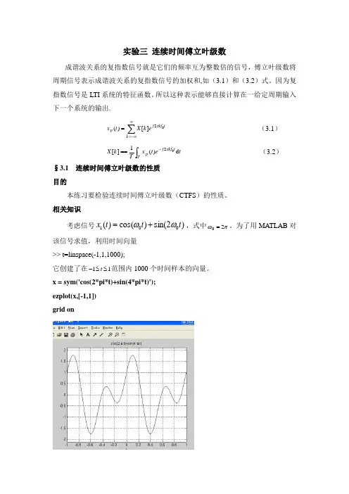
相关知识考虑信号)2sin()cos()(001t t t x ωω+=,式中πω20=。
为了用MATLAB 对该信号求值,利用时间向量 >> t=linspace(-1,1,1000);它创建了在11≤≤-t 范围内1000个时间样本的向量。
x = sym('cos(2*pi*t)+sin(4*pi*t)'); ezplot(x,[-1,1]) grid on中等题1. 满足)()(11T t x t x +=的最小周期T 是多少?利用这个T值,用定义求)(1t x 的CTFS 系数。
从图中可知最小T 为0.82.考虑信号)()()(11t x t x t y -+=,利用CTFS 的时间倒置和共轭性质求)(t y 的CTFS系数。
3.在11≤≤-t 上画出信号)(t y 。
能预计出什么样的对称性?能够利用CTFS 的对称性说明它吗? 4.考虑信号)()()(*11t x t x t z -=。
利用CTFS 的时间倒置和共轭性质求)(t z 的CTFS系数。
§3.2 连续时间傅立叶级数中的能量关系 目的分别在时域和频域求信号能量,验证帕斯瓦尔定理。
相关知识一个硬限幅器是一种器件,其输出是即时输入信号符号的函数,具体说就是当输入信号)(t x 是正时,输出信号)(t y 等于1;而当)(t x 是负时,输出信号)(t y 等于-1。
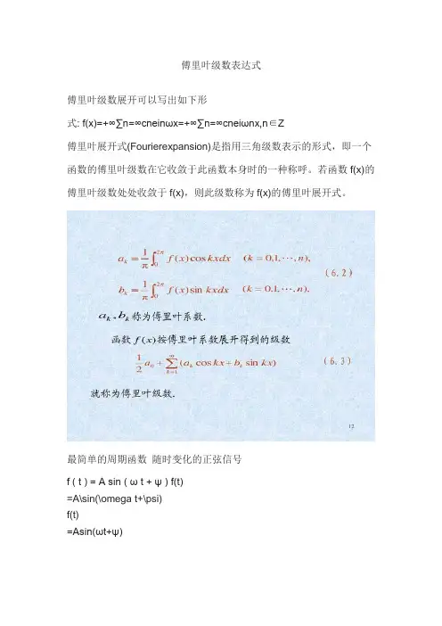
傅里叶级数公式傅里叶级数展开傅里叶级数收敛性的计算公式傅里叶级数公式的计算公式提供了一种将任意周期函数表示为一组正弦和余弦函数的和的方法。
这种表示方法在信号处理、图像处理等领域具有重要应用。
在本文中,将详细介绍傅里叶级数展开和收敛性的计算公式。
一、傅里叶级数展开傅里叶级数展开是将周期为T的函数f(t)表示为一组三角函数的和。
傅里叶级数展开的计算公式如下:f(t) = a0 + Σ (an*cos(nωt) + bn*sin(nωt)),其中a0、an和bn分别为系数,ω为角频率,n为正整数。
根据这个公式,我们可以将任意周期函数表示为一组正弦和余弦函数的和。
傅里叶级数展开的关键是计算系数a0、an和bn,这里不再赘述具体的推导过程。
二、傅里叶级数收敛性的计算公式傅里叶级数的收敛性是指在何种条件下,傅里叶级数能够无限接近原函数f(t)。
傅里叶级数的收敛性可以通过计算系数a0、an和bn来确定。
1. 正弦级数的收敛性对于奇函数,即满足f(-t)=-f(t)的函数,其傅里叶级数只包含正弦函数。
对于奇函数f(t),其傅里叶级数的计算公式为:f(t) = Σ (bn*sin(nωt)),其中bn的计算公式为:bn = (2/T) * ∫[0,T] {f(t)*sin(nωt)} dt。
当函数f(t)满足一定的条件时,傅里叶级数对奇函数收敛。
这些条件包括函数f(t)在一个周期内有有限个有界不连续点,并且在这些点上的左右极限存在。
2. 余弦级数的收敛性对于偶函数,即满足f(-t)=f(t)的函数,其傅里叶级数只包含余弦函数。
对于偶函数f(t),其傅里叶级数的计算公式为:f(t) = a0/2 + Σ (an*cos(nωt)),其中a0和an的计算公式为:a0 = (2/T) * ∫[0,T] {f(t)} dt,an = (2/T) * ∫[0,T] {f(t)*cos(nωt)} dt。
同样地,当函数f(t)满足一定的条件时,傅里叶级数对偶函数收敛。
傅里叶级数帕塞瓦尔定理
傅里叶级数帕塞瓦尔定理是一个多项式的公式,用来解释特定序
列(波形)的行为。
它是由法国数学家Joseph Fourier在1807年提
出的,用于将某种信号建模。
该定理可以应用于任何有限或无限冲激
响应(LTI)系统,如电路和比例控制系统,用于分析它们的性能。
它
也可以应用于多元式非线性系统,用于解释sysrem的行为,即系统中
不同输入变量对输出变量的影响。
实际上,傅里叶级数帕塞瓦尔定理可以描述任何一个连续函数,
当它作为周期函数时,它的形状可以被表示为若干函数的有限和不断
的级数,即傅里叶级数(Fourier Series)。
这些函数可以是正弦波、余弦波或者生成函数。
因此,傅里叶级数可以将任意定义的连续函数
表示为和不同频率成正比的正弦和余弦波(Sin x 和 Cos x )的组合,而且可以通过傅里叶级数来估计函数在不同点的值。

傅里叶级数表达式
傅里叶级数展开可以写出如下形
式: f(x)=+∞∑n=∞cneinωx=+∞∑n=∞cneiωnx,n∈Z
傅里叶展开式(Fourierexpansion)是指用三角级数表示的形式,即一个函数的傅里叶级数在它收敛于此函数本身时的一种称呼。
若函数f(x)的傅里叶级数处处收敛于f(x),则此级数称为f(x)的傅里叶展开式。
最简单的周期函数随时变化的正弦信号
f ( t ) = A sin ( ω t + ψ ) f(t)
=A\sin(\omega t+\psi)
f(t)
=Asin(ωt+ψ)
傅里叶级数
三角函数系的正交性
三角函数系:{1,sinx,cosx,sin2x,cos2x,…,sinnx,cosnx,…},它由无数个sinnx和cosnx组成,其中n=0,1,2,…。
傅里叶就试图将周期为T 的函数f(x) 展开为sinx 和cosx 函数和的形式。
那怎么保证组合出来的函数周期依然为T 呢?
函数f=sinωt 的周期为T′=2πω,要使得原函数能够被三角函数表示,那么三角函数的粒度必然要小于原函数,即三角函数的最小周期T′ 必须小于原函数f(x) 的最小周期T,即
2πω≤T2πnω=T,n>0。
傅里叶级数第八节傅里叶级数内容分布图示★ 引言★ 引例★ 三角函数系的正交性★ 傅里叶级数的概念★ 狄利克雷收敛定理★ 例1 ★ 例2 ★ 例3★ 非周期函数的周期延拓★ 例4 ★ 利用傅氏展开式求数项级数的和★ 正弦级数与余弦级数★ 例5 ★ 例6★ 函数的奇延拓与偶延拓★ 例7 ★ 例8★ 内容小结★ 课堂练习★ 习题11-8★ 返回讲解注意:一、三角级数三角函数系的正交性早在18世纪中叶,丹尼尔. 伯努利在解决弦振动问题时就提出了这样的见解:任何复杂的振动都可以分解成一系列谐振动之和. 这一事实用数学语言来描述即为:在一定的条件下,任何周期为T )/2(ωπ=的函数)(t f ,都可用一系列以T 为周期的正弦函数所组成的级数来表示,即∑∞=++=10)sin()(n n n t n A A t f ?ω (8.1)其中n n A A ?,,0),3,2,1( =n 都是常数.十九世纪初,法国数学家傅里叶曾大胆地断言:“任意”函数都可以展成三角级数. 虽然他没有给出明确的条件和严格的证明,但是毕竟由此开创了“傅里叶分析”这一重要的数学分支,拓广了传统的函数概念. 傅里叶的工作被认为是十九世纪科学迈出的极为重要的第一个大步,它对数学的发展产生的影响是他本人及同时代的其他人都难以预料的. 而且,这种影响至今还在发展之中. 这里所介绍的知识主要是由傅里叶以及与他同时代的德国数学家狄利克雷等人的研究结果.二、函数展开成傅里叶级数傅里叶系数====??--).,3,2,1(,sin )(1),,2,1,0(,cos )(1 n nxdx x f b n nxdx x f a n n ππππππ (8.5) 将这些系数代入(8.4)式的右端,所得的三角级数∑∞=++1)sin cos (2n n n nx b nx a a (8.6)称为函数)(x f 的傅里叶级数.定理1(收敛定理,狄利克雷充分条件)设)(x f 是周期为π2的周期函数. 如果)(x f 满足在一个周期内连续或只有有限个第一类间断点,并且至多只有有限个极值点. 则)(x f 的傅里叶级数收敛,并且(1) 当x 是)(x f 的连续点时, 级数收敛于)(x f ;(2) 当x 是)(x f 的间断点时, 收敛于2)0()0(++-x f x f .狄利克雷收敛定理告诉我们:只要函数)(x f 在区间],[ππ-上至多只有有限个的第一类间断点,并且不作无限次振动,则函数)(x f 的傅里叶级数在函数的连续点处收敛于到该点的函数值,在函数的间断点处收敛于该点处的函数的左极限与右极限的算术平均值. 由此可见,函数展开成傅里叶级数的条件要比函数展开成幂级数的条件低得多.三、周期延拓:在区间),[ππ-或],(ππ-外补充)(x f 的定义,使它拓广成一个周期为π2的周期函数)(x F ,这种拓广函数定义域的方法称为周期延拓.四、正弦级数与余弦级数:一般地, 一个函数的傅里叶级数既含有正弦项, 又含有余弦项(例2),但是, 也有一些函数的傅里叶级数只含有正弦项(例1)或者只含有常数项和余弦项(例4),导致这种现象的原因与所给函数的奇偶性有关。
傅里叶级数与傅里叶变换是数学分析中两个重要的概念和理论工具,它们在信号处理、图像处理、物理学等领域有广泛的应用。
傅里叶级数是一种将周期函数分解为一系列谐波的方法,而傅里叶变换是将非周期函数分解成连续谱的方法。
首先,我们来介绍一下傅里叶级数。
傅里叶级数是将一个周期为T的函数f(t)展开为一系列谐波的和的形式,其中每个谐波都有一个特定的频率和振幅。
傅里叶级数的基本公式为:f(t) = a0 + Σ(An cos(nω0t) + Bn sin(nω0t))其中a0表示直流分量,An和Bn分别表示正弦和余弦项的振幅,n为谐波的阶数,ω0为基本频率。
傅里叶级数的系数可以通过求解积分或者利用傅里叶级数的性质进行计算。
傅里叶级数的应用十分广泛。
例如在信号处理中,傅里叶级数可以用来将一个周期信号分解为多个频率成分,从而进行频域分析和滤波等操作。
此外,傅里叶级数也可以用来恢复被损坏的信号,例如在音频和图像压缩中,傅里叶级数可以用来还原被压缩的信号。
接下来,我们来介绍傅里叶变换。
傅里叶变换是将一个非周期函数f(t)分解成连续的频谱。
傅里叶变换的基本公式为:F(ω) = ∫[f(t)*e^(-jωt)] dt其中F(ω)表示函数f(t)在频率ω处的频谱,e^(-jωt)是一个旋转复指数,j为虚数单位。
傅里叶变换的结果是一个连续的函数,其中包含了函数f(t)在不同频率上的振幅和相位信息。
傅里叶变换的应用也非常广泛。
在信号处理中,傅里叶变换可以用来将一个时域信号转换成频域信号,在频域进行滤波、增强和分析操作。
在图像处理中,傅里叶变换可以用来进行图像的频域滤波、边缘检测和压缩等操作。
在物理学中,傅里叶变换可以用来研究波动、振动和量子力学等问题。
傅里叶级数和傅里叶变换是相互联系的。
当一个函数是周期函数时,傅里叶级数可以通过傅里叶变换来计算。
而当一个函数是非周期函数时,傅里叶变换可以通过傅里叶级数来近似计算。
总之,傅里叶级数和傅里叶变换是数学分析的两个重要工具,它们在信号处理、图像处理和物理学等领域具有广泛的应用。
傅⾥叶级数傅⾥叶变换:(频域分析)连续系统频谱分析:就是将时域的信号(可以是周期信号与⾮周期信号)变成频域形式并加以分析的⽅法。
其⽬的是把复杂的时域波形,经过某种变换分解为若⼲单⼀的谐波分量来研究,以获得信号的频率结构以及各谐波和相位信息。
这某种变换可以是傅⾥叶级数,也可以是傅⾥叶变换。
它们的作⽤都是把时域信号变成频域信号以便于信号分析。
傅⾥叶级数有三⾓级数形式和指数级数形式两种表⽰形式。
例如,假设有个周期信号,周期为,⾓频率,频率为。
要作频谱分析时,按傅⾥叶级数展开:三⾓形式的傅⾥叶级数******(a)直流分量:****** (a1)余弦分量幅度:****** (a2)正弦分量幅度:****** (a3)由上可见,公式a左边是⼀个周期信号,⽽右边是⼀个三⾓函数的线性组合,或也可以称为三⾓级数表⽰⽅式,这种三⾓级数的表⽰⽅式就称为傅⾥叶级数。
但公式(a)有个问题,就是说在每个频率点上可能会有两个三⾓函数,这不利于信号能量的计算或图形表⽰,为了便于画图我们做了⼀些变换,⽤三⾓公式中的合⾓公式对公式(a)进⾏了转换,把同频率的项加以合并,于是得到了余弦形式的傅⾥叶级数或正弦形式的傅⾥叶级数,如式(b),(c)。
余弦形式:****** (b)正弦形式:****** (c)由上总结:1、⼀个周期信号可以分解成直流分量、基波()和各次谐波(基波⾓频率整数倍)的线性组合。
2、周期信号频谱具有离散型,谐波性,收敛性。
为幅度频谱关系由此可画出频谱图为相位频谱关系欧拉公式:****** (d1)****** (d2)将公式(d1)、(d2)带⼊公式(a)可得:****** (d3)**** (d4)**** (d5)将公式(d4)、(d5)带⼊(d3)可得:****** (d6)令:****** (d7)从⽽得到f(t)得到指数形式的傅⾥叶级数:****** (e)将(a2)、(a3)带⼊(d4),其中可以简写成。
重温傅里叶—笔记篇本文记录得大多就是基础得公式,还有一些我认为比较重要得有参考价值得说明、(如果对这些公式已经很熟悉,可以直接瞧第三部分:总结性说明)重温傅里叶—笔记篇一、傅里叶级数$关于三角函数系得正交性:三角函数系包括:1, cosx, sinx , cos2x, sin 2x, ……cos nx, sin nx, ……“正交性"就是说,三角函数系中得任何一项与另一项得乘积,在(-π, π) 区间内得积分为0。
(任何两相得积总可以展成两个频率为整数倍基频得正余弦函数之与或差,而这两个展开后得正余弦在(—π,π)上积分都为0)。
不同频率(但都就是整数倍基频)得两个正弦函数之积,在(-π, π)上积分恒为0。
同频率得两个正弦函数之积,只有在这两个正弦得相位正交时,其在(-π,π)上积分才就是0、三角函数系中除“1”以外得任何一项得平方,在(—π,π)上得积分恒为π,“1”在这个区间上得积分为2π。
$上公式!①当周期为2π时:式(1):上式成立得条件就是f(x)满足狄立克雷充分条件:1。
在任意有限区间内连续,或只有有限多个第一类间断点;2. 任意得有限区间,都可被分成有限多个单调区间(另一种说法就是:任意有限区间内只有有限多个极值点,其实就是一样得)式(1)第一行中得a0/2 就就是f(x)得周期平均值,而且第一行得式子只对f(x)就是连续函数得情况成立;如果f(x)不连续,则应表示成“(1/2)×[f(x—0)+f(x+0)]”,即f(x)左右极限得算术平均。
下面得类似情况都就是这样,之后就不再专门说明,这些大家应该都懂。
第三、四行中,n得取值都就是:1,2,3,4,……n,……(都为正,且不包含0)。
②当周期为2L时(这也就是最一般得情形):式(2):第一行中得a0/2 就就是f(x)得周期平均值;第三、四行中,n得取值都就是:1,2,3,4,……n,……(都为正,且不包含0)。
Reduction of Low-Thrust Continuous Controls for Trajectory Dynamics 前言摘要 A novel method to evaluate the trajectory dynamics of low-thrust spacecraft is developed. The thrust vectorcomponents are represented as Fourier series in eccentric anomaly, and Gauss’s variational equations are averaged over one orbit to define a set of secular equations.These secular equations are a function of only 14 of the thrust Fourier coefficients, regardless of the order of the original Fourier series, and are sufficient to accurately determine a low-thrust spiral trajectory with significantly reduced computational requirements as compared with integration of the full Newtonian problem. This method has applications to low-thrust spacecraft targeting and optimal control problems.
一种新的求解小推力轨道动力学的方法被开发出来了。推力向量的各坐标用偏近点角表示为傅里叶级数,并且将高斯变分方程平均到整个轨道上来提高久期方程组的精度。这些久期方程组仅仅是14个推力傅里叶系数的函数而忽略初始傅里叶级的次数,这些方程能够精确有效的解决小推力螺旋轨道问题,且与通常的牛顿问题的积分方法相比能大大减少计算量。这一方法应用在小推力航天器的目标确定和最优控制问题中。
I. Introduction 引言 LOW-THRUST propulsion systems offer an efficient option for many interplanetary and Earth-orbit missions. However, optimal control of these systems can pose a difficult design challenge. Analytical or approximate solutions exist for several special cases of optimal low-thrust orbit-transfer problems, but the general continuous-thrust problem requires full numerical integration of each initial condition and thrust profile. The trajectory is highly sensitive to these variables; thus, the optimal control law over tens or hundreds of orbits of a spiral trajectory is often difficult to determine. 小推力推进系统为许多星际航行和地球轨道任务提供了一种高效的新选择。但是这种系统却对最优化控制提出了新的挑战。对于几种特殊的小推力下的轨道转移的最优控制问题已经出现了解析法和数值近似解的方法,但是对于一般的连续推力问题 需要对每一个初始条件和推力值进行完全的数值积分。轨道参数的确定往往对这些变量很敏感,因此,(普通的)最优控制法则对于确定螺旋轨道的数十甚至上百个轨道是十分困难的。
Analytical solutions have been developed for many special-case transfers, such as the logarithmic spiral [1–3], Forbes’s spiral [1], the exponential sinusoid [4,5], the case of constant radial or circumferential thrust [6–8], Markopoulos’s Keplerian thrust programs [9], Lawden’s spiral [10], and Bishop and Azimov’s spiral [11]. More recent solutions have used the calculus of variations [12] or direct optimization methods [13] to determine optimal low-thrust control laws within certain constraints. Several methods for open-loop minimum-time transfers [14–16] and optimal transfers using Lyapunov feedback control [17,18] also exist. Averaging methods in combination with other approaches have proven to be effective at overcoming sensitivities to small variations in the initial orbit and thrust profile [19–22], yet all solutions remain limited to certain regions of the thrust and orbital parameter space. 在一些特殊情形的轨道转移中,数值解法已经得到了挖掘,如对数螺旋(上升/下降),福布斯螺旋(上升/下降),指数正弦曲线,常值径向/切向推进,马氏开普勒推进,劳登螺旋,毕-阿氏螺旋等。而最新的更多解法则应用变量/变差的微积分或直接优化法来来确定特定约束条件下的小推力最优控制律。一些求解开环(轨道)的时间最优轨道转移和李雅普诺夫反馈最优轨道转移法也早就出现。实践证明,把平均法和其它方法结合的思路在解决对初始轨道/推力变量预测敏感的问题上有很有效的,但所有这些方法都局限于由推力和轨道参数形成的空间区域中。
The focus of this study is a novel method to evaluate the effect of low-thrust propulsion on spacecraft orbit dynamics with minimal constraints. We represent each component of the thrust acceleration as a Fourier series in eccentric anomaly and then average Gauss’s variational equations over one orbit to define a set of secular equations. The equations are a function of only 14 of the thrust Fourier coefficients, regardless of the order of the original Fourier series; thus, the full continuous control is reduced to a set of 14 parameters.
本文研究的重点是提出一种评估/解决带有最少约束的航天器轨道动力学的小推力推进效应/问题。我们将推进加速度向量的各坐标用偏近点角表示为傅里叶级数,并且将高斯变分方程平均到整个轨道上来提高久期方程组的精度。忽略初始傅里叶级的次数,这些久期方程组仅仅是14个推力傅里叶级系的函数,因而整个连续控制问题的参数减少为14个。
With the addition of a small correction term to eliminate offsets of the averaged trajectory due to initial conditions, the averaged secular equations are sufficient to determine a low-thrust trajectory with a high degree of accuracy. This is verified by comparison of the averaged trajectory dynamics with the fully integrated Newtonian equations of motion for a basic step-acceleration function and a randomly generated continuous-acceleration function. 我们用添加小的修正项的方法来消除由于初始条件造成的平均轨道的误差,这样,这个平均轨道就可以有足够的精度来解决小推力轨道(转移)问题。这个已经通过对比平均轨道动力法和基本分步加速度函数及随机连续加速度函数的牛顿运动方程全积分法证实。
The method has certain limits of applicability. First, the thrust acceleration must be able to be represented by a Fourier series, as is true for almost any physical system.