A Linear Algorithm for the Hyper-Wiener Number of Chemical Trees

but if D is diagonal, then E has axes along the coordinate directions and the length of the ith semi-axis is A/d..
i
We now consider the solution of (2.1) in some generality, and thus the problem (2.3) min{IIf+Jpll : IIDpll~ A} The basis for the Levenberg-Marquardt = p(l) for some
THE LEVE_~BERG-MARQUARDT IMPLEMENTATION
ALGORITHM:
AND THEORY
Jorge J. Mor~
i.
Introduction Let F: R n ÷ R m be continuously differentiable, of and consider the nonlinear least
4
ilI] I
where D~ = x½~TD~ is still a diagonal matrix and R is a (possibly singular) upper triangular matrix of order n.
108
In the second stage, compute the QR decomposition (3.4).
squares problem of finding a local minimizer
(1.1)
Levenberg numerical
I ~(x) = 7

f matrices and through a transformation to a product of two symmetric matrices if ∙ ¸ ∙ ¸ 1 −1 0 1 = and = 2 3 −1 2 10. a. Can one use this section’s formulas that indicate the complexity equivalence of multiplication and squaring of integers to show the complexity equivalence of multiplication and squaring of square matrices? b. Show that multiplication of two matrices of order can be reduced to squaring a matrix of order 2 11. Find a tight lower bound class for the problem of finding two closest numbers among real numbers 1 2 ..., . 12. Find a tight lower-bound class for the number placement problem (Problem 9 in Exercises 6.1).
This file contains the exercises, hints, and solutions for Chapter 11 of the book ”Introduction to the Design and Analysis of Algorithms,” 3rd edition, by A. Levitin. The problems that might be challenging for at least some students are marked by B; those that might be difficult for a majority of students are marked by I

ported by FMSTF(2004J024) and NSFF(E0540007). Partially supported by NSC 95-2115-M-001-009. Email address: weigenyan@ (W. G. Yan), mayeh@.tw (Y. N. Yeh).
Enumeration of subtrees of trees
Weigen Yana,b
a
1
and
Yeong-Nan Yehb
2
arXiv:math/0609475v1 [math.CO] 17 Sep 2006
School of Sciences, Jimei University, Xiamen 361021, China
1
(resp. b(T ; vi , vj ; k )) the number of subtrees of T with k vertices, each of which contains vertex vi (resp. vertices vi and vj ). Obviously, for any k = 0, 1, . . . , n − 1, we have the following: a(T ; k ) = b(T ; k + 1), a(T ; vi; k ) = b(T ; vi ; k + 1), a(T ; vi, vj ; k ) = b(T ; vi , vj ; k + 1). For a given subtree T1 of a weighted T , we define the weight of T1 , denoted by ω (T1 ), as the product of the weights of the vertices and edges in T1 . The generating function of subtrees of a weighted tree T = (V (T ), E (T ); f, g ), denoted by F (T ; f, g ), is the sum of weights of subtrees of T . That is, F (T ; f, g ) =

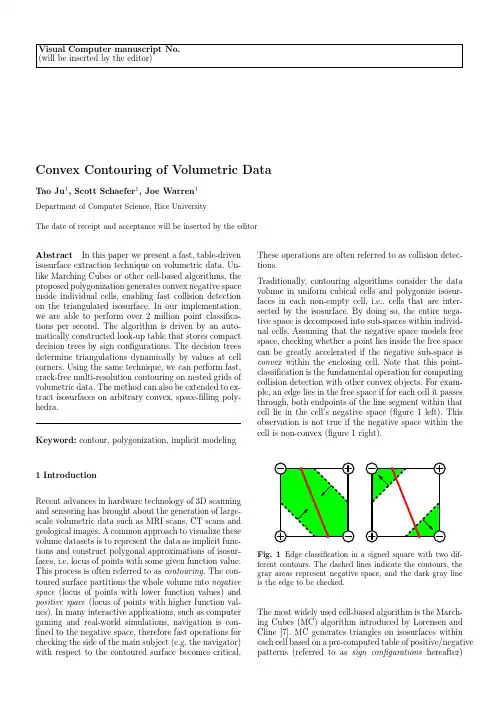
Visual Computer manuscript No.(will be inserted by the editor)Convex Contouring of Volumetric Data Tao Ju1,Scott Schaefer1,Joe Warren1Department of Computer Science,Rice UniversityThe date of receipt and acceptance will be inserted by the editorAbstract In this paper we present a fast,table-driven isosurface extraction technique on volumetric data.Un-like Marching Cubes or other cell-based algorithms,the proposed polygonization generates convex negative space inside individual cells,enabling fast collision detection on the triangulated isosurface.In our implementation, we are able to perform over2million point classifica-tions per second.The algorithm is driven by an auto-matically constructed look-up table that stores compact decision trees by sign configurations.The decision trees determine triangulations dynamically by values at cell ing the same technique,we can perform fast, crack-free multi-resolution contouring on nested grids of volumetric data.The method can also be extended to ex-tract isosurfaces on arbitrary convex,space-filling poly-hedra.Keyword:contour,polygonization,implicit modeling 1IntroductionRecent advances in hardware technology of3D scanning and sensoring has brought about the generation of large-scale volumetric data such as MRI scans,CT scans and geological images.A common approach to visualize these volume datasets is to represent the data as implicit func-tions and construct polygonal approximations of isosur-faces,i.e.locus of points with some given function value. This process is often referred to as contouring.The con-toured surface partitions the whole volume into negative space(locus of points with lower function values)and positive space(locus of points with higher function val-ues).In many interactive applications,such as computer gaming and real-world simulations,navigation is con-fined to the negative space,therefore fast operations for checking the side of the main subject(e.g.the navigator) with respect to the contoured surface becomes critical.These operations are often referred to as collision detec-tions.Traditionally,contouring algorithms consider the data volume in uniform cubical cells and polygonize isosur-faces in each non-empty cell,i.e.,cells that are inter-sected by the isosurface.By doing so,the entire nega-tive space is decomposed into sub-spaces within individ-ual cells.Assuming that the negative space models free space,checking whether a point lies inside the free space can be greatly accelerated if the negative sub-space is convex within the enclosing cell.Note that this point-classification is the fundamental operation for computing collision detection with other convex objects.For exam-ple,an edge lies in the free space if for each cell it passes through,both endpoints of the line segment within that cell lie in the cell’s negative space(figure1left).This observation is not true if the negative space within the cell is non-convex(figure1right).Fig.1Edge classification in a signed square with two dif-ferent contours.The dashed lines indicate the contours,the gray areas represent negative space,and the dark gray lineis the edge to be checked.The most widely used cell-based algorithm is the March-ing Cubes(MC)algorithm introduced by Lorensen and Cline[7].MC generates triangles on isosurfaces within each cell based on a pre-computed table of positive/negative patterns(referred to as sign configurations hereafter)2Tao Ju etal.Fig.2Triangulations from theof cell corners.MC became popular for its fast polygo-nization and easy implementation due to its table-drivenmechanism.However,for some sign configurations,MCdoes not produce polygonizations that are consistentin topology with neighboring cells,and thus result insurface discontinuities[4].This drawback has sparkledextensive research on dis-ambiguation solutions[1],[4],[5],[10]and strategies to generate topologically correctpolygonizations[9].Although these solutions generatetopologically consistent isosurfaces,the resulting nega-tive space inside each cell is sometimes disconnected,andthus not convex.In this paper,we propose a fast table-driven cell-basedcontouring method that generate topologically consis-tent contours,while preserving convexity of the nega-tive space within each cell.The algorithm depends on acomposite look-up table that associates each sign con-figuration with a compact decision tree for dynamic tri-angulation of isosurface patches.The reason for the useof a decision tree is that the actual triangulation de-pends not only on the signs,but also on the magnitudeof corner values.The decision trees are pre-computed toensure a minimal number of tests in determining eachtriangulation.This technique can be extended without difficulty tomulti-resolution contouring.In most multi-resolutionapproaches,direct application of the cell-based contour-ing algorithm to a grid of non-uniform cells can resultin surface cracks,i.e.discontinuity between iso-surfacesgenerated from neighboring cells at different resolutions.Various multi-resolution frameworks have been proposedfor contouring on non-uniform grids[3],[8],[11],[12],[14],yet they involve special crack-patching strategies.Bloomenthal[2]proposes an adaptive contouring methodwhich requires run-time face tracing to maintain con-sistent contours for neighboring cells.We show that byconstructing look-up tables for transition cells using theabove algorithms,the same table-driven contouring methodcan be applied to non-uniform data to generate crack-free isosurfaces.The remainder of this paper is organized as follows.Afterreviewing the table-driven Marching Cubes algrorithm,we present the convex contouring algorithm on uniformgrids.Then we explain the automatic construction oflook-up tables in more detail.Next we extend the pro-posed technique to non-uniform grids to produce crack-free contour surfaces.We conclude by discussing otherpossible extensions and applications.2Marching Cubes and Look-up TablesMarching Cubes is a popular algorithm for extractinga polygonal contour from volumetric data sampled ona uniform3D grid.For each cell on the grid,the edgesintersected with the iso-surface are detected from signsat cell corners.The algorithm then forms triangles byconnecting intersections on those edges(referred to asedge intersections hereafter).To speed up the process,ituses a look-up table that establishes triangulations foreach sign configuration.Since there are8corners in acell,the look-up table contains256entries,four of whichare shown infigure2.Using the look-up table,the Marching Cubes algorithmcontours a cell in two steps:1.Look up the triangulation in the table by the signconfiguration,2.For each triangle,compute the exact location of eachvertex(edge intersection)from values at the cell cor-ners by linear interpolation.The Marching Cubes algorithm is fast because it uses ta-ble look-up to build polygonal contours.Unfortunately,the contoured surface generated by the original look-uptable in[7]may contain holes,since the triangular con-tour within each cell is not always consistent with thatof the neighboring cells(figure3).Although this problem wasfixed in later work,it re-veals another drawback of manually created tables.Theentries in the Marching Cubes’look-up table are con-structed by identifying15topologically distinct sign con-figurations and triangulating each case by hand.The lackof automation makes it susceptible to errors and diffi-cult to adapt to other polyhedrons.As we shall see,thelook-up tables used in convex contouring are constructedalgorithmically based on the topology and geometry ofgiven polyhedrons,and therefore minimizes possible er-rors.Convex3Fig.3Two the Marching Cubes topology.3Convex Contouring Using Look-up Tables The goal of convex contouring is to extract polygonal contours that enclose convex negative spaces within each cell.In this section,we will introduce the concept of con-vex contours and describe the proposed polygonization technique based on a pre-computed look-up table.Ex-amples of convex contouring will be presented together with performance comparison with the Marching Cubes algorithm.3.1Convex contourAssuming that the underlying implicit function is trilin-ear inside each cell,the convex hull of the negative space in a cell is the convex hull of all negative cell corners and edge intersections.The convex contour is the part of this convex hull that lies interior to the cell.In 2D,for exam-ple,the convex contour consists of interior line segments connecting edge intersections (i.e.,dashed lines in fig-ure 1left).In 3D,the convex contour consists of interior triangles whose vertices are edge intersections (figure 4left).Together with the triangles that fill the negative regions on cell faces (figure 4right),they constitute the convex hull of the negative space inside thecell.Fig.4Convex contour on the convex hull of the negative space.Note that the convex contour in a cell is outlined by linear convex contours on the faces of the cell (high-lighted in figure 4).Since the linear convex contour in a2D square is uniquely determined given the signs at the 4corners (allowing movement of the edge intersections along the edges),the polygonal convex contours from neighboring 3D cells always share the same linear con-tour on the common face.Hence convex contours always form topologically consistent isosurfaces.In figure 5,we show the convex contours for the same cells from figure 2.In comparison,we observe that the convex contour always encloses a connected,convex neg-ative space within the cell,whereas the contour from the Marching Cubes algorithm does not.Note that a convex contour is sometimes composed of multiple connected components,as shown in the rightmost cell of figure 5.Each of these connected piece of the contour is called a patch ,which may contain multiple holes (such as the center left cell in figure 5).Each hole on the patch is surrounded by a ring of linear convex contours that can be detected by the signs at the corners.Hence a look-up table for patch boundaries can be constructed automat-ically for each sign configuration.3.2Triangulation and Decision treesUnfortunately,although the boundary of the patches on the convex contour is unique for each sign configuration,the actual polygonization is not.In fact,different scalar values at cell corners,which determine the location of edge intersections,may modify the shape of the convex hull and result in different triangulation of the convex contour.As illustrated in figure 6,two cells that share the same sign configuration,but with different scalars at cell corners,result in different triangulated convexcontours.Fig.6Triangulation in cells with different scalar values at corners.Edge intersections are indicted by gray dots.To determine the correct triangulation based on the lo-cation of edge intersections,one could apply a full-scale convex-hull algorithm to compute the convex hull of the negative space.However,such algorithms are too gen-eral for our purposes,since we want only the part of this convex hull that lies interior to the cell.Instead,we can take advantage of the fact that the topology of the boundary is known for each patch on the convex contour.In fact,we can construct a set S of all possible triangu-lations for each patch.For example,figure 6shows the4Tao Ju etal.Fig.5Convex contours in cells withonly two possible triangulations for the convex contour ofthat sign configuration,since the contour contains a sin-gle4-sided patch.According to Euler’s polygon divisionproblem[6],there are(2n−4)!(n−1)!(n−2)!ways to triangulate an−sided patch into n−2triangles.In fact,this size ofS can be further reduced if we realize that the verticesof these triangles are restricted tofixed cell edges,hencesome triangulations will never appear on the convex hullof negative space.We will discuss this process in detailwhen we describe how the look-up table is constructed.Now we can think of the triangulation problem as thefollowing:given the exact locations of the edge inter-sections,choose an appropriate triangulation from S sothat the triangles satisfy the convex hull property(i.e.,all edge intersections and negative corners lie on one sideof the triangle).Hence we need a fast method to differ-entiate the correct triangulation from others by lookingat the edge intersections.Assuming that triangles on theconvex contour face inside the convex hull of the nega-tive space,we can do this by the following4-point test:given four distinct edge intersections V1,V2,V3,V4,if V4lies on the front-facing side of the triangle(V1,V2,V3),then the inverted triangle(V1,V3,V2)does not belongto the convex contour(figure7left).Similarly,triangles(V1,V2,V4),(V2,V3,V4)and(V3,V1,V4)do not satisfythe convex hull property.Otherwise,by symmetry,weclaim that triangles(V1,V2,V3),(V1,V4,V2),(V2,V4,V3)and(V1,V3,V4)do not lie on the convex contour(figure7right).Note that if all vertices lie on the same plane,either choice can be made.V1V2V3V4V1V2V3V4Fig.7Four-point test with vertices V1,V2,V3,V4.Each4-point test on the edge intersections rules outthose from the set S of all possible triangulations thatcontain any of the four back-facing triangles.Since anytwo triangulations differ at least in the triangles sharedby one of the boundary edge,the correct triangulationcan be distinguished from every other triangulation in Sthrough appropriate4-point tests.For best performance,a decision tree can be built to distinguish each triangula-tion through a minimal set of tests.An example of sucha decision tree is shown infigure8for a5-sided patch.At each node,the remaining triangulations are shownand the4-point test is represented by indices of the fourvertices(the order is shown at the top left corner).If thefourth vertex lies on the front-facing side of the triangleformed by thefirst three vertices(in order),we take theleft branch.Otherwise,we follow the right branch.Theprocess stops at a leaf node,where a single triangulationisleft.2,4,5,13,4,5,12,3,4,52,3,5,11,2,3,412345Fig.8A decision tree using4-point test for5-sided patches.Since the construction of decision trees is based on theoriginal set S,they can be pre-computed and optimizedfor every patch in each sign configuration.As we shallsee,the maximum depth of all these decision trees is5and the average tree depth is1.88.In other words,thecorrect triangulation of the convex contour in a cubic cellcan be determined by performing a maximum of5point-face trials on the edge intersections,and on average nomore than2trials.3.3The look-up tableThe look-up table contains256entries,one for each signconfiguration of a cubic cell.In each entry,the look-uptable stores the decision trees computed for each patchConvex Contouring of Volumetric Data5 Fig.9Two screen shots of a real-time navigation application using a convexly contoured terrain.by traversing the nodes in the decision trees in pre-order. Each non-leaf node contains a4-point test,and each leaf node stores a triangulation.The edge intersections in4-point tests and triangulations are represented by indices of the edges on which they lie.Two example entries in this table are shown in table1,with their correspond-ing sign configurations and edge indexing drawn on the right.3.4Contouring by table look-upsIn comparison with the Marching Cubes algorithm,con-vex contouring extracts the polygonal contour in a cell in two steps:1.Look up the decision trees(one for each patch)in thetable by the signs at the cell corners,2.For each decision tree,perform4-point tests on spec-ified edge intersections until arriving at a single tri-angulation.Fig.10Convex contouring on volumetric data.Infigure10,two sets of volumetric data generated by scan-conversion of polygonal models are contoured us-ing the new method.Observe that the edges on the sur-face are manifold and the contour is crack-less.Since the negative space inside each non-empty cell is convex, collision detection can be localized into cells and there-fore become independent of the grid size.Figure9shows two screen shots of a real-time navigation program in which the movement of the viewer is confined within the negative space.The terrain is an iso-surface constructed using convex contouring on a256cubic grid.On a con-sumer level PC machine(dual1.5GHz processors with 2.5G memory),we achieved over2million point classifi-cations per second.As we mentioned before,the average number of tests used to determine triangulation for each patch is less than2.Hence we can perform convex contouring on vol-umetric data with speed comparable to the Marching Cubes algorithm.In table2,the performance of con-vex contouring is compared with that of the Marching Cubes for contouring the terrain infigure9on differ-ent grid sizes.We also compared the average number of triangles generated in each cell in both methods.Notice that convex contouring generates on average only about 2%more triangles than the Marching Cubes algorithm. These extra triangles are needed to preserve the convex-ity of the negative space.Grid Size Marching Cubes Convex Contouring 1283125ms141ms2563781ms907ms51232109ms2437msAvg.Triangles 3.181 3.257Table2Comparison of total contouring time and average number of triangles per cell in convex contouring and the Marching Cubes.6Tao Ju et al.Index Table Entry Cell Configuration171{1,9,12,7}→4-point test{{1,9,7},{9,12,7}}→Triangulation{{1,9,12},{1,12,7}}123456789101112125{1,3,6,12}→4-point test in parent node{1,12,10,2}→4-point test in left child{{1,3,12},{1,12,2},{3,6,12},{12,10,2}}{{1,3,12},{1,12,10},{1,10,2},{3,6,12}}{1,12,10,2}→4-point test in right child{{1,3,6},{1,6,12},{1,12,2},{12,10,2}}{{1,3,6},{1,6,12},{1,12,10},{1,10,2}}123456789101112Table1Two example entries in the look-up table.Each entry is a list of triangulations(each stored as a list of triangles) and4-point tests(each stored by the indices of the vertices)traversed from the decision tree in pre-roder.4Automatic Construction of Look-up TablesIn this section,we will review the table construction pro-cess in more detail.For a given sign configuration,we first detect the patch boundaries as a group of rings of linear contours.Then,for each patch,we construct the set of all possible triangulations that could take place on the convex hull of the negative space.Finally,an opti-mal decision tree is built for every patch detected on the contour.The look-up table can be found on the web at /jutao/research/contour tables/.4.1Detection of patch boundariesA patch on the convex contour in a cubic cell is bounded by linear convex contours on cell faces.These linear con-tours form single or multiple rings that surround the ”holes”of the patch.Since the linear convex contours are unique on each cell face for a given sign configura-tion,a single ring can be constructed using the following tracing strategy:starting from a cell edge that exhibits a sign change(where an edge intersection is expected) and facing the positive end,look for the next edge with a sign change by turning counter-clockwise on the face boundary.Repeat the search process until it returns to the starting edge,when a closed ring is formed(seefigure 11).Notice that face-tracing produces oriented linear convex contours on each cell face.Each linear contour on the cell face is directed so that the negative region on that face lies to its left when looking from outside.There-fore the triangles on the convex contour of the cell that share these linear contours will face towards the nega-tive space.The orientation of the rings are importantfor linear contours already built,and dashed arrows indicate the tracing route.determining the set of possible triangulations that share the same patch boundary.Similar tracing techniques have been described by nu-merous authors in[2],[9],[13],in which convexity of the negative region on each cell face is preserved.These algo-rithms construct a single ring for each patch boundary. However,the problem remains on how to group multiple rings to form the boundary of a multiple-genus patch (such as the center left cell infigure5).Although such patches arise in only4cases among256sign configura-tions,they may appear much more often in other non-cubic cells(such as transition cells in multi-resolution grids,see Section6).We need to be able to identify these cases automatically from the sign configuration and group the rings appropriately.By definition,a patch is a continuous piece on the con-vex hull of negative space.Hence it also projects onto a continuous piece of regions on the cell faces.These regions are positive areas that surround positive cor-Convex Contouring of Volumetric Data7ners connected by cell edges.Therefore the boundary of each patch on the convex contour isolates a group of positive corners that are inter-connected by cell edges. The previous face-tracing algorithm could be modified so that rings constructed around a same edge-connected component of positive corners are grouped to form the boundary of a single patch.This rule is demonstrated in figure12.In the top left cell,two rings of linear contours form the boundary of two patches,due to the presence of two isolated positive corners.In the top right cell,where there is only one edge-connected component of positive corners,the two rings are grouped to form the bound-ary of a single cylinder-like patch.The connectivity of the positive corners in these two cells are illustrated at the bottom offigure12.In contrast,face-tracing without ring-grouping would give the same result in both cells, thus violating the convex hull property in the secondcell.Fig.lighted)to form boundaries of patches.Positive corners are colored gray.Bottom:Connectivity graph of positive corners 4.2Pre-triangulation of Convex ContourThe set of possible triangulations for a patch with an oriented boundary topology can be enumerated by re-cursive algorithms.However,this often results in redun-dant triangulations that never appear on the convex con-tour.For example,the genus-2patch in the center left cell infigure5can be triangulated in only one way on the convex hull of the negative space,regardless of the magnitudes of scalar values at the corners.In contrast, brute-force enumeration would return21possible trian-gulations for an arbitrary genus-2patch with two trian-gular holes.The key observation is that,the patches on the convex contour are not arbitrary patches,their ver-tices(edge intersections)are restricted tofixed edges on the cell.These spacial restrictions limit the number of possible triangulations that could occur on the convex contour.For fast polygonization at run-time,we hope to pre-triangulate each patch as much as possible during table construction,based only on the sign configuration. By the convex hull property,the half-space on the front-facing side of a triangle on the convex contour must con-tain(or partially contain)every other cell edge that ex-hibits a sign change.Note that the three vertices of the triangle can move only along threefixed cell edges,this half-space is always contained in the union of the half-spaces formed when the three vertices are at the ends of their cell edges.Hence we have a way to identify triangles that will not appear on the convex contour:given three cell edges(C1,C2),(C3,C4)and(C5,C6)(C i are cell cor-ners),construct border triangles,i.e.,triangles formed by one end of each edge in order(such as(C1,C3,C5)).If there is an edge on the cell exhibiting a sign change that lies completely to the back of all non-degenerate border triangles,any triangle whose vertices belong to these three edges(in order)will not lie on the convex con-tour.This idea is illustrated infigure13.The highlighted cell edge on the left exhibits a sign change,and lies to the back of all the border triangles constructed from the three dashed edges(E1,E2,E3).Hence the dashed trian-gle formed by intersections on those edges never appears on the convex contour.In contrast,the highlighted cell edge on the right lies partially to the front of at least one of the border triangles formed by the edges(E1,E2,E3), hence the dashed triangle may exist in the triangulation of the convex contour.E1E2E3E1E2E3Fig.13Identifying triangles that do not lie on the convex contour.By eliminating triangulations that contain these ineli-gible triangles,we can trim down the space of possible triangulations.For example,the number of remaining triangulations for thefirst three cells infigure5are re-spectively4,1and4.4.3Construction of decision treesEven after pre-triangulation,some patches still have many potential triangulations on the convex hull of the nega-tive space.To speed up the polygonization at run-time,8Tao Ju et al.we can pre-compute a set of4-point tests on the vertices of the patch(edge intersections)to distinguish between the remaining triangulations.These tests can be orga-nized in a decision tree structure,introduced in the last section.Different sets of tests result in differently shaped decision trees.To obtain optimal performance,we imple-ment a search algorithm that looks for the optimal set of tests that produces a decision tree with the small-est depth.Since each of the two outcomes of a single test eliminates a non-intersecting subset of the remain-ing triangulations,the minimal depth of the correspond-ing decision tree is lower bounded by log2N,where N is the total number of triangulations.For example,the depth of an optimized decision tree for a patch of length 4,5and6are1,3and5respectively.Further computa-tion reveals that the maximum length of a patch(which can not be pre-triangulated)in a cubic cell is6;hence any patch can be triangulated within5point-face trials on thefly by walking down the pre-computed decision tree.On average,however,it only takes1.88tests to de-termine the triangulation of a patch,due to infrequent occurrence of large patches and the reduced triangula-tion space as a result of pre-triangulation.5Multi-resolution Convex ContouringIn volume visualization,the number of polygons gener-ated by uniform contouring easily exceeds the capacity of modern hardware.For real-time applications,it is often advantageous to display the geometry at different lev-els of detail depending on the distance from the viewer. This technique has the advantage that it speeds up the rendering process without sacrificing much visual accu-racy.By using a view-dependent approach,the grid is contoured at different resolutions depending on the dis-tance from the navigator.In particular,we can create a series of nested bounding boxes centered at the viewer, with the grid resolution decreasing by a factor of2.A2D example of this multi-resolution framework is shown infigure14left,in which a circle is contoured using cell grid at two different resolutions.When the coarse cells at the top meet thefine cells at the bottom,the con-tour in the coarse cells need to be consistent with the contour from the neighboringfine cells on the common edges.We call these coarse cells transition cells,which are adjacent to cells at afiner resolution.A2D transition cell thus hasfive corners andfive edges,as shown in the middle offigure14.By connecting edge intersections on each cell edge,the transition cells can be contoured in a way similar to a regular4-corner cell,yielding consistent contours with the adjacentfine cells.Some of the con-toured example are shown infigure14right.Notice that the convexity of the negative region is still preserved in each transition cell.In3D,a transition cell between two resolutions is either adjacent to twofine cells on an edge,or adjacent to four fine cells on a face(seefigure15left).These two types of cells can be regarded as convex polyhedrons with9 corners(figure15center)and13corners(figure15right) respectively.Since the previous discussion on regular cells applies to any convex polyhedron,we can also build look-up ta-bles and perform convex contouring on these transition cells.In this way,crack-free surfaces can be contoured on nested grids within the same framework as uniform contouring.5.1Convex contours in transition cellsAs in a regular cell,the convex contour inside a tran-sition cell is outlined by the linear contours on the cell faces.Since the linear convex contour is unique on each face for a given sign configuration,the boundary of patches on the convex contour can be pre-computed using the proposed face-tracing algorithm.At the top offigure16, the oriented boundaries of patches in different transition cells are detected and drawn as dashed arrows.Since con-vex contours from neighboring cells in a multi-resolution grid always share the same linear contour on the com-mon face as their boundaries,topological consistency is preserved everywhere on the contouredsurface.Fig.16Patch boundaries(top)and triangulation(bottom) in three transition cells.By pre-computing optimal decision trees for each patch, the triangulation can be determined by applying succes-sive4-point tests on the edge intersections.At the bot-tom offigure16,patches detected from the cells on the top are triangulated on the convex hull of the negative space.However,due to the presence of four co-planar faces on a13-corner cell,this convex hull could degener-ate onto a plane(figure17left).To determine the correct triangulation of the convex contour on the degenerate convex hull,we introduce an outward perturbation to。

Machine Vision and Applications (2000) 12: 16–22机器视觉与应用（2000）12:16-22Machine Vision and Applications©Springer-Verlag 2000机器视觉与应用©施普林格出版社2000Andrea Fusiello1, Emanuele Trucco2, Alessandro Verri31 Dipartimento Scientifico e Tecnologico, Universita d i Verona, Ca’ Vignal 2, Strada Le Grazie, 37134 Verona, Italy; e-mail: fusiello@sci.univr.it `2 Heriot-Watt University, Department of Computing and Electrical Engineering, Edinburgh, UK3 INFM, Dipartimento di Informatica e Scienze dell’Informazione, Univ ersita di Genova, Genova, ItalyReceived: 25 February 1999 / Accepted: 2 March 2000收稿日期：1999年2月25日/接受日期：2000年3月2日Abstract. We present a linear rectification algorithm for general, unconstrained stereo rigs. The algorithm takes the two perspective projection matrices of the original cameras,and computes a pair of rectifying projection matrices. It is compact (22-line MATLAB code) and easily reproducible.We report tests proving the correct behavior of our method,as well as the negligible decrease of the accuracy of 3D reconstruction performed from the rectified images directly.摘要：我们在本篇文章中阐述一个用于通用的不加约束的立体视觉设备的线性修正算法。

Student’s Name:Student’s ID No.:College Name:The study of QuaternionsAbstractFinding the definition of quaternions, operations of quaternions, and properties of quaternions. To discuss the problem if the set of quaternions together with the operations of quaternions is a vector space over the real number field. To discuss the problem if the set of quaternions together with the operations of quaternions is a field.IntroductionSearch the definition of quaternions, and discuss some properties of them. Then discuss the applications used by quaternions.Main ResultsAnswers of Q11.1The definition of quaternion:Quaternion is the most simple hyper-complex number. The complex is composed of a real plus the elements of I, including i^2=-1. Similarly,quaternion is composed of real number plus three elements I, J, K, and they have the following relationship: i^2=j^2=k^2=ijk=-1, $four each number is a linear combination of 1, I, J and K, that is quaternion it can be expressed as a+bi+cj+dk, where a, B, C, D is a real number.]1[1.2Operations of quaternion1)Quaternion addition:p+qWith complex numbers, vectors and matrices, the sum of two quaternion need to combine different elements together.The addition follows the commutative and associative laws of real and complex number.2) Quaternion multiplication:pqBetween two to quaternion in the number of non-commutative product usually is Glassman (Hermann Grassmann) is called the product, the product above has been briefly introduced, complete type it is:Because of quaternion multiplication can not be changed , pq is not equal to qp. Glassman product used in the description of many other algebraic function. The vector product is part of qp:3)Quaternion dot product: p · qThe dot product is called the Euclidean inner product, quaternion dot productis equivalent to a four-dimensional vector dot product. The dot product value is the corresponding element numerical value of each element in the p and q . This is between quaternion can change the product number, and returns a scalar.The dot product can use Glassman product form:This product is useful for the elements of isolated from quaternion . For example, i can come out from p extraction:4)Quaternion outer product: Outer(p,q)The Euclidean outer product is not commonly used; However, because the outerproduct and the product form of the Glassmaninner product similarity, they are always to be mentioned:5) Quaternion even product: Even(p,q)Quaternion even product is not commonly used, but it will be mentioned, because of its similar with odd product. It is a pure symmetric product; therefore, it is completely interchangeable.6) Quaternion cross product: p × q Quaternion cross product also known as odd product. It is equivalent to the cross product of vectors , and only return one vector value:7) Quaternion transposition:1-pQuaternion transposition’s definition is by 11=-p p . The same way to constructcomplex inverse structure:A quaternion itself dot multiplication is a scalar. quaternion divided by a scalar is equivalent to the scalar multiplication on the countdown, but to make every element of the quaternion is divided by a divisor.8) Quaternion division: pp1-Quaternion’s unchangeable property lead to the difference of qp1-and pq1-. This means that unless the p is a scalar, otherwise you cannot use the q/p.9) Quaternion Scalar Department:Scalar(p)10) Quaternion vector department:Vector(p)11) Quaternion Modulus: |p|12)Quaternion signal number:Sgn(p)13)Quaternion argument:Argu(p)1.3 Properties of quaternionQuaternion is shaped like a number of ai+bj+ck+d, a, b,c,d is a real number.Answers of Q22. There are two ways to the matrix representation of quaternion.]2[Just as complex numbers can be represented as matrices, so can quaternions. There are at least two ways of representing quaternions as matrices in such a way that quaternion addition and multiplication correspond to matrix addition and matrix multiplication. One is to use 2 × 2 complex matrices, and the other is to use 4 × 4 real matrices. In each case, the representation given is one of a family of linearly related representations. In the terminology ofabstract algebra, these are injective homomorphisms from H to the matrix rings M(2, C) and M(4, R), respectively.Using 2 × 2 complex matrices, the quaternion a + bi + cj + dk can be represented asThis representation has the following properties:∙Constraining any two of b, c and d to zero produces a representation of complex numbers. For example, setting c = d = 0 produces a diagonal complex matrix representation of complex numbers, and setting b = d = 0 produces a real matrix representation.∙The norm of a quaternion (the square root of the product with its conjugate, as with complex numbers) is the square root of the determinant of the corresponding matrix.[20]∙The conjugate of a quaternion corresponds to the conjugate transpose of the matrix.∙By restriction this representation yields a isomorphism between the subgroup of unit quaternions and their image SU(2). Topologically, the unit quaternions are the 3-sphere, so the underlying space of SU(2) is also a 3-sphere.The group SU(2) is important for describing spin in quantum mechanics; see Pauli matrices.Using 4 × 4 real matrices, that same quaternion can be written asIn this representation, the conjugate of a quaternion corresponds to the transpose of the matrix. The fourth power of the norm of a quaternion is the determinant of the corresponding matrix. As with the 2 × 2 complex representation above, complex numbers can again be produced by constraining the coefficients suitably; for example, as block diagonal matrices with two 2 × 2 blocks by setting c = d = 0.Answers of Q3Because the vector part of a quaternion is a vector in R3, the geometry of R3 is reflected in the algebraic structure of the quaternions. Many operations on vectors can be defined in terms of quaternions, and this makes it possible to apply quaternion techniques wherever spatial vectors arise. For instance, this is true in electrodynamics and 3D computer graphics.For the remainder of this section, i, j, and k will denote both imaginary[18] basis vectors of H and a basis for R3. Notice that replacing i by −i, j by −j, and k by −k sends a vector to its additive inverse, so the additive inverse of a vector is the same as its conjugate as a quaternion. For this reason, conjugation is sometimes called the spatial inverse.]3[Choose two imaginary quaternions p = b1i + c1j + d1k and q = b2i + c2j + d2k. Their dot product isThis is equal to the scalar parts of pq∗, qp∗, p∗q, and q∗p. (Note that the vector parts of these four products are different.) It also has the formulasThe cross product of p and q relative to the orientation determined by the ordered basis i, j, and k is(Recall that the orientation is necessary to determine the sign.) This is equal to the vector part of the product pq (as quaternions), as well as the vector part of −q∗p∗. It also has the formulaIn general, let p and q be quaternions (possibly non-imaginary), and writewhere p s and q s are the scalar parts, and and are the vector parts of p and q. Then we have the formulaThis shows that the noncommutativity of quaternion multiplication comes from the multiplication of pure imaginary quaternions. It also shows that two quaternions commute if and only if their vector parts are collinear.For further elaboration on modeling three-dimensional vectors using quaternions, see quaternions and spatial rotation. A possible visualisation was introduced by Andrew J. Hanson.Answers of Q41）Application of quaternions in the attitude of a rigid body simulation With symmetric gyroscope as an example, discusses the existing application and the quaternions in the attitude of a rigid body simulation problem in. That attitude with quaternions description has a solution quickly, won't appear singular advantages, but implied quaternions equation constraint is differential forms, which lead to a strict limit on the simulation time step, which limits its application in a certain extent. Finally discusses the implementation of attitude description uniqueness problem with quaternions, and put forward the concept of "standard" quaternions.]4[2）Application of unit quaternions in aerial photo-grammetry solution Research on unit quaternions method in aerial application of aerial triangulation in each step of the algorithm, and the stability and applicability is evaluated.The first describes the method of unit quaternions tectonic rotation matrix based on relative orientation, establishing model and based on the number of units quaternions settlement method for the model is constructed based on the beam method; regional network unit quaternions rientation and bundle block adjustment test, and with the traditional Euler angle to construct the rotation matrix based schemes are compared. The test results show that, in the relative orientation test, if take P-H algorithm, which requires only minimal control points to ensure that all test data can obtain the correct solution. While in the bundle adjustment method, method of unit quaternions than the traditional method based onthe number of stability is poor, the number of image scale and control points are more sensitive, causing part of the test data can not be correct convergence.]5[Conclusion and AcknowledgementThrough the research of learning, I learned the basic concepts of quaternions and some operational properties. At the same time also learned about the quaternions in many different areas of application.References[2]See Hazewinkel et al. (2004), p. 12.[3]Conway, John Horton; Smith, Derek Alan (2003). On quaternions and octonions: their geometry, arithmetic, and symmetry. p. 9. ISBN 1-56881-134-9.[4]Girard, P. R. The quaternion group and modern physics (1984) Eur. J. Phys. vol 5,。

(1) The traditional manifold learning methods are restrictedly implemented on training data and lack generalization to new data, and therefore the kernel-based out-of-sample extension method proposed by Bengio is employed. The key point of this approach is to find the kernel function of the specific manifold learning method. Our contribution is to derive the kernel function of local tangent space alignment (LTSA) algorithm and achieve its generalization to new data.
（4）针对高光谱图像异常检测存在的问题，采用鲁棒的流形学习算法，以避免 异常信息对背景特性的影响，建立更准确的背景流形，提高异常检测性能。首先对 鲁棒的局部线性嵌入算法，通过将图像分割成多个子块的方式降低其计算量，但是 无法得到全局降维结果。然后提出基于背景训练点选择的鲁棒流形学习算法，其中 背景训练点由递归多层图像分割方法获得，可以建立全局数据流形，并避免异常对 背景流形的影响。在局部流形学习算法中，鲁棒的局部切空间排列算法具有最好表 现。 关键词：高光谱图像 流形学习 降维 分类 异常检测
(3) Based on the research of manifold learning in conjunction with the kNN classifier, a new supervised local manifold learning weighted kNN classifier (SLML-WkNN) is proposed and applied to hyperpectral image classification. The weight that is calculated by the kernel function of the specific manifold learning method can capture the geometric properties of each neighborhood and provide a meaningful measure of the contributions of neighbors. The new classifier does not involve dimensionality reduction, and thereby is suitable for large data sets. Further, it can mitigate the influence of imbalanced data sets on kNN classifier.

text of this type. As in Part I, the author’ clarity of style and the text’ s s freedom from errors makes the book easy to read and easy to comprehend. Nevertheless, this volume differs in substantial ways from Part I and from Part III. A hint as to the nature of these differences can be found by noting that, while Part I contains 697 pages and Part III contains 626 pages, Part II contains only 349 pages. Despite the general title, “Nonlinear modulation theory,” this volume treats almost exclusively the demodulation of angle-modulated signals in additive white Gaussian noise using the MAP equations developed in Part I. Thus this volume is quite restrictive in subject compared to Parts I and III, and that subject, namely, the MAP demodulator for anglemodulated signals, must certainly rank as among the most frustrating in optimization theory. The MAP equations were first derived by Youla [2] and require the assumption of additive Gaussian noise and a Gaussian modulating signal. They are given on page 431 of Part I of Van Trees, while literal block diagram representations of the equations are shown on page 432 for white noise and on page 433 for colored noise. These block diagrams

CHAMELEON
4
Static model constrain
Data space constrain K means , PAM … etc
Suitable only for data in metric spaces
Cluster shape constrain K means , PAM , CLARANS
How
Utilize multilevel graph partitioning algorithm (hMETIS) Coarsening phase Partitioning phase Uncoarsening phase
2001/12/18
CHAMELEON
17
Partition algorithm (cont.)
to merge procedure by some scattered points chosen Random sampling in data sets is fit for large databases
2001/12/18
CHAMELEON
22
Introduction of CURE (2/n)
CHAMELEON
1
About this paper …
Department of Computer Science and Engineering , University of Minnesota
George Karypis Eui-Honh (Sam) Han Vipin Kumar
(a) Clusters of widely different sizes
(b) Clusters with convex shapes

•
Comparison of Search Methods Across Learning Problems
0.5 0.4 australian 0.3 0.2 0.1 0.0 0.5 0.4 0.3 0.2 breast GRID NELDER_MEAD POWELL RANDOM SMAC SPEARMINT TPE
Best answer
•
Improved Search
A TALE OF 3 OPTIMIZATIONS
• • •
Better Resource Utilization Algorithmic Speedups
Improved Search
BETTER RESOURCE UTILIZATION
WHAT IS MLBASE?
•
Distributed Machine Learning - Made Easy!
Spark-based platform to simplify the development and usage of large scale machine learning.
• Grid
• Random
• Nelder-Mead
• Powell’s method
• Bayesian
• Spearmint, SMAC, TPE
• What should we do?
• Tried on 5 datasets, optimized over 4 parameters, check what works!
Assuming that models are relatively small - fit in cache.
Train multiple models simultaneously.

TWO COLLOCATION METHODS FOR SOLVING THE DELAY DIFFERENTIAL
EQUATIONS
Candidate: Supervisor: Academic Degree Applied for: Specialty: Affiliation: Date of Defence: Degree-Conferring-Institution:
Abstract. . . . . . . . . . . . . . . . . . . . . . . . . . . . . . . . . . . . . . . . . . . . . . . . . . . . . . . . . . . . . . . . . . . . . . II 第1章 绪论 . . . . . . . . . . . . . . . . . . . . . . . . . . . . . . . . . . . . . . . . . . . . . . . . . . . . . . . . . . . . . . . . . 1
首先，简单介绍小波、拟小波、多项式空间等基础知识。 其次，对于一类中立型延迟抛物方程利用拟小波基函数进行离散，建立 起关于时间变量的常微分方程组，然后利用精细积分法对其求解，并从理论 上证明了该方法的数值稳定性，数值算例证实了有效性。 最后，对于一类延迟偏生态模型分别利用不同的多项式空间作为求解的 函数逼近空间，给出了其一维和二维情形下的全离散配置格式，并证明了该 格式的存在唯一性及误差估计。 关键词 延迟微分方程；配置法；拟小波；全离散配置格式；稳定性
–I–
哈尔滨工业大学硕士学位论文
Abstract
This paper deals with two collocation methods and theoretical analysis for delay differential equations (DDES).Collocation is a numerical methods developed in recently twenty and thirty years.The method satisfies with the conditions with pure interpolating constraints and looks forwards to the operator of the approximative solution.Collocation is no need computing numerical integration , easily transforming the approximating equation,computing simply and high convergent accuracy.So this methods is applied in solving the elliptic equation,the hyperbolic equation and the quasi-linear parabolic problems.But collocation has a little attention in solving delay differential equations.this paper is intended to solve the numerical computation and theoretical analysis for delay differential equations according to the quasi wavelet and full discrete collocation methods:

1 A Nonlocal Transform-Domain Filter for V olumetric DataDenoising and ReconstructionMatteo Maggioni,Vladimir Katkovnik,Karen Egiazarian,Alessandro FoiAbstract—We present an extension of the BM3Dfilter to volumetric data.The proposed algorithm,denominated BM4D,implements the grouping and collaborativefiltering paradigm,where mutually similar d-dimensional patches are stacked together in a(d+1)-dimensional array and jointlyfiltered in transform domain.While in BM3D the basic data patches are blocks of pixels,in BM4D we utilize cubes of voxels,which are stacked into a four-dimensional“group”.The four-dimensional transform applied on the group simultaneously exploits the local correlation present among voxels in each cube and the nonlocal correlation between the corresponding voxels of different cubes.Thus, the spectrum of the group is highly sparse,leading to very effective separation of signal and noise through coefficients shrinkage.After inverse transformation,we obtain estimates of each grouped cube,which are then adaptively aggregated at their original locations.We evaluate the algorithm on denoising of volumetric data corrupted by Gaussian and Rician noise,as well as on reconstruction of phantom data from sparse Fourier measurements.Experimental results demonstrate the state-of-the-art denoising performance of BM4D,and the effectiveness of our filter as a regularizer in volumetric data reconstruction.Index Terms—Volumetric data denoising,volumetric data reconstruc-tion,compressed sensing,magnetic resonance imaging,computed tomog-raphy,nonlocal methods,adaptive transformsI.I NTRODUCTIONThe pastfive years have witnessed substantial developments in thefield of image restoration.In particular,for what concerns image denoising,starting with the adaptive spatial estimation strategy termed nonlocal means(NLmeans)[1],it soon became clear that self-similarity and nonlocality are the characteristics of natural images with by far the biggest potential for image restoration.In NLmeans, the basic idea is to build a pointwise estimate of the image where each pixel is obtained as a weighted average of pixels centered at regions that are similar to the region centered at the estimated pixel. The estimates are nonlocal because,in principle,the averages can be calculated over all pixels of the image.One of the most powerful and effective extensions of the nonlocalfiltering paradigm is the grouping and collaborativefiltering approach incarnated by the BM3D image denoising algorithm[2].The method is based on an enhanced sparse representation in transform domain.The enhancement of the sparsity is achieved by grouping similar2D fragments of the image into 3D data arrays which are called“group”.Collaborativefiltering is a special procedure developed to deal with these3D groups.It includes three successive steps:3D transformation of a group,shrinkage of transform spectrum,and inverse3D transformation.Thus,one obtains the3D estimate of the group which consists of an array of jointly filtered2D fragments.Due to the similarity between the grouped blocks,the transform can achieve a highly sparse representation of the true signal so that the noise can be well separated by shrinkage. In this way,the collaborativefiltering reveals even thefinest details This work was supported by the Academy of Finland(project no.213462, Finnish Programme for Centres of Excellence in Research2006-2011,project no.118312,and project no.129118,Postdoctoral Researcher’s Project2009-2011),and by Tampere Graduate School in Information Science and Engi-neering(TISE).All authors are with the Department of Signal Processing,Tampere University of Technology,P.O.Box553,33101Tampere,Finland(e-mail:fistname@tut.fi)shared by grouped fragments and at the same time it preserves the essential unique features of each individual fragment.The BM3D algorithm presented in[2]represents the current state of the art in2-D image denoising,demonstrating a performance significantly superior to that of all previously existing methods.Recent works discuss the near-optimality of this approach[3],[4].We present an extension of BM3D to volumetric data denoising and reconstruction.The proposed algorithm is denominated BM4D. While in BM3D the basic data patches are blocks of pixels,in BM4D we naturally utilize cubes of voxels.The group formed by stacking mutually similar cubes is hence a four-dimensional orthope (hyperrectangle).The fourth dimension along which the cubes are stacked embodies the nonlocal correlation across the data.The four-dimensional transform which is applied on the group simultaneously exploits the local correlation present among voxels in each cube as well as the nonlocal correlation between the corresponding voxels of different cubes.Like in BM3D,the spectrum of the group is highly sparse,leading to very effective separation of signal and noise by either thresholding or Wienerfiltering.After inverse transformation, we obtain estimates of each grouped cube,which are then aggregated at their original locations using adaptive weights.Further,inspired by[5],[6],we exploit BM4D as form of reg-ularization in iterative volumetric data reconstruction from incom-plete(sparse)measurements.Our reconstruction algorithm works recursively.In each iteration the missing part of the spectrum is injected with excitation random noise;then,after transforming the excited spectrum to spatial voxel domain,the BM4D denoisingfilter attenuates the noise,thus disclosing even the faintest details from the incomplete and degraded observations.The overall procedure can be interpreted as a progressive stochastic approximation where the denoisingfilter conducts the search direction towards the solution. Experimental results on volumetric data from the BrainWeb database[7]demonstrate the state-of-the-art performance of the proposed algorithm in magnetic resonance(MR)data denoising.In particular,we report significant improvement over the results pro-vided by the optimized volumetric implementations of the NLmeans filter[8],[9],[1],which to the best of our knowledge,were up to now the most successful approaches to MR denoising.Moreover,our algorithm allows to achieve excellent reconstruction performance of the synthetic Shepp-Logan phantom even from a very limited number projections,and under different sampling trajectories,as the ones presented in[10].The remainder of paper is organized as follows.In Section II we formally define the BM4D algorithm and the adopted observation model.Section III is devoted to the discussion of the employed parameters,while the denoising experimental results are analyzed in Section IV.In Section V wefirst describe the iterative reconstruction algorithm and then report its experimental validation.Concluding remarks are given in Section VI.2II.BM4D A LGORITHMA.Observation ModelWe consider the noisy volumetric observation z:X→R asz(x)=y(x)+η(x),x∈X,(1) where y is the original,unknown,volumetric signal,η(·)∼N(0,σ2) is i.i.d.additive white Gaussian noise having varianceσ2assumed known a priori,and x=(x1,x2,x3)is a3-D spatial position belonging to the domain X⊂Z3.B.ImplementationThe objective of the proposed volumetric data denoising algorithm is to provide an estimateˆy of the original y from the noisy observation z.Similar to the BM3D algorithm,also BM4D is implemented in two cascading stages,namely hard-thresholding and Wienerfiltering stage,each comprising three steps:grouping,collaborativefiltering, and aggregation.Let C z xR denote a cube of size L×L×L,with L∈N,extractedfrom z at the3-D spatial location x R∈X,which identifies its top-left corner.In the hard-thresholding stage,the four-dimensional groups are formed by stacking together,along an additional fourthdimension,(three-dimensional)cubes similar to C z xR extracted fromthe noisy volumetric data z.Specifically,the similarity between two cubes is measured as the squared 2-norm of the intensities difference of their voxels normalized with respect to the size of the cube support asd `C z xi,C z xj´=˛˛˛˛C z xi−C z xj˛˛˛˛22L3.(2)In BM4D,two cubes are considered similar if their distance(2)is smaller or equal than a predefined thresholdτht match.Thus,the set containing the indices of the cubes extracted from z that are similar to C z xRis defined asS z xR =nx i∈X:d(C z xR,C z xi)≤τht matcho.(3)In the grouping,we use the set S z xR to build the four-dimensionalgroup associated to the reference cube C z xRasG z S zx R =˘C z xi:x i∈S z xR¯.(4)Observe that,since d(C z xR ,C z xR)=0,each set G z xRnecessarilycontains at least one cube,that is C z xRitself.During collaborativefiltering,atfirst each group G z S zx Ris trans-formed by a decorrelating separable four-dimensional transform T ht4D, then the spectrum coefficients are shrunk through a hard-thresholding operatorΥht with threshold valueσλ4D,and thefiltered group ˆG yx Ris eventually produced by inverting the original transform T ht4D. FormallyˆG yS z xR =T ht−14D“Υht“T ht4D“G z S zx R”””,(5)thus producingˆG yS z xR =˘ˆC y xi:x i∈S z xR¯,(6)where eachˆC y xi is an estimate of the original C y xiextracted from theunknown volumetric data y.Since the cubes in the different groupsˆG yS z xR (as well as the cubeswithin the same group)are likely to overlap,we may have multiple estimates for the same voxel.Therefore thefinal volumetric estimate ˆy ht is obtained through a convex combination with adaptive weights (“aggregation”)ˆy ht=Px R∈X“Px i∈S z xRw ht xRˆC yx i”Px R∈X“Px i∈S z xRw ht xRχxi”,(7)whereˆC y xiis assumed to be zero-padded outside its domain,and χxi:X→{0,1}is the characteristic function of the support of the cubeˆC y xi.The aggregation weights w ht xRare defined to be inversely proportional to the total sample variance of the estimate of the corresponding groups,which is approximated by the number N ht xRof non-zero coefficients in the spectrum ofˆG yS z xR[2].In the Wienerfiltering stage,the grouping is performed within the hard-thresholding estimateˆy ht,thus for each reference cube Cˆy ht xRwith x R∈X we computeSˆy ht xR=x i∈X:˛˛˛˛Cˆy ht xR−Cˆy ht xi˛˛˛˛22L3<τwiematchff.(8) In this manner,since the noise in the basic estimate can be assumed considerably reduced,we improve the accuracy of cube-matching, consequently benefiting the quality offiltering because the spectra of the groups are better sparsified by the increased correlation of the underlying grouped data.The set of coordinates Sˆy ht xRis used to form two groups:one from the observation z,and the other from the basic estimateˆy ht,termed G zSˆyhtx Rand Gˆy htSˆyhtx R,respectively.The empirical Wiener shrinkage coefficients are defined from the energy of the transformed spectrum of the basic estimate group asWSˆyhtx R=˛˛˛T wie4D“Gˆy htSˆyhtx R”˛˛˛2˛˛˛T wie4D“Gˆy htSˆyhtx R”˛˛˛2+σ2.(9)Collaborativefiltering is then realized through element-by-element multiplication between the group spectrum and the shrinkage coef-ficients(9).The group of cube estimates is thereafter produced byinverting the four-dimensional transform T wie4DasˆG ySˆyhtx R=T wie−14D“WSˆyhtx R·T ht4D“G zSˆyhtx R””.(10)Thefinal estimateˆy wie is produced through a convex combination, as in(7),where the set S z xRis replaced with Sˆy ht xR,and the aggregation weights for a specific group G zSˆyhtx Rarew wie xR=˛˛˛˛˛˛WSˆyhtx R˛˛˛˛˛˛−22,(11) being the total variance estimate of the Wienerfiltered group[2].III.A LGORITHM P ARAMETERSWe set the size L of the cube,such that the size of support of the d-dimensional patch of BM4D(the cube)would have been equal to the support of the d-dimensional element of BM3D(the block). BM3D is presented under two sets of parameter:the normal and modified profile[2],in which the blocks have size8×8and11×11, respectively.Thus,we set L=4and L=5in the correspondent two parameters sets of BM4D,so that the size of the support of the patches is roughly the same.As a matter of fact,we are able to successfully utilize most of the settings originally optimized for BM3D.The separable four-dimensional transforms are similar to those in [2],particularly in the hard-thresholding stage T ht4D is a composition3 TABLE IP ARAMETER SETTINGS FOR THE PROPOSED BM4D ALGORITHM.Param.StageHard thresholding Wienerfiltering Normal Modif.Normal Modif.Cube size L445Group size M163232Step N step3Search-cube size N S11Similarity thr.τmatch3000250004003500Shrinkage thr.λ4D 2.7 2.8Unusedof a3-D biorthogonal spline wavelet in the spatial dimensions with a1-D Haar wavelet in the grouping dimension.The Wienerfiltering stage employs in the spatial dimensions a3-D DCT.The Haar transform in the fourth dimension restricts the cardinality of the groups to be a power of two,but since such cardinality is not known a priori,we constrain the number of grouped cubes to be the largest power of2smaller than or equal to the minimum value between the original cardinality of the groups and a predefined value stly,in order to reduce the computational complexity of the algorithm,the grouping is performed within a three-dimensional window of size N S×N S×N S centered at the coordinate of the current reference cube,and all such reference cubes are separated by a step N step∈N in every spatial dimension.The modified parameters are set following the comments suggested in[11],which should benefit volumetric denoising with aggressive noise levels.The modifications aim to create larger groups in the both stages,by increasing the thresholdsτand the cardinality M,and to use slightly bigger cubes,to enhance the reliability of matching in case of large noise variance.Table I summarizes all the parameters employed in BM4D for both profiles,together with their relative values.IV.D ENOISING E XPERIMENTSThe effectiveness of the proposed BM4D algorithm is verified by means of its denoising performance on magnetic resonance(MR) images,as they are one of the most prominent examples of volumetric data from real-world applications.As quality measure,we compute the PSNR of the denoised data asPSNR=10log102552|˜X|Px∈˜X(ˆy wie(x)−y(x))2!,(12)where˜X={x∈X:y(x)>10}(in oder not to compute the PSNR on the background as in[12]),and|˜X|is the cardinality of˜X. A.DenoisingThe experiments are made under both Gaussian and Rician dis-tributed noise,using the T1brain phantom of size181×217×181 voxels from the BrainWeb database[7]as volumetric test data. As a comparison,we validate the denoising performances of the proposed BM4D algorithm against the optimized blockwise nonlocal means with wavelet mixing OB-NLM3D-WM presented in[12],as it represents,to the best of our knowledge,the state of the art in MR image denoising.According to(1),we synthetically generate the noisy observations z by adding white Gaussian noise having different values of standard deviationσ,ranging from1%to23%of the maximum value of the signal y.In practice,since we assume to deal with signals normalized to the range[0,255],σvaries from2.55to58.65.1357911131517192123 283032343638404244σ(%)PSNR(dB)1357911131517192123 283032343638404244σ(%)PSNR(dB)Fig.1.PSNR performances of the BM4D denoisingfilter applied to the BrainWeb phantom[7]corrupted by i.i.d.Gaussian noise(top)and Rician noise(bottom)with varying level ofσ.For each noise distribution there are reported the results BM4D tuned with the normal(◦)and the modified( ) parameters,as described in Section III(see Table I).The results present a consistent behavior with Figure9in[2],where different profiles are compared in2-D image denoising.Leveraging a recently proposed method of variance-stabilization (VST)[13]for the Rice distribution,the proposed BM4D algorithm can be applied also to Rician-distributed data.As in[13],the observation model of a Rician observation z isz(x)∼R(y(x),σ),x∈X,(13) where y is the original signal,and z represents the raw magnitude MR data,and R(ν,σ)denotes the Rician distribution withν≥0 andσ>0.The OB-NLM3D-WM algorithm exists in separate implementations developed for Gaussian and for Rician distributed noise,thus we decorate their names with a subscript“N”(Gaussian) and“R”(Rician)to denote the noise distribution addressed by the specific algorithm implementation.Wefirst present the denoising results in terms of PSNR of the BM4Dfilter under the normal and modified profile,whose parameters are reported in Table I.Figure1shows the progression of the PSNR as the standard-deviationσof the noise(for both Gaussian-and Rician-distributed data)increases.As one can see,the modified set of parameters dominates the normal profile under any level ofσin both distribution,and it provides a substantial gain especially when σ>15%.These results are explained by the nature of MR images, as modeled by the BrainWeb phantom,predominantly characterized by low-frequency content,abundance of similar patches,and a vast smooth background.The modified profile leverages such attributes,4TABLE IIPSNR DENOISING PERFORMANCES ON THE VOLUMETRIC TEST DATA FROM THE B RAIN W EB DATABASE [7]OF THE PROPOSED BM4D (TUNED WITH THE MODIFIED PROFILE )AND THE OB-NLM3D-WM [12]FILTER .T WO KINDS OF OBSERVATIONS ARE TESTED ,ONE CORRUPTED BY I .I .D .G AUSSIAN AND THE OTHER BY SPATIALLY HOMOGENOUS R ICIAN NOISE ACCORDING TO THE OBSERVATION MODELS (1)AND (13).B OTH CASES ARE TESTED UNDER TWELVE STANDARD -DEVIATIONS σ,EXPRESSED AS PERCENTAGE RELATIVE TO THE MAXIMUM INTENSITY VALUE OF THE ORIGINAL VOLUMETRIC DATA .VST REFERS TO THE VARIANCE -STABILIZATION FRAMEWORK DEVELOPED FOR R ICIAN -DISTRIBUTED DATA [13].T HE SUBSCRIPTS N(G AUSSIAN )AND R (R ICIAN )DENOTE THE ADDRESSED NOISE DISTRIBUTION .NoiseFilterσ1%3%5%7%9%11%13%15%15%17%21%23%Gaussian BM4D44.0938.4035.9534.3833.2132.2631.5030.8230.2429.7029.2028.77OB-NLM3D-WM N42.4437.7335.0433.1831.8030.6929.7728.9828.2827.6627.0926.57RicianVST +BM4D 44.0838.3335.8334.1732.8831.8130.8730.0529.2728.5627.9127.26OB-NLM3D-WM R 42.3737.5434.7232.7131.1429.8228.6727.6526.7225.8625.0724.33VST +OB-NLM3D-WMN42.4637.6834.8232.7931.2630.0429.0228.1427.3526.6325.9725.36Original Noisy OB-NLM3D-WM BM4DFig.2.From left to right,original cross-section of the test brain phantom from the BrainWeb database [7],noisy cross-section corrupted by i.i.d.Gaussian noise with standard deviation σ=38.25(15%),and corresponding denoised results of the OB-NLM3D-WM [12],and the proposed BM4D filter.For each phantom,both the 3-D and 2-D transversal cross-section are presented in the top and bottom row,respectively.because,on one hand,it is generally aimed at building bigger groups with the maximum possible cardinality,and,on the other,it apply a slightly more aggressive smoothing by increasing the threshold parameter λ4D .That being so,we choose to apply the modified parameters to BM4D for all cases of our experimental evaluation.Table II reports the PSNR outputs of the abovementioned filters.The proposed BM4D algorithm achieves better performances than the OB-NLM3D-WM filter both under Gaussian and Rician distributed noise,with a consistent improvement of at least 1dB.Additionally,observe that for levels of noise σ≤15%the performance losses of the experiments under Rician noise with respect to the corresponding Gaussian results are similar for both algorithms,although being slightly smaller in BM4D.However,OB-NLM3D-WM R is subjected to significantly larger decays of performance when σenlarges.Figure 2shows a cross-section of the test brain phantom,denoised by the two algorithms;the noisy observation has been corrupted by white Gaussian noise having σ=38.25(15%).BM4D achieves an excellent visual quality in the restored phantom,as can be seen from the smoothness in flat areas,the details preservation along edges,and the accurate intensity preservation.V.I TERATIVE R ECONSTRUCTION FROM S PARSE M EASUREMENTS A.Problem SettingIn volumetric reconstruction,an unknown signal of interest is observed (sensed)through a limited number linear functionals.In compressed-sensing problems,these observations can be considered as a sparse portion of the spectrum of the signal in transform domain.Therefore,the direct application of an inverse transform cannot in general reconstruct the signal,as compressed sensing considers cases where the available spectrum is much smaller than what is required according to the Nyquist-Shannon sampling theory.However,it is generally assumed that the signal can be represented sparsely in a suitable transform domain,and in [5],[6],it is shown that under such assumptions,stable reconstruction of the unknown signal is possible and that in some cases the reconstruction can be exact.Typical techniques rely on convex optimization with a penalty ex-pressed by the 0or 1norm which is exploited to enable the assumed sparsity [14],[15].It results in parametric modeling of the solution and in problems that are then solved by mathematical programming algorithms.Our approach replaces the parametric modeling with a nonparametric one implemented by the use of a spatially adaptive denoising filter [6].17%19%________5We denote by y the unknown original volumetric signal,and by θ=T (y )its corresponding representation in transform domain.For our purposes,θcan be either composed by the 2-D Fourier transforms of every cross-section of the phantom y ,or it can be the 3-D Fourier spectrum of y ,thus simulating real-world magnetic resonance or computed tomography acquisition [16],[10].If we had the complete spectrum θ,we could easily invert the transformation and obtain exactly the original signal as y =T −1(θ).However,only a small portion of the spectrum θis available,thus the reconstruction of y is an ill-posed problem.Let S be a 3-D sampling operator that is applied to the acquired volumetric signal θ.We define S as the characteristic (indicator)function of the available portion Ωof the spectrum,thus S =χΩ→{0,1}.By means of the sampling operator S ,we can split the spectrum in two complementary parts asθ=S ·θ|{z}θ1+(1−S )·θ|{z }θ2,(14)where θ1=S ·θand θ2=(1−S )·θare the observed (known)andunobserved (unknown)portion of the spectrum θ,respectively.Our goal is to reconstruct the θ,and consequently y ,from the available portion θ1.B.Volumetric Reconstruction AlgorithmThe reconstruction,is carried out by a recursive system as in [5],[6].Given an estimate ˆθ(k )2of θ2,we define the estimate ˆθ(k )of the complete spectrum θas ˆθ(k )=θ1+ˆθ(k )2,where the superscript k denotes the relative iteration.Initially,we set the estimate of the unobserved θ2to zero,i.e.ˆθ(0)2=0,obtaining the initial back-projection ˆy (0)=T −1`ˆθ(0)´.Each iteration (k ≥1)comprises of two cascading steps:1)Spatial domain volumetric filtering .The reconstructed volumet-ric estimate T −1(ˆθ(k −1))of the previous iteration (k −1)is filtered using an adaptive spatial volumetric filter Φasˆy (k )=Φ“T −1`ˆθ(k −1)´”(15)2)Noise addition (excitation).The estimated unobserved part ˆθ(k )2of the spectrum is excited by the injection of (pseudo)random noise ηk ,so that the additive noise (1−S )·ηk acts as a random generator of the missing components of θ:ˆθ(k )=θ1+ˆθ(k )2·ηk.(16)In the subsequent iteration,such components will be attenuated or enhanced by the action of the filter BM4D,depending to the extent of the agreement with the spatial features of the observed (known)spectrum θ1.The algorithm stops either when the estimate ˆθreaches numerical convergence,or after a specified number of iterations.Note that in the final iteration k final we do not excite the algorithm,thus ηk final =ments and remarks about the convergence of the iterative system and the excitation noise can be found in [5],[6].C.Volumetric Reconstruction ExperimentsIn our experiments,we show the reconstruction results of the iter-ative system described in Section V-B,using BM4D 1in place of the general volumetric filter Φ.The parameters of the filter are the same reported in Section III,however only the first (hard thresholding)stage is employed during the reconstruction.The excitation noise ηk is chosen for simplicity to be i.i.d Gaussian noise with exponentially1Codepublicly available at http://www.cs.tut.fi/∼foi/GCF-BM3D/c =5%c =10%c =20%Fig.3.From top to bottom,the radial,spiral,logarithmic-spiral,limited-angle,and spherical subsampling trajectories of the 3-D sampling operator S ,depending on different coverage level c .decreasing variance Var [ηk ]=α−k −β,with α>0,and β>0,so that the excitation lessens as the iterations increase to prevent excessive smoothing of the small details in the volume.The metric to measure the performance of the reconstruction is the PSNR,as defined in (12).Two sets of experiments are presented,differing in the the number of iterations and in the parameters of the excitation noise.In the first set the algorithm is stopped after 1000iteration and the excitation noise is driven by α=1.02and β=200;in the second one we limit the number of iterations to 100,and the excitation noise decreases faster with α=1.15and β=25.The validation of our experimental results is carried out using a 3-D Shepp-Logan phantom [19]of size 128×128×128voxels,as it is a widely used test data in medical tomography [17],[18].The 3-D sampling operator S can be either composed by a stack of identical 2-D trajectories possibly having different phase,or it can consist of 3-D sampling trajectories (e.g.,as in the bottom row of Figure 3).In the former case,illustrated in Figure 4,the measurements are taken as a stack of 2-D cross-sections transformed in Fourier domain,each of which undergo the sparse sampling induced by the corresponding 2-D trajectory of S .In the latter case,the observation is sampled directly in 3-D Fourier transform domain [10].We present the reconstruction results obtained by five different+(1¡S )¢´k:______6Fig.4.From left to right.Four transversal cross-sections of the original Shepp-Logan phantom,3-D sampling operator S as a stack of four2-D spiral trajectories,and corresponding observed phantom obtained from the sampling induced by S to the phantom.yˆy(0)ˆy(kfinal)Fig.5.From top to bottom,radial,spiral,logarithmic-spiral,limited angle,and spherical reconstruction of the3-D modified Shepp-Logan phantom with subsampling having coverage level c=5%.Both3-D and2-D cross-sections of the original data y,the initial back-projection estimateˆy(0)and thefinal estimateˆy(kfinal)after1000iterations are illustrated.7TABLE IIIPSNR RECONSTRUCTION PERFORMANCES OF THE ITERATIVE SYSTEM DESCRIBED IN S ECTION V-B APPLIED TO THE MODIFIED S HEPP -L OGAN PHANTOM OF SIZE 128×128×128VOXELS .T HE TESTS ARE MADE USING THE SUBSAMPLING TRAJECTORIES ILLUSTRATED IN F IGURE 3,UNDER THREE DIFFERENT COVERAGE LEVELS ,AFTER 1000AND 100ITERATION .Trajectory Iteration Coverage 5%10%20%Radial 100081.63117.02125.0210027.1144.2490.39Spiral 100093.49120.66124.3110021.0328.8350.64Log.Spiral 100095.20123.57126.5110035.6455.5074.03Lim.Angle 100043.7446.0451.5210023.9425.5526.35Spherical1000115.99118.28121.8510036.1150.9792.2310020030040050060070080090010002030405060708090100110IterationP S N R (d B )100200300400500600700800900100024681012Iterationσ(%)Fig.6.The uppermost plot shows the progression of the PSNR of the BM4D reconstruction filter applied to the modified Shepp-Logan phantom subsampled with coverage level c =5%with radial (◦),spiral (+),logarithmic-spiral ( ),limited-angle ( ),and spherical (×)with respect to the number of iterations.The lowermost plot illustrates the standard-deviation σof the excitation noise used in each iteration,expressed as percentage relative to the maximum intensity value of the original volumetric data.trajectories and three different coverage levels c ,i.e.the ratio between the sampled voxels and the total number of voxels in the phantom.The trajectories used in our experiments are radial,spiral,logarithmic-spiral,limited-angle and spherical,as they are widely used in modeling medical imaging acquisition [10].Such trajectories are illustrated with three coverage levels c in Figure 3.The corresponding reconstruction results are presented in Table III and Figure 5,respectively.As one can see,the performances of the BM4D filter in the iterative system described in Section V-B are substantiated by both the PSNR outcomes and the visual appearance of the reconstructed phantom.Figure 6gives a deeper look on the progression of both the excitation noise and the PSNR with respect to the number of iterations.We observe that the reconstruction performance relative to the limited-angle subsampling ceases to increase at about iteration 450,i.e.when the standard-deviation of the excitation noise drops below unity;the same phenomenon,in smaller magnitude,influences the reconstruction with radial subsampling.This is due to the aggressive and unfavorable subsampling of the two trajectories which would require the excitation noise to decrease more gently as the iterations increase,avoiding situations in which the phantom estimate is trapped in a local optimum during the reconstruction.In all the remaining cases the PSNR grows almost linearly with the number of iterations.We remark that the coverage level c is not a fair measure of the difficulty of reconstruction,because different trajectories having the same c extract different coefficients from the Fourier measurements.In particular,a trajectory that samples densely around the DC term would be advantaged during the reconstruction as it can rely on more meaningful information.This phenomena is clearly reported in Table III,where the logarithmic-spiral and the spherical trajectories achieve after 100iterations the higher performances,with gains up to 15dB.VI.D ISCUSSION AND C ONCLUSIONSA.Video vs.Volumetric Data FilteringV olumetric data shares the same dimensionality with standard video,as they both have a 3-D domain.While the first two dimensions identify in both cases the width and the height of the data,i.e.a 2-D spatial domain,the connotation of the third dimension fundamentally differs from each other,as it embodies peculiar meanings in the two different types of data.It represents an additional spatial dimension,the depth,in case of volumetric data,and it represents time,that is the temporal-index of the frame sequence,in case of videos.Because of the same dimensionality,it might seem reasonable to treat volumetric data as if it was a common frame sequence,and thus process it using standard video filtering algorithms.However,we remark the importance of differentiating such types of data,by devising proper filtering methods able to benefit from the specific and peculiar data correlation present in 3-D volumes opposed to the one that characterize videos.The temporal dimension is a key factor that has to be taken into account in video filtering applications,in fact,effective algorithms can be devised by leveraging the motion information present in videos [20].V olumetric data,on the other hand,is intrinsically different from video data,as the temporal dimension is replaced by an additional spatial dimension,therefore the correlation type to be exploited must relate to the local similarity in the 3-D spatial domain.To highlight these differences,we carry out an experiment where we apply the proposed BM4D and the state-of-the-art video filter V-BM4D [20]to the BrainWeb phantom and to the standard test sequence Flower corrupted by i.i.d.Gaussian noise with standard deviation σ={9%,13%}.In Table IV we report the PSNR results of our tests and,as expected,we note that each algorithm performs。

Final examination2009 FallData Structure and Algorithm DesignClass: Student Number: Name: Teacher1.Single-Choice(20 points)(1) Consider the following definition of a recursive function ff.int ff( int n ){ if( n == 0 ) return 1;return 2 * ff( n - 1 );}If n > 0, what is returned by ff( n )?(a) log2 n (b) n2(c) 2n (d) 2 * n(2) An input into a stack is like 1,2,3,4,5,6. Which output is impossible? .a. 2,4,3,5,1,6b.3,2,5,6,4,1c.1,5,4,6,2,3d.4,5,3,6,2,1(3) Which of the following data structures uses a "Last-in, First-out" policy for element insertionand removal?(a) Stack (b) Tree (c) Hash table (d) Queue(4) If deleting the i th key from a contiguous list with n keys, keys need to be shifted leftone position.a. n-ib. n-i+1c. id. n-i-1(5) Sorting a key sequence（28，84，24，47，18，30，71，35，23）, its status is changed as follows.23，18，24，28，47，30，71，35，8418，23，24，28，35，30，47，71，8418，23，24，28，30，35，47，71，84The sorting method is called(a)．select sorting (b)．Shell sorting(c)．merge sorting (d)．quick sorting(6) The number of keyword in every node except root in a B- tree of order 5 is _ _ at leasta. 1b. 2c. 3d. 4(7) When sorting a record sequence with multiple keys using Least Significant Digit method, the sorting algorithm used for every digit except the least significant digit .a. must be stableb. must be unstablec. can be either stable or unstable(8) In the following four Binary Trees, is not a complete Binary Tree.a b c d(9) The maximum number of nodes on level i of a binary tree is .a.2i-1b. 2ic.2id.2i-1(10) If the Binary Tree T2 is transformed from the Tree T1, then the postorder traversal sequenceof T1 is the traversal sequence of T2.a. preorderb. inorderc. postorderd. level order(11) In the following sorting algorithm, is an unstable algorithm.a. the insertion sortb. the bubble sortc. quicksortd. mergesort(12) In order to find a specific key in an ordered list with 100 keys using binary search algorithm,the maximum times of comparisons is .a. 25b.10c. 1d.7(13) The result of traversing inorderly a Binary Search Tree is a(an) order.a. descending or ascendingb. descendingc. ascendingd. disorder(14) To sort a key sequence in ascending order by Heap sorting needs to construct a heap.(a)min (b) max (c) either min or max (d)complete binary tree(15). Let i, 1≤i≤n, be the number assigned to an element of a complete binary tree. Which ofthe following statements is NOT true?(a) If i＞1, then the parent of this element has been assigned the number ⎣i/2⎦.(b) If 2i>n, then this element has no left child. Otherwise its left child has been assigned thenumber 2i.(c) If 2i+1>n, then this element has no right child. Otherwise its right child has beenassigned the number 2i+1.(d) The height of the binary tree is ⎣log2 (n +1)⎦(16). C onsider the following C++ code fragment.x=191; y=200;while(y>0)if(x>200) {x=x-10;y--;}else x++;What is its asymptotic time complexity?(a) O(1) (b) O(n) (c) O(n2) (d) O(n3)(17) In a Binary Tree with n nodes, there are non-empty pointers.a. n-1b. n+1c. 2n-1d.2n+1(18) In an undirected graph with n vertices, the maximum number of edges is .a. n(n+1)/2b. n(n-1)/2c. n(n-1)d.n2(19) Assume the preorder traversal sequence of a binary tree T is ABEGFCDH, the inordertraversal sequence of T is EGBFADHC, then the postorder traversal sequence of T will be .a. GEFBHDCAb. EGFBDHCAc. GEFBDHCAd. GEBFDHCA(20) The binary search is suitable for a(an) list.a. ordered and contiguousb. disordered and contiguousc. disordered and linkedd. ordered and linked2、Fill in blank (10 points)（1）A Huffman tree is made of weight 11，8，6，2，5 respectively, its WPL is ___ __。

n-beats用法N-BEATS, which stands for Neural basis expansion analysis for interpretable time series forecasting, is a deep learning model developed by Oreshkin et al. in 2019. It is designed to provide interpretable and accurate predictions for time series data. In this article, we will take a step-by-step approach to understand and apply the N-BEATS framework.1. Introduction to N-BEATS:N-BEATS is a fully automatic and interpretable time series forecasting model that aims to capture non-linear patterns present in the data. It consists of a stack of fully connected layers, called the backcast and forecast sub-networks, which transform the input sequence into a lower-dimensional representation and then produce predictions, respectively.2. Understanding the N-BEATS Architecture:The N-BEATS model architecture comprises three main components: the backcast sub-network, the forecast sub-network, and the loss function.2.1 Backcast Sub-Network:The backcast sub-network takes a window of historical data as input andcomputes a sequence of lower-dimensional representations. It is responsible for capturing the underlying patterns and dependencies present in the observed time series.2.2 Forecast Sub-Network:The forecast sub-network takes the outputs from the backcastsub-network and produces predictions for future time steps. It aims to learn the relationships between the lower-dimensional representations and the future time series values.2.3 Loss Function:The N-BEATS model uses a combination of quantile regression and mean squared error loss functions to optimize the forecasts. The quantile regression loss helps to capture the uncertainty in the predictions by optimizing for a range of percentiles, while the mean squared error loss penalizes the model for large errors.3. Implementing N-BEATS:To implement N-BEATS, you can follow these steps:3.1 Data Preparation:Prepare your time series data by splitting it into training, validation, andtesting sets. Ensure that your data is properly formatted and standardized for training the model.3.2 Model Configuration:Decide on the hyperparameters of the N-BEATS model, such as the number of layers, the dimensionality of the representations, and the size of the input and output windows.3.3 Training the Model:Train the N-BEATS model using the training set and monitor its performance on the validation set. Use an appropriate optimization algorithm and loss function to update the model parameters iteratively.3.4 Evaluating the Model:Evaluate the performance of the trained N-BEATS model on the testing set. Calculate appropriate evaluation metrics such as mean absolute error, mean squared error, and quantile loss to assess its accuracy and interpretability.4. Potential Applications of N-BEATS:N-BEATS can be applied to various time series forecasting tasks, such as predicting stock prices, electricity load forecasting, demand forecasting,and weather prediction. Its interpretability makes it useful in domains where understanding the underlying patterns and dependencies is crucial.5. Conclusion:N-BEATS is a powerful deep learning model that combines fully connected layers, quantile regression, and mean squared error loss functions to provide accurate and interpretable time series forecasts. By following the steps outlined above, you can successfully implement and apply the N-BEATS framework to your own time series forecasting tasks.。

A Beautiful Mind1．John Forbes Nash, Jr. –mathematical genius, inventor of a theory ofrationed behavior, visionary of the thinking machine—had been sitting with his visitor, also a mathematician, for nearly half an hour. It was late on a weekday afternoon in the spring of 1959, and, though it was only May, uncomfortably warm. Nash was slumped in an armchair in one corner of the hospital lounge, carelessly dressed in a nylon shirt that hung limply over h is unbelted trousers. His powerful frame was slack as a rag doll’s, his finelymolded features expressionless. He had been staring dully at a spot immediately in front of the left foot of Harvard professor George Mackey, hardly moving except to brush his long dark hair away from his forehead in a fitful, repetitive motion. His visitor sat upright, oppressed by the silence, acutely conscious that the doors to the room were locked. Mackey finally could contain himself no longer. His voice was slightly querulous, but he strained to be gentle. “How could you,” began Mackey, “how could you, a mathematician, a man devoted to reason and logical proof… how could you believe that extraterrestrials are sending you message? How could you believe that you are being recruited by aliens from outer space to save the world? How could you…?”小约翰·福布斯·纳什，数学天才、理性行为理论创立者、预见会思考的机器出现的预言者，已经和他的同样是数学家的来访者一起坐了差不多半个小时.那是1959年春季一个工作日的傍晚时分，虽然才是5 月，天气却很热，令人不太舒服。

A non-local algorithm for image denoisingAntoni Buades,Bartomeu Coll Dpt.Matem`a tiques i Inform`a tica,UIB Ctra.Valldemossa Km.7.5,07122Palma de Mallorca,Spain vdmiabc4@uib.es,tomeu.coll@uib.esJean-Michel MorelCMLA,ENS Cachan 61,Av du Pr´e sident Wilson 94235Cachan,France morel@cmla.ens-cachan.frAbstractWe propose a new measure,the method noise,to evalu-ate and compare the performance of digital image denois-ing methods.Wefirst compute and analyze this method noise for a wide class of denoising algorithms,namely the local smoothingfilters.Second,we propose a new algo-rithm,the non local means(NL-means),based on a non lo-cal averaging of all pixels in the image.Finally,we present some experiments comparing the NL-means algorithm and the local smoothingfilters.1.IntroductionThe goal of image denoising methods is to recover the original image from a noisy measurement,v(i)=u(i)+n(i),(1) where v(i)is the observed value,u(i)is the“true”value and n(i)is the noise perturbation at a pixel i.The best simple way to model the effect of noise on a digital image is to add a gaussian white noise.In that case,n(i)are i.i.d.gaussian values with zero mean and varianceσ2.Several methods have been proposed to remove the noise and recover the true image u.Even though they may be very different in tools it must be emphasized that a wide class share the same basic remark:denoising is achieved by ave-raging.This averaging may be performed locally:the Gaus-sian smoothing model(Gabor[7]),the anisotropicfiltering (Perona-Malik[11],Alvarez et al.[1])and the neighbor-hoodfiltering(Yaroslavsky[16],Smith et al.[14],Tomasi et al.[15]),by the calculus of variations:the Total Varia-tion minimization(Rudin-Osher-Fatemi[13]),or in the fre-quency domain:the empirical Wienerfilters(Yaroslavsky [16])and wavelet thresholding methods(Coiffman-Donoho [5,4]).Formally we define a denoising method D h as a decom-positionv=D h v+n(D h,v),where v is the noisy image and h is afiltering parame-ter which usually depends on the standard deviation of the noise.Ideally,D h v is smoother than v and n(D h,v)looks like the realization of a white noise.The decomposition of an image between a smooth part and a non smooth or oscillatory part is a current subject of research(for example Osher et al.[10]).In[8],Y.Meyer studied the suitable func-tional spaces for this decomposition.The primary scope of this latter study is not denoising since the oscillatory part contains both noise and texture.The denoising methods should not alter the original im-age u.Now,most denoising methods degrade or remove the fine details and texture of u.In order to better understand this removal,we shall introduce and analyze the method noise.The method noise is defined as the difference be-tween the original(always slightly noisy)image u and its denoised version.We also propose and analyze the NL-means algorithm, which is defined by the simple formulaNL[u](x)=1C(x)Ωe−(G a∗|u(x+.)−u(y+.)|2)(0)h2u(y)dy, where x∈Ω,C(x)=Ωe−(G a∗|u(x+.)−u(z+.)|2)(0)h2dz is a normalizing constant,G a is a Gaussian kernel and h acts as afiltering parameter.This formula amounts to say that the denoised value at x is a mean of the values of all points whose gaussian neighborhood looks like the neighborhood of x.The main difference of the NL-means algorithm with respect to localfilters or frequency domainfilters is the sys-tematic use of all possible self-predictions the image can provide,in the spirit of[6].For a more detailed analysis on the NL-means algorithm and a more complete comparison, see[2].Section2introduces the method noise and computes its mathematical formulation for the mentioned local smooth-ingfilters.Section3gives a discrete definition of the NL-means algorithm.In section4we give a theoretical result on the consistency of the method.Finally,in section5we compare the performance of the NL-means algorithm and the local smoothingfilters.2.Method noiseDefinition1(Method noise)Let u be an image and D h a denoising operator depending on afiltering parameter h. Then,we define the method noise as the image differenceu−D h u.The application of a denoising algorithm should not al-ter the non noisy images.So the method noise should be very small when some kind of regularity for the image is assumed.If a denoising method performs well,the method noise must look like a noise even with non noisy images and should contain as little structure as possible.Since even good quality images have some noise,it makes sense to evaluate any denoising method in that way,without the traditional“add noise and then remove it”trick.We shall list formulas permitting to compute and analyze the method noise for several classical local smoothingfilters:the Gaus-sianfiltering[7],the anisotropicfiltering[1,11],the Total Variation minimization[13]and the neighborhoodfiltering [16].The formal analysis of the method noise for the fre-quency domainfilters fall out of the scope of this paper. These method noises can also be computed but their inter-pretation depends on the particular choice of the wavelet basis.2.1.The GaussianfilteringThe image isotropic linearfiltering boils down to the convolution of the image by a linear symmetric kernel.The paradigm of such kernels is of course the gaussian kernelx→G h(x)=1(4πh2)e−|x|24h2.In that case,G h has standarddeviation h and it is easily seen thatTheorem1(Gabor1960)The image method noise of the convolution with a gaussian kernel G h isu−G h∗u=−h2∆u+o(h2),for h small enough.The gaussian method noise is zero in harmonic parts of the image and very large near edges or texture,where the Laplacian cannot be small.As a consequence,the Gaussian convolution is optimal inflat parts of the image but edges and texture are blurred.2.2.The anisotropicfilteringThe anisotropicfilter(A F)attempts to avoid the blurring effect of the Gaussian by convolving the image u at x only in the direction orthogonal to Du(x).The idea of suchfilter goes back to Perona and Malik[11].It is defined byA F h u(x)=G h(t)u(x+tDu(x)⊥|Du(x)|)dt,for x such that Du(x)=0and where(x,y)⊥=(−y,x) and G h is the one-dimensional Gauss function with vari-ance h2.If one assumes that the original image u is twice continuously differentiable(C2)at x,it is easily shown by a second order Taylor expansion thatTheorem2The image method noise of an anisotropicfilter A F h isu(x)−A F h u(x)=−12h2|Du|curv(u)(x)+o(h2),where the relation holds when Du(x)=0.By curv(u)(x),we denote the curvature,i.e.the signed inverse of the radius of curvature of the level line passing by x.This method noise is zero wherever u behaves locally like a straight line and large in curved edges or texture(where the curvature and gradient operators take high values).As a consequence,the straight edges are well restored whileflat and textured regions are degraded.2.3.The Total Variation minimizationThe Total Variation minimization was introduced by Rudin,Osher and Fatemi[13].Given a noisy image v(x), these authors proposed to recover the original image u(x) as the solution of the minimization problemTVFλ(v)=arg minuT V(u)+λ|v(x)−u(x)|2d xwhere T V(u)denotes the total variation of u andλis a given Lagrange multiplier.The minimum of the above min-imization problem exists and is unique.The parameterλis related to the noise statistics and controls the degree of filtering of the obtained solution.Theorem3The method noise of the Total Variation mini-mization isu(x)−TVFλ(u)(x)=−12λcurv(TVFλ(u))(x).As in the anisotropic case,straight edges are maintained because of their small curvature.However,details and tex-ture can be over smoothed ifλis too small.2.4.The neighborhood filteringWe call neighborhood filter any filter which restores a pixel by taking an average of the values of neighboring pix-els with a similar grey level value.Yaroslavsky (1985)[16]averages pixels with a similar grey level value and belong-ing to the spatial neighborhood B ρ(x ),YNF h,ρu (x )=1C (x )B ρ(x )u (y )e −|u (y )−u (x )|2h 2d y ,(2)where x ∈Ω,C (x )= B ρ(x )e −|u (y )−u (x )|22d y is the normal-ization factor and h is a filtering parameter.The Yaroslavsky filter is less known than more recent versions,namely the SUSAN filter (1995)[14]and the Bilat-eral filter (1998)[15].Both algorithms,instead of consider-ing a fixed spatial neighborhood B ρ(x ),weigh the distance to the reference pixel x ,SNF h,ρu (x )=1C (x ) Ωu (y )e −|y −x |22e −|u (y )−u (x )|2h 2d y ,(3)where C (x )= Ωe −|y −x |22e −|u (y )−u (x )|2h 2d y is the normaliza-tion factor and ρis now a spatial filtering parameter.In prac-tice,there is no difference between YNF h,ρand SNF h,ρ.If the grey level difference between two regions is larger than h ,both algorithms compute averages of pixels belonging to the same region as the reference pixel.Thus,the algorithm does not blur the edges,which is its main scope.In the experimentation section we only compare the Yaroslavsky neighborhood filter.The problem with these filters is that comparing only grey level values in a single pixel is not so robust when these values are noisy.Neighborhood filters also create ar-tificial shocks which can be justified by the computation of its method noise,see [3].3.NL-means algorithmGiven a discrete noisy image v ={v (i )|i ∈I },the estimated value NL [v ](i ),for a pixel i ,is computed as a weighted average of all the pixels in the image,NL [v ](i )=j ∈Iw (i,j )v (j ),where the family of weights {w (i,j )}j depend on the si-milarity between the pixels i and j,and satisfy the usual conditions 0≤w (i,j )≤1and j w (i,j )=1.The similarity between two pixels i and j depends on the similarity of the intensity gray level vectors v (N i )and v (N j ),where N k denotes a square neighborhood of fixed size and centered at a pixel k .This similarity ismeasuredFigure 1.Scheme of NL-means strategy.Similar pixel neighborhoods give a large weight,w(p,q1)and w(p,q2),while much different neighborhoods give a small weight w(p,q3).as a decreasing function of the weighted Euclidean distance, v (N i )−v (N j ) 22,a ,where a >0is the standard deviation of the Gaussian kernel.The application of the Euclidean distance to the noisy neighborhoods raises the following equalityE ||v (N i )−v (N j )||22,a =||u (N i )−u (N j )||22,a +2σ2.This equality shows the robustness of the algorithm since in expectation the Euclidean distance conserves the order of similarity between pixels.The pixels with a similar grey level neighborhood to v (N i )have larger weights in the average,see Figure 1.These weights are defined as,w (i,j )=1Z (i )e −||v (N i )−v (N j )||22,a2,where Z (i )is the normalizing constantZ (i )=je−||v (N i )−v (N i )||22,a2and the parameter h acts as a degree of filtering.It controls the decay of the exponential function and therefore the de-cay of the weights as a function of the Euclidean distances.The NL-means not only compares the grey level in a sin-gle point but the the geometrical configuration in a whole neighborhood.This fact allows a more robust comparison than neighborhood filters.Figure 1illustrates this fact,the pixel q 3has the same grey level value of pixel p ,but the neighborhoods are much different and therefore the weight w (p,q 3)is nearly zero.(a)(b)(c)(d)(e)(f)Figure2.Display of the NL-means weight distribution used to estimate the central pixel of every image.The weights go from1(white)to zero(black).4.NL-means consistencyUnder stationarity assumptions,for a pixel i,the NL-means algorithm converges to the conditional expectationof i once observed a neighborhood of it.In this case,thestationarity conditions amount to say that as the size of theimage grows we canfind many similar patches for all thedetails of the image.Let V be a randomfield and suppose that the noisy ima-ge v is a realization of V.Let Z denote the sequence ofrandom variables Z i={Y i,X i}where Y i=V(i)is realvalued and X i=V(N i\{i})is R p valued.The NL-meansis an estimator of the conditional expectation r(i)=E[Y i|X i=v(N i\{i})].Theorem4(Conditional expectation theorem)Let Z={V(i),V(N i\{i})}for i=1,2,...be a strictly sta-tionary and mixing process.Let NL n denote theNL-means algorithm applied to the sequence Z n={V(i),V(N i\{i})}n i=1.Then,|NL n(j)−r(j)|→0 a.sfor j∈{1,...,n}.The full statement of the hypothesis of the theorem and itsproof can be found in a more general framework in[12].This theorem tells us that the NL-means algorithm correctsthe noisy image rather than trying to separate the noise(os-cillatory)from the true image(smooth).In the case that an additive white noise model is assumed,the next result shows that the conditional expectation is thefunction of V(N i\{i})that minimizes the mean square er-ror with the true image u.Theorem5Let V,U,N be randomfields on I such thatV=U+N,where N is a signal independent white noise.Then,the following statements are hold.(i)E[V(i)|X i=x]=E[U(i)|X i=x]for all i∈Iand x∈R p.(ii)The expected random variable E[U(i)|V(N i\{i})]is the function of V(N i\{i})that minimizes the meansquare errormingE[U(i)−g(V(N i\{i}))]2Similar optimality theoretical results have been obtained in[9]and presented for the denoising of binary images.Theo-retical links between the two algorithms will be explored ina future work.5.Discussion and experimentationIn this section we compare the local smoothingfiltersand the NL-means algorithm under three well defined cri-teria:the method noise,the visual quality of the restoredimage and the mean square error,that is,the Euclidean dif-ference between the restored and true images.For computational purposes of the NL-means algorithm,we can restrict the search of similar windows in a larger”search window”of size S×S pixels.In all the experimen-tation we havefixed a search window of21×21pixels and asimilarity square neighborhood N i of7×7pixels.If N2isthe number of pixels of the image,then thefinal complexityof the algorithm is about49×441×N2.The7×7similarity window has shown to be largeenough to be robust to noise and small enough to take careof details andfine structure.Thefiltering parameter h hasbeenfixed to10∗σwhen a noise of standard deviationσis added.Due to the fast decay of the exponential kernel,large Euclidean distances lead to nearly zero weights actingas an automatic threshold,see Fig.2.Figure3.Denoising experience on a natural texture.From left to right:noisy image(standard deviation35), Gaussfiltering,anisotropicfiltering,Total variation,Neighborhoodfiltering and NL-meansalgorithm.Figure4.Method noise experience on a natural image.Displaying of the image difference u−D h(u).From left to right and from top to bottom:original image,Gaussfiltering,anisotropicfiltering,Total variation minimization, Neighborhoodfiltering and NL-means algorithm.The visual experiments corroborate the formulas of section2.In section2we have computed explicitly the methodnoise of the local smoothingfilters.These formulas are cor-roborated by the visual experiments of Figure4.Thisfig-ure displays the method noise for the standard image Lena,that is,the difference u−D h(u),where the parameter h is beenfixed in order to remove a noise of standard devia-tion2.5.The method noise helps us to understand the per-formance and limitations of the denoising algorithms,sinceremoved details or texture have a large method noise.Wesee in Figure4that the NL-means method noise does notpresent any noticeable geometrical structures.Figure2ex-plains this property since it shows how the NL-means al-gorithm chooses a weighting configuration adapted to thelocal and non local geometry of the image.The human eye is the only one able to decide if thequality of the image has been improved by the denoisingmethod.We display some denoising experiences compar-ing the NL-means algorithm with local smoothingfilters.All experiments have been simulated by adding a gaussianwhite noise of standard deviationσto the true image.Theobjective is to compare the visual quality of the restoredimages,the non presence of artifacts and the correct recon-struction of edges,texture and details.Due to the nature of the algorithm,the most favorable case for the NL-means is the textured or periodic case.In this situation,for every pixel i,we canfind a large set of samples with a very similar configuration.See Figure2e) for an example of the weight distribution of the NL-means algorithm for a periodic image.Figure3compares the per-formance of the NL-means and local smoothingfilters for a natural texture.Natural images also have enough redundancy to be re-stored by NL-means.Flat zones present a huge number of similar configurations lying inside the same object,see Fig-ure2(a).Straight or curved edges have a complete line of pixels with similar configurations,see Figure2(b)and (c).In addition,natural images allow us tofind many simi-lar configurations in far away pixels,as Figure2(f)shows. Figure5shows an experiment on a natural image.This ex-perience must be compared with Figure4,where we display the method noise of the original image.The blurred or de-graded structures of the restored images coincide with the noticeable structures of its method noise.Finally Table1displays the mean square error for theFigure5.Denoising experience on a natural image.From left to right and from top to bottom:noisy image (standard deviation20),Gaussfiltering,anisotropicfiltering,Total variation,Neighborhoodfiltering and NL-means algorithm.The removed details must be compared with the method noise experience,Figure4.Image GF AF TVF YNF NLLena12011411012968Baboon507418365381292Table1.Mean square error table.A smaller meansquare error indicates that the estimate is closerto the original image.denoising experiments given in the paper.This numericalmeasurement is the most objective one,since it does notrely on any visual interpretation.However,this error is notcomputable in a real problem and a small mean square errordoes not assure a high visual quality.So all above discussedcriteria seem necessary to compare the performance of al-gorithms.References[1]L.Alvarez,P.-L.Lions,and J.-M.Morel.Image selectivesmoothing and edge detection by nonlinear diffusion(ii).Journal of numerical analysis,29:845–866,1992.[2] A.Buades,B.Coll,and J.Morel.On image denoising meth-ods.Technical Report2004-15,CMLA,2004.[3] A.Buades,B.Coll,and J.Morel.Neighborhoodfilters andpde’s.Technical Report2005-04,CMLA,2005.[4]R.Coifman and D.Donoho.Wavelets and Statistics,chapterTranslation-invariant de-noising,pages125–150.SpringerVerlag,1995.[5] D.Donoho.De-noising by soft-thresholding.IEEE Trans-actions on Information Theory,41:613–627,1995.[6] A.Efros and T.Leung.Texture synthesis by non parametricsampling.In puter Vision,volume2,pages1033–1038,1999.[7]M.Lindenbaum,M.Fischer,and A.Bruckstein.On gaborcontribution to image enhancement.Pattern Recognition,27:1–8,1994.[8]Y.Meyer.Oscillating Patterns in Image Processing andNonlinear Evolution Equations,volume22.AMS Univer-sity Lecture Series,2002.[9] E.Ordentlich,G.Seroussi,M.W.S.Verd´u,and T.Weiss-man.A discrete universal denoiser and its application to bi-nary images.In Proc.IEEE ICIP,volume1,pages117–120,2003.[10]S.Osher,A.Sole,and L.Vese.Image decomposition andrestoration using total variation minimization and the h−1norm.Multiscale Modeling and Simulation,1(3):349–370,2003.[11]P.Perona and J.Malik.Scale space and edge detection usinganisotropic diffusion.IEEE Trans.Patt.Anal.Mach.Intell.,12:629–639,1990.[12]G.Roussas.Nonparametric regression estimation undermixing conditions.Stochastic processes and their applica-tions,36:107–116,1990.[13]L.Rudin,S.Osher,and E.Fatemi.Nonlinear total variationbased noise removal algorithms.Physica D,60:259–268,1992.[14]S.Smith and J.Brady.Susan-a new approach to low levelimage processing.International Journal of Computer Vi-sion,23(1):45–78,1997.[15] C.Tomasi and R.Manduchi.Bilateralfiltering for gray andcolor images.In Proceedings of the Sixth Internatinal Con-ference on Computer Vision,pages839–846,1998.[16]L.Yaroslavsky.Digital Picture Processing-An Introduc-tion.Springer Verlag,1985.。

Isabelle M. Guyon AT&T Bell Laboratories 50 Fremont Street, 6th Floor San Francisco, CA 94105 isabelle@neural .att .com
Abstract A training algorithm that maximizes the margin between the training patterns and the decision boundary is presented. The technique is applicable to a wide variety of classifiaction functions, including Perceptions, polynomials, and Radial Basis Functions. The effective number of parameters is adjusted automatically to match the complexity of the problem. The solution is expressed as a linear combination of supporting patterns. These are the subset of training patterns that are closest to the decision boundary. Bounds on the generalization performance based on the leave-one-out method and the VC-dimension are given. Experimental results on optical character recognition problems demonstrate the good generalization obtained when compared with other learning algorinot made copyright appear,