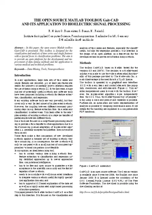
Speeding Up Multi-class SVM Evaluation by PCA and Feature Selection

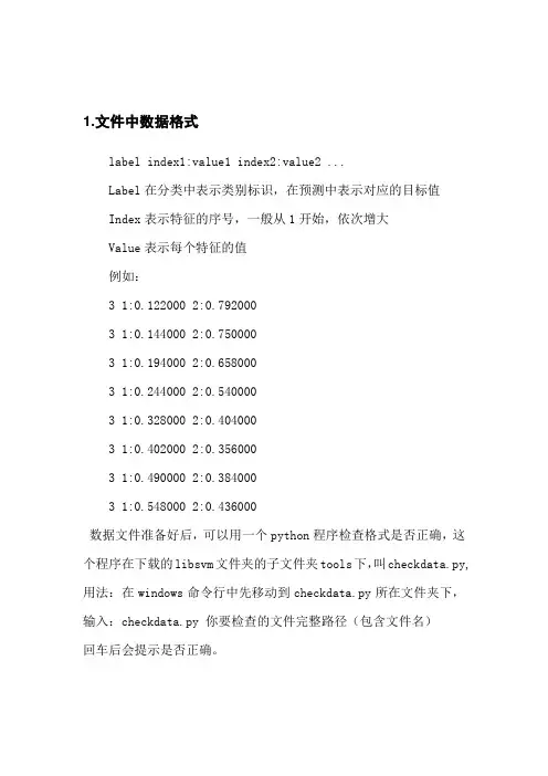
1.文件中数据格式label index1:value1 index2:value2 ...Label在分类中表示类别标识，在预测中表示对应的目标值Index表示特征的序号，一般从1开始，依次增大Value表示每个特征的值例如：3 1:0.122000 2:0.7920003 1:0.144000 2:0.7500003 1:0.194000 2:0.6580003 1:0.244000 2:0.5400003 1:0.328000 2:0.4040003 1:0.402000 2:0.3560003 1:0.490000 2:0.3840003 1:0.548000 2:0.436000数据文件准备好后，可以用一个python程序检查格式是否正确，这个程序在下载的libsvm文件夹的子文件夹tools下，叫checkdata.py,用法：在windows命令行中先移动到checkdata.py所在文件夹下，输入：checkdata.py 你要检查的文件完整路径（包含文件名）回车后会提示是否正确。

2.对数据进行归一化。

该过程要用到libsvm软件包中的svm-scale.exeSvm-scale用法：用法：svmscale [-l lower] [-u upper] [-y y_lower y_upper] [-s save_filename] [-r restore_filename] filename （缺省值： lower = -1，upper = 1，没有对y进行缩放）其中， -l：数据下限标记；lower：缩放后数据下限；-u：数据上限标记；upper：缩放后数据上限；-y：是否对目标值同时进行缩放；y_lower为下限值，y_upper 为上限值；（回归需要对目标进行缩放，因此该参数可以设定为–y -1 1 ）-s save_filename：表示将缩放的规则保存为文件save_filename；-r restore_filename：表示将缩放规则文件restore_filename载入后按此缩放；filename：待缩放的数据文件（要求满足前面所述的格式）。

支持向量机（SVM ）原理及应用一、SVM 的产生与发展自1995年Vapnik(瓦普尼克)在统计学习理论的基础上提出SVM 作为模式识别的新方法之后，SVM 一直倍受关注。

同年，Vapnik 和Cortes 提出软间隔(soft margin)SVM ，通过引进松弛变量i ξ度量数据i x 的误分类(分类出现错误时i ξ大于0)，同时在目标函数中增加一个分量用来惩罚非零松弛变量(即代价函数)，SVM 的寻优过程即是大的分隔间距和小的误差补偿之间的平衡过程；1996年，Vapnik 等人又提出支持向量回归 (Support Vector Regression ，SVR)的方法用于解决拟合问题。

SVR 同SVM 的出发点都是寻找最优超平面(注：一维空间为点；二维空间为线；三维空间为面；高维空间为超平面。

)，但SVR 的目的不是找到两种数据的分割平面，而是找到能准确预测数据分布的平面，两者最终都转换为最优化问题的求解；1998年，Weston 等人根据SVM 原理提出了用于解决多类分类的SVM 方法(Multi-Class Support Vector Machines ，Multi-SVM)，通过将多类分类转化成二类分类，将SVM 应用于多分类问题的判断：此外，在SVM 算法的基本框架下，研究者针对不同的方面提出了很多相关的改进算法。

例如，Suykens 提出的最小二乘支持向量机 (Least Square Support Vector Machine ，LS —SVM)算法，Joachims 等人提出的SVM-1ight ，张学工提出的中心支持向量机 (Central Support Vector Machine ，CSVM)，Scholkoph 和Smola 基于二次规划提出的v-SVM 等。

此后，台湾大学林智仁(Lin Chih-Jen)教授等对SVM 的典型应用进行总结，并设计开发出较为完善的SVM 工具包，也就是LIBSVM(A Library for Support Vector Machines)。

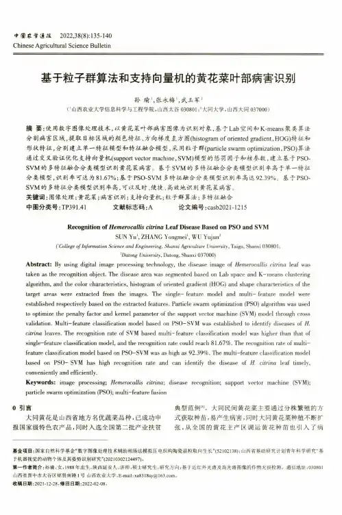
中®农f(8報 2022,38(8): 135-140Chinese Agricultural Science Bulletin基于粒子群算法和支持向量机的黄花菜叶部病害识别孙瑜'，张永梅'，武玉军2C山西农业大学信息科学与工程学院，山西太谷030801 ;2大同大学，山西大同037000)摘要:使用数字图像处理技术，以黄花菜叶部病害图像为识别对象，基于L a b空间和K-m e a n s聚类算法 分割病害区域，提取目标区域的颜色特征、方向梯度直方图(histogram of oriented gradient,H O G)特征和 形状特征，分别建立单一特征模型和特征融合模型，采用粒子群(particle swarm optimization，P S O)算法 通过交叉验证优化支持向量机(support vector machine,S V M)模型的惩罚因子和核参数，建立基于P S O-S V M的多特征融合分类模型识别黄花菜病害。

基于S V M的多特征融合分类模型识别率高于单一特征 分类模型，识别率可达为81.67%;基于P S O-S V M多特征融合分类模型识别率高达92.39%。

基于P S O-S V M的多特征分类模型识别率高，可以及时、便捷、高效地识别黄花菜病害。

关键词：图像处理；黄花菜;病害识别；支持向量机;粒子群算法；多特征融合中图分类号:T P391.41 文献标志码:A论文编号:casb2021-1215Recognition of Hemerocallis citrina Leaf Disease Based on PSO and SVMSUN Yu', ZHANG Yongmei', WU Yujun2(College of Information Science and Engineering, Shanxi Agriculture University, Taigu, Shanxi 030801;2Datong University,Datong, Shanxi 037000)Abstract：By using digital image processing technology, the disease image of H em ero ca llis c itrin a leaf was taken as the recognition object. The disease area was segmented based on Lab space and K-means clustering algorithm, and the color characteristics, histogram of oriented gradient (HOG) and shape characteristics of the target areas were extracted from the images. The single- feature model and multi- feature model were established respectively based on the extracted features. Particle swarm optimization (PSO) algorithm was used to optimize the penalty factor and kernel parameter of the support vector machine (SVM) model through cross validation. Multi-feature classification model based on PSO-SVM was established to identify diseases of H.c itrin a leaves. The recognition rate of SVM based multi-feature classification model was higher than that ofsingle-feature classification model, and the recognition rate could reach 81.67%. The recognition rate of multi­feature classification model based on PSO-SVM was as high as 92.39%. The multi-feature classification model based on PSO- SVM has high recognition rate and can identify the disease of H. c itrin a leaf timely, conveniently and efficiently.Keywords：image processing; H em ero ca llis citrin a;disease recognition; support vector machine (SVM);particle swarm optimization (PSO); multi-feature fusion0引言 典型范例[|]。

三维荧光光谱结合PCA-SVM对几种浓香型白酒的鉴别徐瑞煜;朱焯炜;胡扬俊;张毅;陈国庆【期刊名称】《光谱学与光谱分析》【年(卷),期】2016(36)4【摘要】In this paper ,a method for discrimination of different bands liquor with strong aroma type based on three‐dimensional fluorescence spectrum technology was developed .Firstly ,the three‐dimensional fluorescence spectra of seven different brands liquor were measured by the FLS920 fluorescence spectrometer which produced by Edinburgh in England .The spectral shows that different bands liquors have similar fluorescence ch aracteristics and it ’s difficult to distinguish them only with Fluorescent characteristic parameters .Because of this ,the first‐order and second‐order partial derivatives respect to fluorescenceemission wavelength on each of the excitation wavelength were carried out in this paper .Daubechies‐7 (db7) orthonormal wavelet with compact support was used to compress the spectral data .The forth approximate coefficients were finally chosen as the new data matrix .Then the new data matrix was analyzed by principal component analysis (PCA) and the principal components were ex‐tracted to be used as the inputs of support vector machine (SVM ) .The K‐fold cross validation was applied to optimize the pa‐rameters c and γand the prediction model was constructed in the end .Fourteen samples were selected randomly fromeach brand that in total of ninety‐eight samples were selected as the training set ,and the rest forty‐two samples were collected as the predic‐tion set .The effect of three different spectral data after processing on the model is compared :original data ,the first‐order and second‐order partial derivatives on the spectral data .The results show that the three‐dimensional fluorescence spectra with the pretreatment of second‐order partial derivatives coupled with PCA and SVM can make a good performance on the brands identifi‐cation of strong aroma typeliquors ,the accuracy of the established model and prediction accuracy were 98.98% and 100% ,re‐spectively .This method has the advantage of easy operation ,high speed ,low cost and provides a good help in the detection and identification of Chinese liquor .%提出一种利用三维荧光光谱技术鉴别不同品牌浓香型白酒的方法。

支持向量机的特征选取方法支持向量机（Support Vector Machine，简称SVM）是一种常用的机器学习算法，被广泛应用于分类和回归问题。

在实际应用中，选择合适的特征对于SVM的性能至关重要。

本文将介绍一些常用的支持向量机特征选取方法，帮助读者更好地理解和应用SVM算法。

一、特征选取的重要性特征选取是指从原始数据中选择出最具有代表性和区分性的特征，以提高分类或回归模型的性能。

在SVM中，特征选取的目标是找到最佳的特征子集，以提高分类超平面的判别能力和泛化能力。

二、过滤式特征选取方法过滤式特征选取方法是一种独立于具体学习算法的特征选择方法，它通过对特征进行评估和排序，然后选择排名靠前的特征子集。

常用的过滤式特征选取方法有相关系数法、卡方检验法和信息增益法等。

1. 相关系数法相关系数法是一种衡量特征与目标变量之间线性关系的方法。

它通过计算特征与目标变量之间的相关系数，选择相关性较高的特征。

在SVM中，相关系数法可以帮助我们筛选出与目标变量相关性较强的特征，提高分类模型的性能。

2. 卡方检验法卡方检验法是一种用于检验特征与目标变量之间独立性的方法。

它通过计算特征与目标变量之间的卡方值，选择卡方值较大的特征。

在SVM中，卡方检验法可以帮助我们找到与目标变量相关性较高的特征，提高分类模型的准确性。

3. 信息增益法信息增益法是一种衡量特征对于目标变量分类能力的方法。

它通过计算特征对目标变量的信息增益，选择信息增益较大的特征。

在SVM中，信息增益法可以帮助我们选择对目标变量具有较强分类能力的特征，提高分类模型的性能。

三、嵌入式特征选取方法嵌入式特征选取方法是一种将特征选取与学习算法结合起来的方法，通过学习算法自身的特性选择最佳的特征子集。

常用的嵌入式特征选取方法有L1正则化方法、决策树方法和基于遗传算法的方法等。

1. L1正则化方法L1正则化方法是一种通过在目标函数中加入L1范数惩罚项来实现特征选取的方法。

利用支持向量机进行变量重要性分析与筛选在数据分析和机器学习领域，变量重要性分析与筛选是一项关键任务。

通过确定哪些变量对于预测模型的性能和准确性具有最大的影响，我们可以优化模型并提高其预测能力。

支持向量机（Support Vector Machine，SVM）是一种强大的机器学习算法，具有广泛的应用领域。

在本文中，我们将探讨如何利用支持向量机进行变量重要性分析与筛选。

首先，让我们简要了解支持向量机的基本原理。

支持向量机是一种监督学习算法，用于分类和回归问题。

其基本思想是通过在特征空间中构建一个最优的超平面，将不同类别的数据样本分开。

支持向量机通过最大化超平面与最近的数据点之间的间隔，实现对数据的有效分类。

在变量重要性分析中，我们可以利用支持向量机的特性来评估不同变量对于分类或回归的贡献程度。

通过训练支持向量机模型，并观察每个变量对模型性能的影响，我们可以得出变量的重要性排序。

具体而言，我们可以使用以下方法来实现变量重要性分析与筛选。

首先，我们需要准备一个包含所有变量和目标变量的数据集。

接下来，我们将数据集分为训练集和测试集，以便在训练支持向量机模型时进行验证。

然后，我们使用支持向量机算法对训练集进行训练，并利用测试集评估模型的性能。

在训练过程中，支持向量机将为每个变量分配一个权重，该权重表示该变量对于模型的贡献程度。

较高的权重意味着该变量对于模型的性能具有更大的影响。

我们可以根据这些权重来确定变量的重要性，并进行筛选。

一种常用的方法是基于权重的排序。

我们可以按照变量权重的大小对变量进行排序，从而得出变量的重要性顺序。

具有较高权重的变量被认为对于模型的性能具有更大的影响，因此可以被保留下来。

相反，具有较低权重的变量可能对模型的性能影响较小，可以被剔除。

另一种方法是基于变量的影响度量。

我们可以通过计算在去除某个变量后模型性能的变化来评估该变量的重要性。

如果去除某个变量后模型性能显著下降，那么该变量被认为对于模型的性能具有重要影响，应该保留。

基于FS-PCA-MSCD的地铁轴承可视化诊断方法杨建伟;白永亮;武慧杰;化凤芳【期刊名称】《北京建筑工程学院学报》【年(卷),期】2016(032)003【摘要】针对地铁轴承的可视化故障诊断能力,本文提出了基于特征选择(Feature Selection,FS)与多尺度类距离(Multi Scale Class Distance,MSCD)的轴承故障诊断方法.首先对地铁齿轮箱轴承振动信号进行采集,获得不同故障类型的轴承故障样本集;然后基于FS方法提取故障样本中存在的敏感特征值,并利用获得的特征向量进行主成分分析(Principal Component Analysis,PCA),基于MSCD方法对各故障聚类进行再分类,提高故障类的可分性,获得可视化程度高的故障诊断结果.利用该方法对地铁齿轮箱轴承故障数据进行可视化故障诊断,诊断结果表明该方法能够提取敏感故障特征并获得具有较高故障可分性与可视化的诊断结果.该方法为地铁轴承在线故障分析能力提供了技术支持,在地铁运行维护与故障诊断方面均具有广阔的应用前景.【总页数】6页(P116-120,131)【作者】杨建伟;白永亮;武慧杰;化凤芳【作者单位】北京建筑大学机电与车辆工程学院城市轨道交通车辆服役性能保障北京市重点实验室,北京100044;北京建筑大学机电与车辆工程学院城市轨道交通车辆服役性能保障北京市重点实验室,北京100044;北京建筑大学机电与车辆工程学院城市轨道交通车辆服役性能保障北京市重点实验室,北京100044;北京建筑大学机电与车辆工程学院城市轨道交通车辆服役性能保障北京市重点实验室,北京100044【正文语种】中文【中图分类】TH17【相关文献】1.基于EMD与SVM的地铁列车滚动轴承故障诊断方法分析 [J], 彭松;黄志辉;胡奇宇2.基于FS-PCA-MSCD的地铁轴承可视化诊断方法 [J], 杨建伟;白永亮;武慧杰;化凤芳;3.基于加权改进D-S证据融合理论的地铁车辆转向架轴承故障诊断方法 [J], WANG Yuanfei;PEI Chunxing;SUN Hairong4.基于小波神经网络的地铁轴承故障诊断方法 [J], 徐欣怡;徐永能;任宇超5.基于小波神经网络的地铁轴承故障诊断方法 [J], 徐欣怡;徐永能;任宇超因版权原因，仅展示原文概要，查看原文内容请购买。