Lower limit on the mass of the neutralino (LSP) at LEP with the ALEPH detector

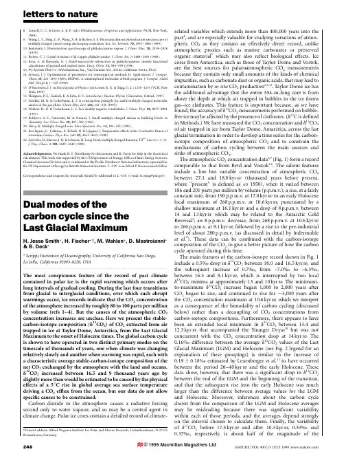
letters to nature8.Leznoff,C.C.&Lever,A.B.P.(eds)Phthalocyanines:Properties and Applications(VCH,New York,1989).9.Wang,L.S.,Ding,C.F.,Wang,X.B.&Barlow,S.E.Photodetachment photoelectron spectroscopy ofmultiply charged anions using electrospray ionization.Rev.Sci.Instrum.70,1957±1966(1999). 10.Berkowitz,J.Photoelectron spectroscopy of phthalocyanine vapors.J.Chem.Phys.70,2819±2828(1979).11.Brown,C.J.Crystal structure of b-copper phthalocyanine.J.Chem.Soc.A2488±2493(1968).12.Rosa,A.&Baerends,E.J.Metal-macrocycle interaction in phthalocyanines:density functionalcalculations of ground and excited states.Inorg.Chem.33,584±595(1994).13.PC Spartan Plus5.1(Wavefunction,Inc.,Von Carman Ave.,Irvine,California92612,USA).14.Stewart,J.J.Optimization of parameters for semiempirical methods II:put.Chem.10;221±264(1989);MOPAC:A semiempirical molecular orbital put.Aided Mol.Design4;1±105(1990).15.D'Haennens,I.J.in Encyclopedia of Physics(eds Lerner,R.G.&Trigg,G.L.)1251±1253(VCH,NewYork,1991).16.Hodgson,P.E.,Gadioli,E.&Erba,E.G.Introductory Nuclear Physics(Clarendon,Oxford,1997).17.Scheller,M.K.&Cederbaum,L.S.A construction principle for stable multiply charged molecularanions in the gas phase.Chem.Phys.Lett.216,141±146(1993).18.Weikert,H.-G.&Cederbaum,L.S.Free doubly negative tetrahalides.J.Chem.Phys.99,8877±8891(1993).19.Boldyrev,A.I.,Gutowski,M.&Simons,J.Small multiply charged anions as building blocks inchemistry.Acc.Chem.Res.29,497±502(1996).20.Vekey,K.Multiply charged ions.Mass Spectrom.Rev.14,195±225(1995).21.Brechignac,C.,Cahuzac,P.,Kebaili,N.&Leygnier,J.Temperature effects in the Coulombic®ssion ofstrontium clusters.Phys.Rev.Lett.81,4612±4615(1998).22.Schroder,D.,Harvey,J.N.&Schwarz,H.Long-lived,multiply charged diatomic TiF n+ions(n=1±3).J.Phys.Chem.A102,3639±3642(1998).Acknowledgements.We thank R.S.Disselkamp for discussions and K.Ferris for help in the theoretical calculations.This work was supported by the US Department of Energy,Of®ce of Basic Energy Sciences, Chemical Sciences Division and is conducted at the Paci®c Northwest National Laboratory,operated for the US Department of Energy by Battelle Memorial Institute.L.-S.W.is an Alfred P.Sloan research fellow.Correspondence and requests for materials should be addressed to L.-S.W.(e-mail:ls.wang@).Dual modes of thecarbon cycle since theLast Glacial MaximumH.Jesse Smith*,H.Fischer*²,M.Wahlen*,D.Mastroianni* &B.Deck**Scripps Institution of Oceanography,University of California San Diego,La Jolla,California92093-0220,USA ......................................................................................................................... The most conspicuous feature of the record of past climate contained in polar ice is the rapid warming which occurs after long intervals of gradual cooling.During the last four transitions from glacial to interglacial conditions,over which such abrupt warmings occur,ice records indicate that the CO2concentration of the atmosphere increased by roughly80to100parts per million by volume(refs1±4).But the causes of the atmospheric CO2 concentration increases are unclear.Here we present the stable-carbon-isotope composition(d13CO2)of CO2extracted from air trapped in ice at Taylor Dome,Antarctica,from the Last Glacial Maximum to the onset of Holocene times.The global carbon cycle is shown to have operated in two distinct primary modes on the timescale of thousands of years,one when climate was changing relatively slowly and another when warming was rapid,each with a characteristic average stable-carbon-isotope composition of the net CO2exchanged by the atmosphere with the land and oceans. d13CO2increased between16.5and9thousand years ago by slightly more than would be estimated to be caused by the physical effects of a58C rise in global average sea surface temperature driving a CO2ef¯ux from the ocean,but our data do not allow speci®c causes to be constrained.Carbon dioxide in the atmosphere causes a radiative forcing second only to water vapour,and so may be a central agent in climate change.Polar ice cores contain a detailed record of climate-²Present address:Alfred-Wegener-Institute for Polar and Marine Research,Columbusstrasss,D-27515 Bremerhaven,Germany.related variables which extends more than400,000years into the past4,and are especially valuable for studying variations of atmos-pheric CO2as they contain an effectively direct record,unlike atmospheric proxies such as marine carbonates or preserved organic material5which may also re¯ect biological effects.Ice cores from Antarctica,such as those of Taylor Dome and Vostok, are the best sources for palaeoatmospheric CO2measurements because they contain only small amounts of the kinds of chemical impurities,such as carbonate dust or organic acids,that may lead to contamination by in situ CO2production2,6±8.Taylor Dome ice has the additional advantage that the entire554-m-long core is from above the depth at which air trapped in bubbles in the ice forms gas±ice clathrates.This feature is important because,as we have found,the accuracy of d13CO2measurements performed on bubble-free ice may be affected by the presence of clathrates.(d13C is de®ned in Methods.)We have measured the CO2concentration and d13CO2 of air trapped in ice from Taylor Dome,Antarctica,across the last glacial termination in order to develop a time series for the carbon-isotope composition of atmospheric CO2and to constrain the mechanisms of carbon cycling between the main sources and sinks of atmospheric CO2.The atmospheric CO2concentration data3,9(Fig.1)form a record comparable to that from Byrd and Vostok1,2.The salient features include a low but variable concentration of atmospheric CO2 between27.1and18.0kyr BP(thousand years before present, where``present''is de®ned as AD1950),when it varied between 186and201parts per million by volume(p.p.m.v.);a rise,at a fairly constant rate,from190p.p.m.v.at17.0kyr BP to an early Holocene local maximum of268p.p.m.v.at10.6kyr BP,punctuated by a shallow minimum at16.1kyr BP and a drop of8p.p.m.v.between 14and13kyr BP which may be related to the Antarctic Cold Reversal3;an8p.p.m.v.decrease,from268p.p.m.v.at10.6kyr BP to260p.p.m.v.at9.1kyr BP,followed by a rise to the pre-industrial level of about280p.p.m.v.(as discussed in detail by IndermuÈhle et al.9).These data can be combined with the carbon-isotope composition of the CO2to give a better picture of how the carbon cycle operated during this time.The main features of the carbon-isotope record shown in Fig.1 include a0.5½drop in d13CO2between18.0and16.5kyr BP,and the subsequent increase of0.7½,from-7.0½to-6.3½, between16.5and9.1kyr BP,which is interrupted by two local d13CO2minima at approximately13and10kyr BP.The minimum-to-maximum d13CO2increase began1,000to2,000years after CO2began to rise,and continued to rise for,3,000years after the CO2concentration maximum at10.6kyr BP,which we interpret as a consequence of the bimodality of carbon cycling(discussed below)rather than a decoupling of CO2concentrations from carbon-isotope compositions.Furthermore,there appears to have been an extended local minimum in d13CO2between13.4and 12.3kyr BP that accompanied the Younger Dryas10but was not concurrent with the CO2concentration drop at14kyr BP.The 0.16½difference between the average d13CO2values of the Last Glacial Maximum(LGM)and Holocene(see Fig.2legend for an explanation of these groupings)is similar to the increase of 0:1960:18½estimated by Leuenberger et al.11to have occurred between the period20±40kyr BP and the early Holocene.These data show,however,that there was a signi®cant drop in d13CO2 between the end of the LGM and the beginning of the transition, and that the subsequent rise into the early Holocene was much larger than the difference between average values for the LGM and Holocene.Moreover,inferences about the carbon cycle drawn from the comparison of the LGM and Holocene averages may be misleading because there was signi®cant variability within each of those periods,and the averages depend strongly on the interval chosen to calculate them.Finally,the variability of d13CO2before17.5kyr BP and after10.3kyr BP,0.33½and 0.37½,respectively,is about half of the magnitude of theletters to natureincrease that occurs during the transition,indicating that carbon cycling also varied considerably over shorter timescales.The atmospheric portion of the carbon cycle is extremely dynamic;,20%of the CO 2in the atmosphere is exchanged with the ocean and terrestrial biosphere every year (ref.12),so the atmosphere responds very quickly to changes in CO 2cycling between these three reservoirs.The exchange of carbon can affect the isotopic composition of atmospheric CO 2for two reasons.First,the reservoirs have different carbon-isotope compositions (the d 13CO 2of the ocean is close to 0½,the terrestrial biosphere has a d 13CO 2of approximately -25½and that of pre-industrial atmos-phere was approximately -6.5½;ref.13).Second,each ¯ux of CO 2between the atmosphere and either the ocean or the terrestrial biosphere is accompanied by a different carbon-isotope fractiona-tion,resulting in isotopically unique values of d 13CO 2for each transfer.Consequently,variations in the carbon-isotope composi-tion of atmospheric CO 2can be caused by a net ¯ux of carbon between reservoirs,or by a change in the isotopic fractionation associated with a particular atmospheric ¯ux.It also follows from this that the carbon-isotope composition of the net atmospheric CO 2exchanged,d 13CO 2(ex),is a function of the relative strengths of processes which transfer CO 2into and out of the atmosphere,so different d 13CO 2(ex)values indicate different balances of processes.When a unique balance of processes persists over thousands of years,as indicated by a unique d 13CO 2(ex),we refer to it as a `mode'of the carbon cycle.In order to examine more closely the implications of the time series shown in Fig.1,it is advantageous to consider the three data groups (LGM,transition and Holocene)individually.Doing so inFig.2reveals a relationship between the concentration of atmos-pheric CO 2and its carbon-isotope composition during each of these intervals.(Figure 2is a mixing diagram,where the inverse CO 2concentration is plotted against d 13CO 2,so that addition or removal of CO 2with a given d 13C would appear as a nearly straight line with the y -intercept approximately equal to the isotopic composition of the net CO 2added to,or subtracted from,the atmosphere.)The coherent trends displayed by these groups show that the carbon cycle has operated in two distinct modes over the past 27kyr,one during the Holocene,and possibly the LGM as well,when the average d 13C of net CO 2exchanged was approximately -10½,and another during the transition,when the average d 13C of net CO 2exchanged was approximately -5½.In other words,during the period of relatively stable,slowly changing climate of the Holocene,the carbon of the net exchanged atmospheric CO 2was isotopically lighter than the average atmospheric value (that is,d d 13CO 2/dCO 2was negative).In contrast,during the period of rapidly changing climate of the transition the net exchanged CO 2was isotopically heavier (d d 13CO 2/dCO 2was positive).Therefore,these data suggest that the carbon cycle has operated in two primary modes over the past 27kyr,one when climate is changing only slowly and another when rapid warming occurs,and that although there are clearly other processes which have affected atmospheric CO 2over the past 27kyr,as is evident from the scatter in the data shown in Fig.2,those transient variations did not overwhelm the longer-term trends.Many schemes have been advanced to account for the magnitude of the rise in the concentration of atmospheric CO 2during deglaciations (see,for example,Broecker 14for a critical review),although none seem to be uniquely suf®cient.Two factors which must be included in any analysis of the glacial±interglacial increase in atmospheric CO 2content,however,are a rise in sea surface temperature (SST)and a decrease in ocean salinity (S).In the range of SST,atmospheric CO 2concentration and salinity appropriate for this study,changes in SST affect both atmospheric p CO 2and d 13CO 2,by approximately 4.2%per 8C (ref.15)and 0.11±0.13½per 8C (ref.16),respectively,while changes in salinity alter p CO 2by 10p.p.m.v.per ½S without affecting its d 13C (ref.17).Measurements per-formed on tropical corals show that SST increased by 5±68CfromFigure 1d 13CO 2and CO 2-concentration trends.The data are based on measurements of air trapped in ice from Taylor Dome,Antarctica,and are plotted against air age.Upper curve,d 13CO 2values (®lled circles)within envelopes of 1j and 2j uncertainty (indicated as dotted and solid lines,respectively;see the Methods section for details).Lower curve,CO 2concentration data shown as open circles were measured in our laboratory at SIO 3,while the solid line shown in the Holocene (for comparison)is the higher-resolution record of Indermu hle et al.9.The age axis is divided into three intervals,called ``LGM'',``transition'',and ``Holocene''on the basis of CO 2concentrations and generally accepted ages for these periods.The LGM group includes all of the points with air ages between 27.1and 18.0kyr BP ,the youngest being the last with a CO 2concentration below the highest value of the older samples.The transition group includes the points with ages between 17.0and 10.6kyr BP ,where the local CO 2maximum which we use to de®ne the start of the Holocene occurs.The Holocene group includes all the points with ages between 10.1and 1.3kyr BP (the youngest sample measured for d 13CO 2).The boundaries between the LGM and the transition,and between the transition and the Holocene,chosen here to fall at 17.5and 10.3kyr BP ,respectively,are shown as vertical dashedlines.[CO 2] (p.p.m.)1/[CO 2] (p.p.m.-1)δ13C O 2 (‰)Figure 2Mixing diagram for Taylor Dome samples:1/[CO 2]is plotted against d 13CO 2.The data are divided into three groups,as described in the ®gure:the LGM group (open triangles,6d 13CO 2points),the transition group (®lled circles,15d 13CO 2points),and the Holocene group (open squares,10d 13CO 2points).The y -intercept of the regression line through each of the three groups of data,along with the corresponding 1j uncertainty for each value,indicates the d 13C of the CO 2exchanged by the atmosphere,d 13CO 2(ex),and is shown on the ®gure.letters to naturethe last peak-glacial period to the early Holocene18,signi®cantly more than the earlier estimate of1±28C by CLIMAP19,while the change in ocean salinity,estimated from sea level change20,was approximately-1.4½.Assuming a global average D SST(sea surface temperature change)of58C,the combined effects of temperature and salinity changes should have resulted in increases in the concentration and d13CO2of roughly30p.p.m.v.and0.6½, respectively.If this were true,then all other processes which caused variations in atmospheric CO2must together have increased its concentration by,50p.p.m.v.and its d13CO2by only0.1½.A 28C global average D SST,on the other hand,would have caused no signi®cant change in the concentration of atmospheric CO2and increased d13CO2by roughly0.2½,leaving unexplained an approximately80p.p.m.concentration increase and a0.5½d13CO2increase.Adding these changes to the0.3½whole-ocean d13CO2increase which is thought to have accompanied deglaciation21,the expected increase in atmospheric d13CO2would be between0.9½and0.6½,depending on whether a D SST of5or 28C is assumed.The observed increase of0.7½would seem to imply,then,that it is not necessary to invoke a large decrease in surface ocean productivity(which would lower atmospheric d13CO2 to values more negative than are observed)to explain the d13CO2 increase during the transition.What does become necessary,then,is to explain the0.5½drop seen between18and16.5kyr BP.In the broadest sense,the atmospheric d13CO2record presented here points to the ocean as the predominant source of atmospheric CO2during the transition.This interpretation follows from two observations.First,even if a change in average global SST alone had caused the increase in d13CO2,a realistic D SST would have resulted in an increase of atmospheric CO2concentration of less than half of what is observed,so there must have been other sources of CO2 during that time.Second,because d13CO2was increasing at a rate equal to or greater than that which rising SST alone would have caused,the additional net CO2¯ux must have had a d13CO2equal to, or greater than,that of the coexisting atmosphere,eliminating the terrestrial biosphere as a possible source.The most likely explana-tion for this is an enhanced¯ux from the ocean(with a d13C close to that of the atmosphere)which transferred CO2into the atmosphere at a rate greater than the concurrent uptake of isotopically light CO2 by an expanding terrestrial biosphere.Unfortunately,the con-straints imposed by these data are insuf®cient to allow the identi-®cation of a speci®c cause for the increased¯ux of CO2from the ocean to the atmosphere.A better understanding of the carbon cycle depends not only on better models,but on additional experimental constraints on the carbon system,particularly more precise data about changes in SST,the size and composition of the terrestrial biosphere,the growth of coral reefs during periods of sea level rise, marine productivity and the chemical composition of the oceans.M ......................................................................................................................... MethodsAll samples were taken from Taylor Dome,Antarctica(7708489S,1588439E, elevation2,374m),drilled in1993/94.The methods used for determining the CO2concentration of air trapped in ice and the measurement of its carbon-isotope composition are described in detail elsewhere22,23.CO2concentration measurements have an internal precision of63p.p.m.v.(2j)and are calculated by comparison to three standards of precisely known compositions which are run with every sample.The Craig-corrected24carbon-isotope measurements, performed on our VG Prism II isotope ratio mass spectrometer,have a1j precision of60.075½,based on numerous analyses of the CO2separated from an atmospheric air standard exposed to uncrushed ice,in order to simulate the conditions of a sample run and to check for fractionation during extraction. d13CO2is reported in normal d notation as the per mil difference between the isotopic composition of the sample and standard VPDB carbon, 13C=12C sample= 13C=12C VPDB21 31;000 .The d13CO2values reported here have been corrected for the gravitational separation of gases of different masses in the®rn,and for the presence of N2O (which results in isobaric interferences with CO2during mass spectrometry).Gravitational separation in the®rn25,26was determined by using the values of d15N2of air trapped in Taylor Dome ice from Sucher27,following the approach of Sowers and Bender28.The gravitational correction for d13CO2is,0.005½per m.C-isotope data are corrected for the presence of N2O on the basis of calibrations performed in our laboratory on CO2±N2O mixtures.The N2O concentrations of atmospheric air used for this correction,adapted from Leuenberger and Siegenthaler29,are linear interpolations of the following concentrations and dates:275p.p.b.(0±9.25yr BP),200p.p.b.(16.1±27.2kyr BP).The N2O correction is,0.001½per p.p.b.of N2O.The total1j uncertainty in the reported d13CO2of a single sample,including uncertainties in the gravitational and N2O corrections,is0.085½.Duplicate analyses of samples with air ages of2.19and17.2kyr BP have a1j uncertainty of0.060½and a triplicate analysis of the sample with an air age of27.4kyr BP has a1j uncertainty of0.049½.The depth±age scale and air age±ice age differences were calculated using a combination of¯ow modelling,correlating variations in the d18O of the ice with the well-dated GISP2,and matching atmospheric CH4concentrations and d18O of O2with variations seen in GISP230.Received8October1998;accepted7June1999.1.Barnola,J.M.,Raynaud,D.,Korotkevich,Y.S.&Lorius,C.Vostok ice core provides160,000-yearrecord of atmospheric CO2.Nature329,408±414(1987).2.Neftel,A.,Oeschger,H.,Staffelbach,T.&Stauffer,B.CO2record in the Byrd ice core50,000±5,000years BP.Nature331,609±611(1988).3.Fischer,H.,Wahlen,M.,Smith,H.J.,Mastroianni,D.&Deck,B.Ice core records of atmospheric CO2around the last three glacial terminations.Science283,1712±1714(1999).4.Petit,J.R.et al.Climate and atmospheric history of the past420,000years from the Vostok ice core,Antarctica.Nature399,429±436(1999).5.Marino,B.,McElroy,M.B.,Salawitch,R.J.&Spaulding,W.G.Glacial-to-interglacial variations in thecarbon isotopic composition of atmospheric CO2.Nature357,461±466(1992).6.Anklin,M.,Barnola,J.-M.,Schwander,J.,Stauffer,B.&Raynaud,D.Processes affecting the CO2concentrations measured in Greenland ice.Tellus B47,461±470(1995).7.Delmas,R.J.A natural artefact in Greenland ice core CO2measurements.Tellus B45,391±396(1993).8.Barnola,J.M.et al.CO2evolution during the last millennium as recorded by Antarctic and Greenlandice.Tellus B47,264±272(1995).9.IndermuÈhle,A.et al.Holocene carbon-cycle dynamics based on CO2trapped in ice at Taylor Dome,Antarctica.Nature398,121±126(1999).10.Fairbanks,R.G.The age and origin of the``Younger Dryas Climate Event''in Greenland ice cores.Paleoceanography5,937±948(1990).11.Leuenberger,M.,Siegenthaler,U.&Langway,C.C.Carbon isotope composition of atmospheric CO2during the last ice age from an Antarctic ice core.Nature357,488±490(1992).12.Tans,P.P.,Berry,J.A.&Keeling,R.F.Oceanic13C/12C observations:a new window on ocean CO2uptake.Glob.Biogeochem.Cycles7,353±368(1993).13.Friedli,H.,Lotscher,H.,Oeschger,H.,Siegenthaler,U.&Stauffer,B.Ice core record of the13C/12C ofatmospheric CO2in the past two centuries.Nature324,237±238(1986).14.Broecker,W.S.&Henderson,G.M.The sequence of events surrounding T ermination II and theirimplications for the cause of glacial-interglacial CO2changes.Paleoceanography13,352±364(1998).15.Takahashi,T.,Olafsson,J.,Goddard,J.G.,Chipman,D.W.&Sutherland,S.C.Seasonal variation ofCO2and nutrients in the high-latitude surface oceans:a comparative study.Glob.Biogeochem.Cycles 7,843±878(1993).16.Mook,W.G.,Bommerson,J.C.&Staverman,W.H.Carbon isotope fractionation between dissolvedbicarbonate and gaseous carbon dioxide.Earth Planet.Sci.Lett.22,169±176(1974).17.Weiss,R.F.Carbon dioxide in water and seawater:the solubility of a non-ideal gas.Mar.Chem.2,203±215(1974).18.Guilderson,T.P.,Fairbanks,R.G.&Rubenstone,J.L.Tropical temperature variations since20,000years ago:modulating interhemispheric climate change.Science263,663±665(1994).19.CLIMAP Project Members Seasonal Reconstructions of the Earth's Surface at the Last Glacial Maximum(Map and Chart Ser.,MC-36,Geol.Soc.Am.,Boulder,1981).20.Fairbanks,R.G.A17,000-year glacio-eustatic sea level recordÐin¯uence of glacial melting rates onthe Younger Dryas Event and deep-ocean circulation.Nature342,637±642(1989).21.Duplessy,J.C.et al.Deepwater source variations during the last climatic cycle and their impact on theglobal deepwater circulation.Paleoceanography3,343±360(1988).22.Wahlen,M.,Allen,D.&Deck,B.Initial measurements of CO2concentrations(1530to1940AD)in airoccluded in the GISP2ice core from central Greenland.Geophys.Res.Lett.18,1457±1460(1991).23.Smith,H.J.,Wahlen,M.,Mastroianni,D.&Taylor,K.C.The CO2concentration of air trapped inGISP2ice from the LGM-Holocene transition.Geophys.Res.Lett.24,1±4(1997).24.Craig,H.Isotopic standards for carbon and oxygen and correction factors for mass-spectrometricanalysis of carbon dioxide.Geochim.Cosmochim.Acta12,133±149(1957).25.Craig,H.,Horibe,Y.&Sowers,T.Gravitational separation of gases and isotopes in polar ice caps.Science242,1675±1678(1988).26.Schwander,J.The Environmental Record in Glaciers and Ice Sheets(eds Oeschger,H.and Langway,C.C.)53±67(Wiley and Sons,New York,1989).27.Sucher,C.Trapped Gases in the Taylor Dome Ice Core:Implications for East Antarctic Climate Change.Thesis,Univ.Rhode Island(1997).28.Sowers,T.&Bender,M.Elemental and isotopic composition of occluded O2and N2in polar ice.J.Geophys.Res.94,5137±5150(1989).29.Leuenberger,M.&Siegenthaler,U.Ice-age atmospheric concentration of nitrous oxide from anAntarctic ice core.Nature360,449±451(1988).30.Steig,E.J.et al.Synchronous climate changes in Antarctica and the North Atlantic.Science282,92±95(1998).Acknowledgements.We thank G.Hargreaves and J.Fitzpatrick for help obtaining samples,and E.Steig and E.Brook for sharing their depth-age scales.This work was supported by the NSF and the Director's of®ce at the Scripps Institution of Oceanography.Correspondence and requests for materials should be addressed to H.J.S.(e-mail:hjsmith@).。

a r X i v :h e p -e x /0207007v 1 1 J u l 2002BELLEBelle Prerpint 2002-18KEK Preprint 2002-59Study of B →ρπdecays at BelleBelle Collaboration A.Gordon u ,Y.Chao z ,K.Abe h ,K.Abe aq ,N.Abe at ,R.Abe ac ,T.Abe ar ,Byoung Sup Ahn o ,H.Aihara as ,M.Akatsu v ,Y.Asano ay ,T.Aso aw ,V.Aulchenko b ,T.Aushev ℓ,A.M.Bakich an ,Y.Ban ag ,A.Bay r ,I.Bedny b ,P.K.Behera az ,jak m ,A.Bondar b ,A.Bozek aa ,M.Braˇc ko t ,m ,T.E.Browder g ,B.C.K.Casey g ,M.-C.Chang z ,P.Chang z ,B.G.Cheon am ,R.Chistov ℓ,Y.Choi am ,Y.K.Choi am ,M.Danilov ℓ,L.Y.Dong j ,J.Dragic u ,A.Drutskoy ℓ,S.Eidelman b ,V.Eiges ℓ,Y.Enari v ,C.W.Everton u ,F.Fang g ,H.Fujii h ,C.Fukunaga au ,N.Gabyshev h ,A.Garmash b ,h ,T.Gershon h ,B.Golob s ,m ,R.Guo x ,J.Haba h ,T.Hara ae ,Y.Harada ac ,N.C.Hastings u ,H.Hayashii w ,M.Hazumi h ,E.M.Heenan u ,I.Higuchi ar ,T.Higuchi as ,L.Hinz r ,T.Hokuue v ,Y.Hoshi aq ,S.R.Hou z ,W.-S.Hou z ,S.-C.Hsu z ,H.-C.Huang z ,T.Igaki v ,Y.Igarashi h ,T.Iijima v ,K.Inami v ,A.Ishikawa v ,H.Ishino at ,R.Itoh h ,H.Iwasaki h ,Y.Iwasaki h ,H.K.Jang a ℓ,J.H.Kang bc ,J.S.Kang o ,N.Katayama h ,Y.Kawakami v ,N.Kawamura a ,T.Kawasaki ac ,H.Kichimi h ,D.W.Kim am ,Heejong Kim bc ,H.J.Kim bc ,H.O.Kim am ,Hyunwoo Kim o ,S.K.Kim a ℓ,T.H.Kim bc ,K.Kinoshita e ,S.Korpar t ,m ,P.Krokovny b ,R.Kulasiri e ,S.Kumar af ,A.Kuzmin b ,Y.-J.Kwon bc ,nge f ,ai ,G.Leder k ,S.H.Lee a ℓ,J.Li ak ,A.Limosani u ,D.Liventsevℓ,R.-S.Lu z,J.MacNaughton k,G.Majumder ao, F.Mandl k,D.Marlow ah,S.Matsumoto d,T.Matsumoto au,W.Mitaroffk,K.Miyabayashi w,Y.Miyabayashi v,H.Miyake ae,H.Miyata ac,G.R.Moloney u,T.Mori d,T.Nagamine ar,Y.Nagasaka i,T.Nakadaira as,E.Nakano ad, M.Nakao h,J.W.Nam am,Z.Natkaniec aa,K.Neichi aq, S.Nishida p,O.Nitoh av,S.Noguchi w,T.Nozaki h,S.Ogawa ap, T.Ohshima v,T.Okabe v,S.Okuno n,S.L.Olsen g,Y.Onuki ac, W.Ostrowicz aa,H.Ozaki h,P.Pakhlovℓ,H.Palka aa,C.W.Park o,H.Park q,L.S.Peak an,J.-P.Perroud r, M.Peters g,L.E.Piilonen ba,J.L.Rodriguez g,F.J.Ronga r, N.Root b,M.Rozanska aa,K.Rybicki aa,H.Sagawa h,S.Saitoh h,Y.Sakai h,M.Satapathy az,A.Satpathy h,e,O.Schneider r,S.Schrenk e,C.Schwanda h,k,S.Semenovℓ,K.Senyo v,R.Seuster g,M.E.Sevior u,H.Shibuya ap,V.Sidorov b,J.B.Singh af,S.Staniˇc ay,1,M.Stariˇc m,A.Sugi v, A.Sugiyama v,K.Sumisawa h,T.Sumiyoshi au,K.Suzuki h,S.Suzuki bb,S.Y.Suzuki h,T.Takahashi ad,F.Takasaki h, K.Tamai h,N.Tamura ac,J.Tanaka as,M.Tanaka h,G.N.Taylor u,Y.Teramoto ad,S.Tokuda v,S.N.Tovey u,T.Tsuboyama h,T.Tsukamoto h,S.Uehara h,K.Ueno z, Y.Unno c,S.Uno h,hiroda h,G.Varner g,K.E.Varvell an,C.C.Wang z,C.H.Wang y,J.G.Wang ba,M.-Z.Wang z,Y.Watanabe at,E.Won o,B.D.Yabsley ba,Y.Yamada h, A.Yamaguchi ar,Y.Yamashita ab,M.Yamauchi h,H.Yanai ac,P.Yeh z,Y.Yuan j,Y.Yusa ar,J.Zhang ay,Z.P.Zhang ak,Y.Zheng g,and D.ˇZontar aya Aomori University,Aomori,Japanb Budker Institute of Nuclear Physics,Novosibirsk,Russiac Chiba University,Chiba,Japand Chuo University,Tokyo,Japane University of Cincinnati,Cincinnati,OH,USAf University of Frankfurt,Frankfurt,Germanyg University of Hawaii,Honolulu,HI,USAh High Energy Accelerator Research Organization(KEK),Tsukuba,Japani Hiroshima Institute of Technology,Hiroshima,Japanj Institute of High Energy Physics,Chinese Academy of Sciences,Beijing,PRChinak Institute of High Energy Physics,Vienna,Austria ℓInstitute for Theoretical and Experimental Physics,Moscow,Russiam J.Stefan Institute,Ljubljana,Slovenian Kanagawa University,Yokohama,Japano Korea University,Seoul,South Koreap Kyoto University,Kyoto,Japanq Kyungpook National University,Taegu,South Korear Institut de Physique des Hautes´Energies,Universit´e de Lausanne,Lausanne,Switzerlands University of Ljubljana,Ljubljana,Sloveniat University of Maribor,Maribor,Sloveniau University of Melbourne,Victoria,Australiav Nagoya University,Nagoya,Japanw Nara Women’s University,Nara,Japanx National Kaohsiung Normal University,Kaohsiung,Taiwany National Lien-Ho Institute of Technology,Miao Li,Taiwanz National Taiwan University,Taipei,Taiwanaa H.Niewodniczanski Institute of Nuclear Physics,Krakow,Polandab Nihon Dental College,Niigata,Japanac Niigata University,Niigata,Japanad Osaka City University,Osaka,Japanae Osaka University,Osaka,Japanaf Panjab University,Chandigarh,Indiaag Peking University,Beijing,PR Chinaah Princeton University,Princeton,NJ,USAai RIKEN BNL Research Center,Brookhaven,NY,USAaj Saga University,Saga,Japanak University of Science and Technology of China,Hefei,PR ChinaaℓSeoul National University,Seoul,South Koreaam Sungkyunkwan University,Suwon,South Koreaan University of Sydney,Sydney,NSW,Australiaao Tata Institute of Fundamental Research,Bombay,Indiaap Toho University,Funabashi,Japanaq Tohoku Gakuin University,Tagajo,Japanar Tohoku University,Sendai,Japanas University of Tokyo,Tokyo,Japanat Tokyo Institute of Technology,Tokyo,Japanau Tokyo Metropolitan University,Tokyo,Japanav Tokyo University of Agriculture and Technology,Tokyo,Japanaw Toyama National College of Maritime Technology,Toyama,Japanay University of Tsukuba,Tsukuba,Japanaz Utkal University,Bhubaneswer,Indiaba Virginia Polytechnic Institute and State University,Blacksburg,VA,USAbb Yokkaichi University,Yokkaichi,Japanbc Yonsei University,Seoul,South KoreaB events collected with the Belle detector at KEKB.Thebranching fractions B(B+→ρ0π+)=(8.0+2.3+0.7−2.0−0.7)×10−6and B(B0→ρ±π∓)=(20.8+6.0+2.8−6.3−3.1)×10−6are obtained.In addition,a90%confidence level upper limitof B(B0→ρ0π0)<5.3×10−6is reported.Key words:ρπ,branching fractionPACS:13.25.hw,14.40.Nd1on leave from Nova Gorica Polytechnic,Nova Gorica,Sloveniamodes are examined.Here and throughout the text,inclusion of charge con-jugate modes is implied and for the neutral decay,B0→ρ±π∓,the notation implies a sum over both the modes.The data sample used in this analysis was taken by the Belle detector[9]at KEKB[10],an asymmetric storage ring that collides8GeV electrons against3.5GeV positrons.This produces Υ(4S)mesons that decay into B0B pairs.The Belle detector is a general purpose spectrometer based on a1.5T su-perconducting solenoid magnet.Charged particle tracking is achieved with a three-layer double-sided silicon vertex detector(SVD)surrounded by a central drift chamber(CDC)that consists of50layers segmented into6axial and5 stereo super-layers.The CDC covers the polar angle range between17◦and 150◦in the laboratory frame,which corresponds to92%of the full centre of mass(CM)frame solid angle.Together with the SVD,a transverse momen-tum resolution of(σp t/p t)2=(0.0019p t)2+(0.0030)2is achieved,where p t is in GeV/c.Charged hadron identification is provided by a combination of three devices: a system of1188aerogelˇCerenkov counters(ACC)covering the momentum range1–3.5GeV/c,a time-of-flight scintillation counter system(TOF)for track momenta below1.5GeV/c,and dE/dx information from the CDC for particles with very low or high rmation from these three devices is combined to give the likelihood of a particle being a kaon,L K,or pion, Lπ.Kaon-pion separation is then accomplished based on the likelihood ratio Lπ/(Lπ+L K).Particles with a likelihood ratio greater than0.6are identified as pions.The pion identification efficiencies are measured using a high momentum D∗+data sample,where D∗+→D0π+and D0→K−π+.With this pion selection criterion,the typical efficiency for identifying pions in the momentum region0.5GeV/c<p<4GeV/c is(88.5±0.1)%.By comparing the D∗+data sample with a Monte Carlo(MC)sample,the systematic error in the particle identification(PID)is estimated to be1.4%for the mode with three charged tracks and0.9%for the modes with two.Surrounding the charged PID devices is an electromagnetic calorimeter(ECL) consisting of8736CsI(Tl)crystals with a typical cross-section of5.5×5.5cm2 at the front surface and16.2X0in depth.The ECL provides a photon energy resolution of(σE/E)2=0.0132+(0.0007/E)2+(0.008/E1/4)2,where E is in GeV.Electron identification is achieved by using a combination of dE/dx measure-ments in the CDC,the response of the ACC and the position and shape of the electromagnetic shower from the ECL.Further information is obtained from the ratio of the total energy registered in the calorimeter to the particle momentum,E/p lab.Charged tracks are required to come from the interaction point and have transverse momenta above100MeV/c.Tracks consistent with being an elec-tron are rejected and the remaining tracks must satisfy the pion identification requirement.The performance of the charged track reconstruction is studied using high momentumη→γγandη→π+π−π0decays.Based on the relative yields between data and MC,we assign a systematic error of2%to the single track reconstruction efficiency.Neutral pion candidates are detected with the ECL via their decayπ0→γγ. Theπ0mass resolution,which is asymmetric and varies slowly with theπ0 energy,averages toσ=4.9MeV/c2.The neutral pion candidates are selected fromγγpairs by requiring that their invariant mass to be within3σof the nominalπ0mass.To reduce combinatorial background,a selection criteria is applied to the pho-ton energies and theπ0momenta.Photons in the barrel region are required to have energies over50MeV,while a100MeV requirement is made for photons in the end-cap region.Theπ0candidates are required to have a momentum greater than200MeV/c in the laboratory frame.Forπ0s from BE2beam−p2B and the energy difference∆E=E B−E beam.Here, p B and E B are the momentum and energy of a B candidate in the CM frame and E beam is the CM beam energy.An incorrect mass hypothesis for a pion or kaon produces a shift of about46MeV in∆E,providing extra discrimination between these particles.The width of the M bc distributions is primarily due to the beam energy spread and is well modelled with a Gaussian of width 3.3MeV/c2for the modes with a neutral pion and2.7MeV/c2for the mode without.The∆E distribution is found to be asymmetric with a small tail on the lower side for the modes with aπ0.This is due toγinteractions withmaterial in front of the calorimeter and shower leakage out of the calorimeter. The∆E distribution can be well modelled with a Gaussian when no neutral particles are present.Events with5.2GeV/c2<M bc<5.3GeV/c2and|∆E|< 0.3GeV are selected for thefinal analysis.The dominant background comes from continuum e+e−→qB events and jet-like qi,j|p i||p j|P l(cosθij)i,k|p i||p k|,r l=),where L s and L qqD0π+ decays.By comparing the yields in data and MC after the likelihood ratiorequirement,the systematic errors are determined to be4%for the modes with aπ0and6%for the mode without.Thefinal variable used for continuum suppression is theρhelicity angle,θh, defined as the angle between the direction of the decay pion from theρin the ρrest frame and theρin the B rest frame.The requirement of|cosθh|>0.3 is made independently of the likelihood ratio as it is effective in suppressing the background from B decays as well as the qB events is used[14].The largest component of this background is found to come from decays of the type B→Dπ;when the D meson decays via D→π+π−,events can directly reach the signal region while the decay D→K−π+can reach the signal region with the kaon misidentified as a pion.Decays with J/ψandψ(2S) mesons can also populate the signal region if both the daughter leptons are misidentified as pions.These events are excluded by making requirements on the invariant mass of the intermediate particles:|M(π+π−)−M D0|>0.14 GeV/c2,|M(π+π0)−M D+|>0.05GeV/c2,|M(π+π−)−M J/ψ|>0.07GeV/c2 and|M(π+π−)−Mψ(2S)|>0.05GeV/c2.The widest cut is made around the D0mass to account for the mass shift due to misidentifying the kaons in D0 decays as pions.Fig.1shows the∆E and M bc distributions for the three modes analysed after all the selection criteria have been applied.The∆E and M bc plots are shown for events that lie within3σof the nominal M bc and∆E values,respectively. The signal yields are obtained by performing maximum likelihoodfits,each using a single signal function and one or more background functions.The signal functions are obtained from the MC and adjusted based on comparisons of B+→B0are assumed to be equal.The M bc distribution for all modes isfitted with a single Gaussian and an ARGUS background function[15].The normalization of the ARGUS function is left tofloat and shape of the function isfixed from the∆E sideband:−0.25 GeV<∆E<−0.08GeV and5.2GeV/c2<M bc<5.3GeV/c2.For the mode with only charged pions in thefinal state,the∆E distribution isfitted with a single Gaussian for the signal and a linear function withfixed shape for the continuum background.The normalization of the linear function is left to float and the slope isfixed from the M bc sideband,5.2GeV/c2<M bc<5.26GeV/c2,|∆E|<0.3GeV.There are also other rare B decays that are expected to contaminate the∆E distribution.For the mode without aπ0,these modes are of the type B0→h+h−(where h denotes aπor K),B→ρρ(including all combinations of charged and neutralρmesons,where the polarizations of theρmesons are assumed to be longitudinal)and B→Kππ(including the decays B+→ρ0K+,B+→K∗0π+,B+→K∗0(1430)0π+,B+→f0(980)K+ and B+→f0(1370)K+)[16].These background modes are accounted for by using smoothed histograms whose shapes have been determined by combining MC distributions.The three B→ρρmodes are combined into one histogram. The normalization of this component is allowed tofloat in thefit due to the uncertainty in the branching fractions of the B→ρρmodes.Likewise,the B→hh and all the B→Kππmodes are combined to form one hh and one Kππcomponent.The normalizations of these components arefixed to their expected yields,which are calculated using efficiencies determined by MC and branching fractions measured by previous Belle analyses[16,17].The∆Efits for the modes with aπ0in thefinal state have the signal compo-nent modelled by a Crystal Ball function[18]to account for the asymmetry in the∆E distribution.As for the B+→ρ0π+mode,the continuum background is modelled by a linear function withfixed slope.Unlike the B+→ρ0π+mode, a component is included for the background from the b→c transition.The pa-rameterization for rare B decays includes one component for the B→Kππ0 modes(B0→ρ+K−and B0→K∗+π−)[19]and one for all the B→ρρmodes.The normalization of the B→ρρcomponent is left tofloat while the other components from B decays arefixed to their expected yields.Table1summarizes the results of the∆Efits,showing the number of events, signal yields,reconstruction efficiencies,statistical significance and branching fractions or upper limits for eachfit.The statistical significance is defined assystematic error in thefitted signal yield is estimated by independently varying eachfixed parameter in thefit by1σ.Thefinal results are B(B+→ρ0π+)=(8.0+2.3+0.7−2.0−0.7)×10−6and B(B0→ρ±π∓)=(20.8+6.0+2.8−6.3−3.1)×10−6where thefirst error is statistical and the second is systematic.For theρ0π0mode,one standard deviation of the systematic error is added to the statistical limit to obtain a conservative upper limit at90%confidence of5.3×10−6.The possibility of a nonresonant B→πππbackground is also examined.To check for this type of background,the M bc and∆E yields are determined for differentππinvariant mass bins.Byfitting the M bc distribution inππinvariant mass bins with B→ρπand B→πππMC distributions,the nonresonant contribution is found to be below4%.To account for this possible background, errors3.7%and3.2%are added in quadrature to the systematic errors of the ρ+π−andρ0π+modes,respectively.Theππinvariant mass distributions are shown in Fig.2.Two plots are shown for theρ+π−andρ0π+modes,one with events from the M bc sideband superimposed over the events from the signal region(upper)and one with events from signal MC superimposed over events from the signal region with the sideband subtracted(lower).Fig.3 shows the distribution of the helicity variable,cosθh,for the two modes with all selection criteria applied except the helicity condition.Events fromρπdecays are expected to follow a cos2θdistribution while nonresonant and other background decays have an approximately uniform distribution.The helicity plots are obtained byfitting the M bc distribution in eight helicity bins ranging from−1to1.The M bc yield is then plotted against the helicity bin for each mode and the expected MC signal distributions are superimposed.Both the ππmass spectrum and the helicity distributions provide evidence that the signal events are consistent with being fromρπdecays.The results obtained here can be used to calculate the ratio of branching frac-tions R=B(B0→ρ±π∓)/B(B+→ρ0π+),which gives R=2.6±1.0±0.4, where thefirst error is statistical and second is systematic.This is consistent with values obtained by CLEO[20]and BaBar[21,22]as shown in Table2. Theoretical calculations done at tree level assuming the factorization approx-imation for the hadronic matrix elements give R∼6[3].Calculations that include penguin contributions,off-shell B∗excited states or additionalππres-onances[4–8]might yield better agreement with the the measured value of R.In conclusion,statistically significant signals have been observed in the B→ρπmodes using a31.9×106BWe wish to thank the KEKB accelerator group for the excellent operation of the KEKB accelerator.We acknowledge support from the Ministry of Ed-ucation,Culture,Sports,Science,and Technology of Japan and the Japan Society for the Promotion of Science;the Australian Research Council and the Australian Department of Industry,Science and Resources;the National Science Foundation of China under contract No.10175071;the Department of Science and Technology of India;the BK21program of the Ministry of Education of Korea and the CHEP SRC program of the Korea Science and Engineering Foundation;the Polish State Committee for Scientific Research under contract No.2P03B17017;the Ministry of Science and Technology of the Russian Federation;the Ministry of Education,Science and Sport of the Republic of Slovenia;the National Science Council and the Ministry of Education of Taiwan;and the U.S.Department of Energy.References[1] A.E.Snyder and H.R.Quinn,Phys.Rev.D48,2139(1993).[2]I.Bediaga,R.E.Blanco,C.G¨o bel,and R.M´e ndez-Galain,Phys.Rev.Lett.81,4067(1998).[3]M.Bauer,B.Stech,and M.Wirbel,Z.Phys.C34,103(1987).[4] A.Deandrea et al.,Phys.Rev.D62,036001(2000).[5]Y.H.Chen,H.Y.Cheng,B.Tseng and K.C.Yang,Phys.Rev.D60,094014(1999).[6] C.D.Lu and M.Z.Yang,Eur.Phys.J C23,275(2002).[7]J.Tandean and S.Gardner,SLAC-PUB-9199;hep-ph/0204147.[8]S.Gardner and Ulf-G.Meißner,Phys.Rev.D65,094004(2002).[9]Belle Collaboration,A.Abashian et al.,Nucl.Instr.and Meth.A479,117(2002).[10]E.Kikutani ed.,KEK Preprint2001-157(2001),to appear in Nucl.Instr.andMeth.A.[11]G.C.Fox and S.Wolfram,Phys.Rev.Lett.41,1581(1978).[12]This modification of the Fox-Wolfram moments wasfirst proposed in a seriesof lectures on continuum suppression at KEK by Dr.R.Enomoto in May and June of1999.For a more detailed description see Belle Collaboration,K.Abe et al.,Phys.Lett.B511,151(2001).[13]CLEO Collaboration,D.M.Asner et al.,Phys.Rev.D53,1039(1996).[14]These MC events are generated with the CLEO group’s QQ program,see/public/CLEO/soft/QQ.The detector response is simulated using GEANT,R.Brun et al.,GEANT 3.21,CERN Report DD/EE/84-1,1984.[15]The ARGUS Collaboration,H.Albrecht et al.,Phys.Lett.B241,278(1990).[16]Belle Collaboration,A.Garmash et al.,Phys.Rev.D65,092005(2002).[17]Belle Collaboration,K.Abe et al.,Phys.Rev.Lett.87,101801(2001).[18]J.E.Gaiser et al.,Phys.Rev.D34,711(1986).[19]Belle Collaboration,K.Abe et al.,BELLE-CONF-0115,submitted as acontribution paper to the2001International Europhysics Conference on High Energy Physics(EPS-HEP2001).[20]CLEO Collaboration,C.P.Jessop et al.,Phys.Rev.Lett.85,2881(2000).[21]Babar Collaboration,B.Aubert et al.,submitted as a contribution paper tothe20th International Symposium on Lepton and Photon Interactions at High Energy(LP01);hep-ex/0107058.[22]BaBar Collaboration,B.Aubert et al.,submitted as a contribution paper tothe XXXth International Conference on High Energy Physics(ICHEP2000);hep-ex/0008058.Table1∆Efit results.Shown for each mode are the number of events in thefit,the signal yield,the reconstruction efficiency,the branching fraction(B)or90%confidence level upper limit(UL)and the statistical significance of thefit.Thefirst error in the branching fraction is statistical,the second is systematic.ρ0π+15424.3+6.9−6.29.68.0+2.3+0.7−2.0−0.74.4σρ+π−30144.6+12.8−13.46.820.8+6.0+2.8−6.3−3.13.7σρ0π0116−4.4±8.58.5<5.3-Experiment B(B0→ρ±π∓)×10−6B(B+→ρ0π+)×10−6RE v e n t s /16 M e VE v e n t s /3 M e V /c2(b) ρ0π+Signal backgrd02.557.51012.51517.52022.55.25.225 5.25 5.2755.3E v e n t s /18 M e VE v e n t s /2 M e V /c2(d) ρ+π-Signal backgrd051015202530355.25.225 5.25 5.2755.3∆E(GeV)E v e n t s /18 M e V(e) ρ0π024681012-0.2-0.10.10.2(GeV/c 2)E v e n t s /2 M e V /c2M bc (f) ρ0πSignal backgrd02468101214165.25.225 5.25 5.2755.3Fig.1.The ∆E (left)and M bc (right)fits to the three B →ρπmodes:ρ0π+,ρ+π−and ρ0π0.The histograms show the data,the solid lines show the total fit and the dashed lines show the continuum component.In (a)the contribution from the B →ρρand B →hh modes is shown by the cross hatched component.In (c)the cross hatched component shows the contribution from the b →c transition and B →ρρmodes.102030405060+0(GeV/c 2)E v e n t s /0.1 G e V /c2M(π+π0)(GeV/c 2)E v e n t s /0.1 G e V /c2(GeV/c 2)E v e n t s /0.1 G e V /c2+-(GeV/c 2)E v e n t s /0.1 G e V /c2M(π+ π-)510152025Fig.2.The M (ππ)distributions for B 0→ρ±π∓(left)and B +→ρ0π+(right)events in the signal region.Plots (a)and (b)show sideband events superimposed;plots (c)and (d)show the sideband subtracted plots with signal MC superimposed.-1-0.500.51M b c y i e l d (E v e n t s )cos θh-1-0.500.51M b c y i e l d (E v e n t s )cos θhFig.3.The ρmeson helicity distributions for B 0→ρ±π∓(a)and B +→ρ0π+(b).Signal MC distributions are shown superimposed.。

２０２１年第４７卷第６期无线电通信技术

６７９　

ｄｏｉ：１０．３９６９／ｊ．ｉｓｓｎ．１００３－３１１４．２０２１．０６．００２引用格式：赵亚军，菅梦楠．６Ｇ智能超表面技术应用与挑战［Ｊ］．无线电通信技术，２０２１，４７（６）：６７９－６９１．［ＺＨＡＯＹａｊｕｎ，ＪＩＡＮＭｅｎｇｎａｎ．ＡｐｐｌｉｃａｔｉｏｎｓａｎｄＣｈａｌｌｅｎｇｅｓｏｆＲｅｃｏｎｆｉｇｕｒａｂｌｅＩｎｔｅｌｌｉｇｅｎｔＳｕｒｆａｃｅｆｏｒ６ＧＮｅｔｗｏｒｋｓ［Ｊ］．ＲａｄｉｏＣｏｍｍｕｎｉ⁃

ｃａｔｉｏｎｓＴｅｃｈｎｏｌｏｇｙ，２０２１，４７（６）：６７９－６９１．］

６Ｇ智能超表面技术应用与挑战

赵亚军１，２，菅梦楠１，２（１．中兴通讯股份有限公司，北京１００１９２；２．移动网络和移动多媒体技术国家重点实验室，广东深圳５１８０５５）

摘　要：智能超表面（ＲｅｃｏｎｆｉｇｕｒａｂｌｅＩｎｔｅｌｌｉｇｅｎｔＳｕｒｆａｃｅ，ＲＩＳ）因为其能够灵活操控信道环境中的电磁特性，在学术研究及产业推进上发展迅速，被认为是５Ｇ⁃Ａｄｖａｎｃｅｄ和６Ｇ网络的关键候选技术之一。ＲＩＳ通过其人为灵活异常调控无线电波传输的能力，有机会构建一个智能的无线电磁环境。ＲＩＳ的引入可能构建全新的网络范式，在给未来网络带来全新可能的同时，也导致了诸多全新的技术及工程应用挑战。该综述首先从新的角度介绍了ＲＩＳ使能未来无线通信网络的主要方面，然后重点对ＲＩＳ引入后面临的关键挑战进行了探讨。归纳汇总了ＲＩＳ网络面临的主要工程化应用技术挑战，并对其中信道降秩、网络间共存、网络内共存、网络部署等几方面的关键技术挑战进行了深入分析和探讨，提出可能的解决方案。关键词：６Ｇ；智能超表面；信道降秩；多网络共存；多用户复用；多小区共存；网络部署

中图分类号：ＴＮ９２９．５ 文献标志码：Ａ 开放科学（资源服务）标识码（ＯＳＩＤ）：文章编号：１００３－３１１４（２０２１）０６－０６７９－１３ＡｐｐｌｉｃａｔｉｏｎｓａｎｄＣｈａｌｌｅｎｇｅｓｏｆＲｅｃｏｎｆｉｇｕｒａｂｌｅＩｎｔｅｌｌｉｇｅｎｔ

AXIONSGEORG RAFFELTMax-Planck-Institut für Physik(Werner-Heisenberg-Institut),Föhringer Ring6,80805München,Germany(e-mail:*****************.de)(Received7August2001;accepted29August2001)Abstract.Axions are one of the few particle-physics candidates for dark matter which are well motivated independently of their possible cosmological role.A brief review is given of the theoreticalmotivation for axions,their possible role in cosmology,the existing astrophysical limits,and thestatus of experimental searches.1.IntroductionDespite its uncanny success,the particle-physics standard model has many looseends,among them the CP problem of quantum chromodynamics(QCD).The non-trivialfield structure of the QCD ground state(‘ -vacuum’)and a phase of thequark mass matrix each induce a non-perturbative CP-violating term in the QCDLagrangian which is proportional to the coefficient = QCD+arg det M quark, where could lie anywhere between0and2π.The experimental upper limit to aputative neutron electric dipole moment,a CP-violating quantity,informs us that 10−9,a severefine-tuning problem given that is a sum of two unrelated terms which would be expected to be of order unity each.One particularly elegant solution was proposed by Peccei and Quinn,where theparameter is re-interpreted as a dynamical variable, →a(x)/f a,where a(x)isthe axionfield and f a an energy scale called the Peccei-Quinn scale or axion decayconstant(Peccei and Quinn,1977a,b;Weinberg,1977;Wilczek,1977).The previ-ous CP-violating term automatically includes a potential for the axionfield whichdrives it to its CP-conserving minimum(dynamical symmetry restoration).Whilethis may sound complicated,Sikivie(1996)has constructed a beautiful mechanicalanalogy which nicely explains the main features of axion physics.While axions would be very weakly interacting,they are still a QCD phenom-enon.They share their quantum numbers with neutral pions;all generic axionproperties are roughly determined by those ofπ0,scaled with fπ/f a where fπ= 93MeV is the pion decay constant.For example,the axion mass is roughly given by m a f a=mπfπ,and the coupling to photons or nucleons is roughly suppressed by fπ/f a relative to the pion couplings.Axions have not been found during the quarter century since they werefirstproposed,but the interest in this hypothesis is well alive because other proposed Space Science Reviews100:153–158,2002.©2002Kluwer Academic Publishers.Printed in the Netherlands.154G.RAFFELTsolutions of the strong CP problem are not clearly superior,and mainly because axions are one of the few well-motivated particle candidates for the cold dark matter which apparently dominates the dynamics of the universe.The current status of axions physics and astrophysics was reviewed at a recent conference(Sikivie,1999).Particle-physics aspects,the status of astrophysical limits,and that of current search experiments are summarized in three separate mini-reviews in the Review of Particle Physics(Groom et al.,2000).Chapters on axions are also found in some textbooks(Kolb and Turner,1990;Raffelt,1996).For theoretical reviews see Kim(1987)and Cheng(1988),for a review of experimental searches see Rosenberg and van Bibber(2000).2.Stellar-Evolution LimitsThe main argument which proves that the Peccei-Quinn scale f a must be very large, corresponding to a very small axion mass m a,is related to stellar evolution.Axions would be produced by various processes in the hot and dense interior of stars and would thus carry away energy directly,much in analogy to the standard thermal neutrino losses.The strength of the axion interaction with photons,electrons,and nucleons can be constrained from the requirement that stellar-evolution time scales are not modified beyond observational limits(Raffelt,1996).For example,the helium-burning lifetime of horizontal-branch stars inferred from number counts in globular clusters reveals that the Primakoff processγ+Ze→Ze+a must not be too efficient in these stars,leading to a limit of m a 0.4eV(Figure1).Very restrictive limits arise from the observed neutrino signal of the supernova (SN)1987A.After collapse,the SN core is so hot and dense that neutrinos are trapped and escape only by diffusion so that it takes several seconds to cool a roughly solar-mass object the size of a few ten kilometers.The emission of axions would remove energy from the deep inner core which should show up in late-time neutrinos.Therefore,the observed duration of the SN1987A neutrino signal provides the most restrictive limits on the axion-nucleon coupling(Figure1).In the early papers on this topic,the difficulty of calculating the axion emission from a dense and hot nuclear medium had been underestimated;the most recent discussions attempt an inclusion of dense-medium effects(Janka et al.,1996).If axions are too‘strongly’interacting,they are trapped in a SN core,inval-idating the energy-loss argument and implying a mass above which axions are not excluded by the SN1987A signal(Turner,1988;Burrows et al.,1990).They would still carry away some of the energy and would cause excess counts in the water Cherenkov detectors which registered the neutrinos,allowing one to exclude another interval of axion masses(Engel et al.,1990).Probably there is a small crack of allowed axion masses between these two SN1987A arguments(Figure1), sometimes called the‘hadronic axion window’.Therefore,infine-tuned axion models where the tree-level coupling to photons nearly vanishes,eV-mass axionsAXIONS155Figure1.Astrophysical and cosmological exclusion regions(hatched)for the axion mass m a or the Peccei–Quinn scale f a.An‘open end’of an exclusion bar means that it represents a rough estimate. The globular cluster limit depends on the axion-photon coupling;it was assumed that E/N=83as in GUT models or the DFSZ model.The SN1987A limits depend on the axion-nucleon couplings; the shown case corresponds to the KSVZ model and approximately to the DFSZ model.The dot-ted‘inclusion regions’indicate where axions could plausibly be the cosmic dark matter.Most of the allowed range in the inflation scenario requiresfine-tuned initial conditions.Also shown is the projected sensitivity range of the search experiments for galactic dark-matter axions.may be allowed and could thus play the role of a cosmological hot dark matter component(Moroi and Murayama,1998).The axion coupling to electrons can be constrained from the properties of glob-ular-cluster stars and the white-dwarf luminosity function.However,the tree-level existence of such a coupling is not generic,and the resulting limits on m a and f a do not extend the range covered by the previous arguments.3.CosmologyIn the early universe,axions come into thermal equilibrium only if f a 108GeV, a region excluded by the stellar-evolution limits.For f a 108GeV cosmic axions are produced nonthermally.If inflation occurred after the Peccei-Quinn symmetry breaking or if T reheat<f a,the‘misalignment mechanism’(Preskill et al.,1983; Abbott and Sikivie,1983;Dine and Fischler,1983;Turner,1986)leads to a contri-bution to the cosmic critical density of a h2≈1.9×3±1(1µeV/m a)1.175 2i F( i)156G.RAFFELTwhere h is the Hubble constant in units of100km s−1Mpc−1.The stated range re-flects recognized uncertainties of the cosmic conditions at the QCD phase transition and of the temperature-dependent axion mass.The function F( )with F(0)=1 and F(π)=∞accounts for anharmonic corrections to the axion potential.Be-cause the initial misalignment angle i can be very small or very close toπ,there is no real prediction for the mass of dark-matter axions even though one wouldexpect 2i F( i)∼1to avoidfine-tuning the initial conditions.A possiblefine-tuning of i is limited by inflation-induced quantumfluctu-ations which in turn lead to temperaturefluctuations of the cosmic microwave background(Lyth,1990;Turner and Wilczek,1991;Linde,1991).In a broad class of inflationary models one thusfinds an upper limit to m a where axions could be the dark matter.According to the most recent discussion(Shellard and Battye,1998) it is about10−3eV(Figure1).If inflation did not occur at all or if it occurred before the Peccei-Quinn symme-try breaking with T reheat>f a,cosmic axion strings form by the Kibble mechanism (Davis,1986).Their motion is damped primarily by axion emission rather than gravitational waves.After axions acquire a mass at the QCD phase transition they quickly become nonrelativistic and thus form a cold dark matter component.The axion density is similar to that from the misalignment mechanism,but in detail the calculations are difficult and somewhat controversial between one group of authors(Davis,1986;Davis and Shellard,1989;Battye and Shellard,1994a,b)and another(Harari and Sikivie,1987;Hagmann and Sikivie,1991;Hagmann et al., 2001).Taking into account the uncertainty in various cosmological parameters one arrives at a plausible range for dark-matter axions as indicated in Figure1.4.Experimental SearchIf axions are indeed the dark matter of our galaxy one can search for them by the ‘haloscope’method(Sikivie,1983).The generic two-photon vertex which axions posess in analogy to neutral pions allows for the Primakoff conversion a↔γin the presence of external electromagneticfields.Therefore,the galactic axions should excite a microwave resonator which is placed in a strong magneticfield, i.e.,one expects a narrow line above the thermal noise of the cavity.While this line would not be difficult to identify once it has been found,searching for it requires to step a tunable cavity through many resonance intervals in order to cover a given m a range.In the late1980s,this method was pioneered in two pilot experiments (Wuensch et al.,1989;Hagmann et al.,1990).At the present time two full-scale ‘second generation’axion haloscopes are in operation,one in Livermore,Califor-nia(Hagmann et al.,1998,2000)and one in Kyoto,Japan(Ogawa et al.,1996; Yamamoto et al.,2001),the latter one using a beam of Rydberg atoms as a low-noise microwave detector.The projected sensitivity shown in Figure1covers the lower end of the plausible mass range for dark-matter axions.If axions are indeedAXIONS157 the galactic dark matter,these experiments for thefirst time are in a position to actually detect them.Axions or axion-like particles are currently also searched by the‘helioscope’method(Sikivie,1983;van Bibber et al.,1989).Axions would be produced in the Sun by the Primakoff effect,and could be back-converted into X-rays in a long dipole magnet oriented toward the Sun.A dedicated experiment of this sort in Tokyo has recently reported new limits(Inoue et al.,2000)while a much larger ef-fort using a decommissioned LHC test magnet,the CAST experiment,is currently under construction at CERN(Zioutas et al.,1999).It should be noted,however, that these searches are unrelated to axion dark matter,i.e.,if axions were to show up at CAST they almost certainly could not provide the cosmic dark matter.The evidence for the reality of dark matter has mounted for several decades,and most recently culminated with the determination of the cosmological parameters by cosmic-microwave precision experiments and other arguments.On the other hand, the physical nature of dark matter remains as mysterious as it was two decades ago. Therefore,the direct search experiments for particle candidates such as axions are among the most important efforts in the area of experimental cosmology.AcknowledgementsThis research was supported,in part,by the Deutsche Forschungsgemeinschaft under grant No.SFB-375and by the ESF network Neutrino Astrophysics.ReferencesAbbott,L.and Sikivie,P.:1983,‘A Cosmological Bound on the Invisible Axion’.Phys.Lett.B120, 133–136.Battye,R.A.and Shellard,E.P.S.:1994a,‘Global String Radiation’.Nucl.Phys.B423,260–304. Battye,R.A.and Shellard,E.P.S.:1994b,‘Axion String Constraints’.Phys.Rev.Lett.73,2954–2957;(E)ibid.76,2203–2204(1996).Burrows,A.,Ressel,T.and Turner,M.:1990,‘Axions and SN1987A:Axion trapping’.Phys.Rev.D42,3297–3309.Cheng,H.-Y.:1988,‘The Strong CP Problem Revisited’.Phys.Rept.158,1–89.Davis,R.L.:1986,‘Cosmic Axions from Cosmic Strings’.Phys.Lett.B180,225–230.Davis,R.L.and Shellard,E.P.S.:1989,‘Do Axions Need Inflation?’.Nucl.Phys.B324,167–186. Dine,M.and Fischler,W.:1983,‘The Not So Harmless Axion’.Phys.Lett.B120,137–141. Engel,J.,Seckel,D.and Hayes,A.C.:1990,‘Emission and Detectability of Hadronic Axions from SN1987A’.Phys.Rev.Lett.65,960–963.Groom,D.E.et al.:2000,‘The Review of Particle Physics’.Eur.Phys.J.C15,1–878.See also /Hagmann,C.and Sikivie,P.:1991,‘Computer Simulation of the Motion and Decay of Global Strings’.Nucl.Phys.B363,247–280.Hagmann,C.,Chang,S.and Sikivie,P.:2001,‘Axion Radiation from Strings’.Phys.Rev.D63, 125018(12pp).158G.RAFFELTHagmann,C.et al.:1990,‘Results from a Search for Cosmic Axions’.Phys.Rev.D42,1297–1300. Hagmann,C.et al.:1998,‘Results from a High-Sensitivity Search for Cosmic Axions’.Phys.Rev.Lett.80,2043–2046.Hagmann,C.et al.:2000,‘Cryogenic Cavity Detector for a Large-Scale Cold Dark-Matter Axion Search’.Nucl.Instrum.Meth.A444,569–583.Harari,D.and Sikivie,P.:1987,‘On the Evolution of Global Strings in the Early Universe’.Phys.Lett.B195,361–365.Inoue,Y.et al.:2000,‘Recent Results from the Tokyo Axion Helioscope Experiment’.astro-ph/0012338.Janka,H.-T.,Keil,W.,Raffelt,G.and Seckel,D.:1996,‘Nucleon Spin Fluctuations and the Supernova Emission of Neutrinos and Axions’.Phys.Rev.Lett.76,2621–2624.Kim,J.E.:1987.‘Light Pseudoscalars,Particle Physics and Cosmology’.Phys.Rept.150,1–177. Kolb,E.W.and Turner,M.S.:1990,‘The Early Universe’.Addison-Wesley,Reading,Mass. Linde,A.:1991,‘Axions in Inflationary Cosmology’.Phys.Lett.B259,38–47.Lyth,D.H.:1990,‘A Limit on the Inflationary Energy Density from Axion Isocurvature Fluctua-tions’.Phys.Lett.B236,408–410.Moroi,M.and Murayama,H.:1998,‘Axionic Hot Dark Matter in the Hadronic Axion Window’.Phys.Lett.B440,69–76.Ogawa,I.,Matsuki,S.and Yamamoto,K.:1996,‘Interactions of Cosmic Axions with Rydberg Atoms in Resonant Cavities Via the Primakoff Process’.Phys.Rev.D53,R1740–R1744. Peccei,R.D.and Quinn,H.R.:1977a,‘CP Conservation in the Presence of Instantons’.Phys.Rev.Lett.38,1440–1443.Peccei,R.D.and Quinn,H.R.:1977b,‘Constraints Imposed by CP Conservation in the Presence of Instantons’.Phys.Rev.D16,1791–1797.Preskill,J.,Wise,M.and Wilczek,F.:1983,‘Cosmology of the Invisible Axion’.Phys.Lett.B120, 127–132.Raffelt,G.G.:1996,‘Stars as Laboratories for Fundamental Physics’.University of Chicago Press. Rosenberg,L.and van Bibber,K.:2000,‘Searches for Invisible Axions’.Phys.Rept.325,1–39. Sikivie,P.:1983,‘Experimental Tests of the“Invisible”Axion’.Phys.Rev.Lett.51,1415–1417;(E) ibid.52,695(1984).Sikivie,P.:1996,‘The Pool Table Analogy to Axion Physics’.Physics Today49,22–27. Sikivie,P.(ed.):1999,‘Proceedings Axion Workshop’.Nucl.Phys.B(Proc.Suppl.)72,1–238. Shellard,E.P.S.and Battye,R.A.:1998,‘Cosmic Axions’.astro-ph/9802216.Turner,M.S.:1986,‘Cosmic and Local Mass Density of“Invisible”Axions’.Phys.Rev.D33,889–896.Turner,M.S.:1988,‘Axions from SN1987A’.Phys.Rev.Lett.60,1797–1800.Turner,M.S.and Wilczek,F.:1991,‘Inflationary Axion Cosmology’.Phys.Rev.Lett.66,5–8.van Bibber,K.et al.:1989,‘Design for a Practical Laboratory Detector for Solar Axions’.Phys.Rev.D39,2089–2099.Weinberg,S.:1978,‘A New Light Boson?’.Phys.Rev.Lett.40,223–226.Wilczek,F.:1978,‘Problem of Strong P and T Invariance in the Presence of Instantons’.Phys.Rev.Lett.40,279–282.Wuensch,W.U.et al.:1989,‘Results of a Laboratory Search for Cosmic Axions and Other Weakly Coupled Light Particles’.Phys.Rev.D40,3153–3167.Yamamoto,K.et al.:2001,‘The Rydberg Atom Cavity Axion Search’.hep-ph/0101200. Zioutas,K.et al.:1999,‘A Decommissioned LHC Model Magnet as an Axion Telescope’.Nucl.Instrum.Meth.A425,482–489.See also http://axnd02.cern.ch/CAST/。

单晶结构解析技巧1. 通常，H原子的处理方法作者要给出:(1)一般通过理论加H，其温度因子为固定值，可通过INS等文件查看(2) 水分子上H原子可通过Fourier syntheses得到(3)检查理论加上的H原子是否正确，主要看H原子的方向。

若不正确则删去再通过Fourier syntheses合成得到(4) 检查H原子的键长、键角、温度因子等参数是否正常。

通过检查分子间或分子内的H键是否合理最易看出H键的合理性(5) 技巧：有时通过Fourier syntheses得到的H原子是正确的，可一计算其温度因子等参就变得不正常，则可以固定其参数后再精修（如在INS中的该H原子前用afix 1,其后加afix 0）(6) 各位来说说方法与心得？2.胡老师，下面的问题怎么解决啊？谢谢您。

220_ALERT_2_B Large Non-Solvent C Ueq(max)/Ueq(min) ... 3.70 Ratio222_ALERT_3_B Large Non-Solvent H Ueq(max)/Ueq(min) ... 4.97 Ratio342_ALERT_3_B Low Bond Precision on C-C bonds (x 1000) Ang (49)B 级提示当然得重视了。

建议你先把H撤消，精修到C的热椭球不太变形和键长趋正常。

如做不到就要看空间群？衍射点变量比太小？以至追查到原始数据的录取参数和处理等。

这些粗略意见仅供参考，如何？3.在XP中画图时，只有一部分，想长出另外的对称部分。

我是envi完了，然后sgen长出来的，可是和symm显示的对称信息不一样。

比如：我根据envi的结果用sgen O1 4555得到的是O1A而不是O1D，这跟文献中标注的不一样啊，怎么统一呢？很困扰，忘达人指教。

xp里是按顺序编号的，第一个sgen出的的统一为A,依次标号。

你如果想一开始就统一D的话，重新name一下4.高氯酸根怎么精修呀？我用的SHETXL6.1版的，最好告诉我怎么用其中的XSHELL来做，我觉得他好用！Method 1DFIXDfix 1.42 0.02 Cl1 O1 Cl1 O2 Cl1 O3 Cl1 O4Dfix 1.42 0.02 O1 O2 O1 O3 O1 O4 O2 O3O2 O4O3 O4Method 2SADISadi 0.01 Cl1 O1 Cl1 O2 Cl1 O3 Cl1 O4Sadi 0.01 O1 O2 O1 O3 O1 O4 O2 O3 O2 O4 O3 O45. 晶体的无序是怎么造成的呀，是晶体培养的问题吗？如果无序太多，在解单晶的时候怎么办？我指的是很多的点，没有结构，他们的峰值都大于了0.5大于0.5没什么的，解完后都在1以下就可以了。

Arabidopsis EPSIN1Plays an Important Role in VacuolarTrafficking of Soluble Cargo Proteins in Plant Cells via Interactions with Clathrin,AP-1,VTI11,and VSR1WJinhee Song,Myoung Hui Lee,Gil-Je Lee,Cheol Min Yoo,and Inhwan Hwang1Division of Molecular and Life Sciences and Center for Plant Intracellular Trafficking,Pohang University of Scienceand Technology,Pohang790-784,KoreaEpsin and related proteins play important roles in various steps of protein trafficking in animal and yeast cells.Many epsin homologs have been identified in plant cells from analysis of genome sequences.However,their roles have not been elucidated.Here,we investigate the expression,localization,and biological role in protein trafficking of an epsin homolog, Arabidopsis thaliana EPSIN1,which is expressed in most tissues we examined.In the cell,one pool of EPSIN1is associated with actinfilaments,producing a network pattern,and a second pool localizes primarily to the Golgi complex with a minor portion to the prevacuolar compartment,producing a punctate staining pattern.Protein pull-down and coimmunoprecipitation experiments reveal that Arabidopsis EPSIN1interacts with clathrin,VTI11,g-adaptin-related protein(g-ADR),and vacuolar sorting receptor1(VSR1).In addition,EPSIN1colocalizes with clathrin and VTI11.The epsin1mutant,which has a T-DNA insertion in EPSIN1,displays a defect in the vacuolar trafficking of sporamin:greenfluorescent protein(GFP),but not in the secretion of invertase:GFP into the medium.Stably expressed HA:EPSIN1complements this trafficking defect.Based on these data,we propose that EPSIN1plays an important role in the vacuolar trafficking of soluble proteins at the trans-Golgi network via its interaction with g-ADR,VTI11,VSR1,and clathrin.INTRODUCTIONAfter translation in eukaryotic cells,a large number of proteins are transported to subcellular compartments by a variety of different mechanisms.Newly synthesized vacuolar proteins that are delivered to the endoplasmic reticulum(ER)by the cotrans-lational translocation mechanism are transported to the vacuole from the ER by a process called intracellular trafficking.Traffick-ing of a protein to the vacuole from the ER occurs through two organelles,the Golgi complex and the prevacuolar compartment (PVC)(Rothman,1994;Hawes et al.,1999;Bassham and Raikhel, 2000;Griffiths,2000).Transport of a protein from the ER to the Golgi complex is performed by coat protein complex II vesicles. Transport from the trans-Golgi network(TGN)to the PVC occurs via clathrin-coated vesicles(CCVs)(Robinson et al.,1998;Tang et al.,2005;Yang et al.,2005).Transport of a protein from the ER to the vacuole/lysosome requires a large number of proteins,including components of vesicles,factors involved in vesicle generation and fusion,reg-ulators of intracellular trafficking,adaptors for the cargo proteins, and other accessory proteins(Robinson and Kreis,1992;Bennett, 1995;Schekman and Orci,1996;da Silva Conceic¸a˜o et al.,1997;Kirchhausen,1999;Sever et al.,1999;Bassham and Raikhel, 2000;Griffiths,2000;Jin et al.,2001;Robinson and Bonifacino, 2001).Most of these proteins are found in all eukaryotic cells from yeast,animals,and plants,suggesting that protein traffick-ing mechanisms from the ER to the vacuole/lysosome may be highly conserved in all eukaryotic cells.Of the large number of proteins involved in intracellular traf-ficking,a group of proteins that have the highly conserved epsin N-terminal homology(ENTH)domain have been identified as playing a critical role at various trafficking steps in animal and yeast cells(Chen et al.,1998;De Camilli et al.,2002;Wendland, 2002;Overstreet et al.,2003;Legendre-Guillemin et al.,2004). The ENTH domain binds to phosphatidylinositols(PtdIns), although the lipid binding specificity differs with individual members of the epsin family.For example,epsin1binds to PtdIns(4,5)P2,whereas EpsinR and Ent3p bind to PtdIns(4)P and PdtIns(3,5)P2,respectively(Itoh et al.,2001).The ENTH domain is thought to be responsible for targeting these proteins to specific compartments and also for introducing curvature to the bound membranes to assist in the generation of CCVs(Legendre-Guillemin et al.,2004).However,the exact steps of intracellular trafficking in which ENTH-containing proteins play a role are complex.Epsin homologs can be divided into two groups based on the pathway in which they play a role.One group,which includes epsin1in animal cells and Ent1p and Ent2p in yeast cells,is involved in endocytosis from the plasma membrane (Chen et al.,1998;De Camilli et al.,2002;Wendland,2002).The other group,which includes EpsinR/clint/enthoprotin in animal cells and Ent3p and Ent4p in yeast cells,is involved in protein trafficking from the TGN to the lysosome/vacuole as well as1To whom correspondence should be addressed.E-mail ihhwang@postech.ac.kr;fax82-54-279-8159.The author responsible for distribution of materials integral to thefindings presented in this article in accordance with the policy describedin the Instructions for Authors()is:Inhwan Hwang(ihhwang@postech.ac.kr).W Online version contains Web-only data./cgi/doi/10.1105/tpc.105.039123The Plant Cell,Vol.18,2258–2274,September2006,ª2006American Society of Plant Biologistsretrograde trafficking from the early endosomes to the TGN (Kalthoff et al.,2002;Wasiak et al.,2002;Hirst et al.,2003; Chidambaram et al.,2004;Eugster et al.,2004;Saint-Pol et al., 2004).Another common feature of epsin-related proteins is that they play a role in CCV-mediated protein trafficking at both the TGN and the plasma membrane.These proteins can bind directly to clathrin through their multiple clathrin binding motifs;thus,they may recruit clathrin to the plasma membrane or the TGN to generate CCVs(Rosenthal et al.,1999;Wendland et al.,1999; Drake et al.,2000).In addition,these proteins interact with many other proteins,such as heterotetrameric clathrin adaptor complexes(APs),monomeric adaptor Golgi-localized,g-ear–containing Arf binding proteins(GGAs),and soluble NSF attach-ment protein receptors(SNAREs).Epsin1interacts with AP-2, Epsin15,and intersectin(Chen et al.,1998;Legendre-Guillemin et al.,2004),whereas EpsinR/enthoprotin/clint and Ent3p interact with SNAREs such as vti1b and vti1p,respectively (Chidambaram et al.,2004)and with adaptor proteins such as GGAs and AP-1(Duncan et al.,2003;Mills et al.,2003).In addition,epsin homologs have ubiquitin-interacting motifs and are ubiquitinated(Oldham et al.,2002;Shih et al.,2002).Protein ubiquitination acts as a signal for endocytosis from the plasma membrane and trafficking from the TGN through the endosome/ PVC to the lysosome/vacuole(Polo et al.,2002;Horak,2003; Raiborg et al.,2003;Scott et al.,2004).The binding of epsin homologs to ubiquitin raises the possibility that epsin homologs may bind directly to cargo proteins that are destined for the vacuole/lysosome from either the plasma membrane or the TGN (Chen and De Camilli,2005;Sigismund et al.,2005).In plant cells,sequence analysis of the entire Arabidopsis thaliana genome reveals several proteins with the highly con-served ENTH domains(Holstein and Oliviusson,2005).However, their biological roles have not been addressed.In this study,we investigate the functional role of EPSIN1,an Arabidopsis epsin homolog,at the molecular level.In particular,we focus on its possible role in protein trafficking in plant cells.We demonstrate that EPSIN1interacts with clathrin,AP-1,VSR1,and VTI11and plays an important role in the vacuolar trafficking of a soluble protein from the Golgi complex to the central vacuole.RESULTSEPSIN1,a Member of the Epsin Family,Is Ubiquitously Expressed in ArabidopsisThe Arabidopsis genome encodes three highly similar epsin-related proteins,EPSIN1,EPSIN2,and EPSIN3(Holstein and Oliviusson,2005).In this study,we investigated the biological role of EPSIN1.EPSIN1has the highly conserved ENTH domain at the N terminus.However,the rest of the molecule is less similar to other epsin-related proteins,although it has motifs,such as LIDL and DPF,that may function as clathrin and AP-1binding motifs,respectively.To understand the biological role of EPSIN1,its expression in various plant tissues was examined.An antibody was raised against the middle domain of EPSIN1(amino acid residues153to 337).The antibody recognized a protein band at90kD,which was much larger than the expected size,60kD,of EPSIN1 (Figure1A).It was shown previously that epsin-related proteins migrate slower than expected in SDS-PAGE(Chen et al.,1998). The control serum did not recognize any protein bands.This re-sult suggested that the antibody specifically recognized EPSIN1. To confirm this,protoplasts were transformed with EPSIN1 tagged with HA at the N terminus(HA:EPSIN1)and protein extracts from the transformed protoplasts were analyzed by protein gel blotting using anti-HA and anti-EPSIN1antibodies. The anti-HA antibody specifically recognized a protein band from the transformed protoplasts,but not from the untransformed protoplasts,at90kD(Figure1B).In addition,the90-kD protein species was recognized by the anti-EPSIN1antibody,confirming that the90-kD band was EPSIN1.The expression of EPSIN1in various tissues was examined using the anti-EPSIN1antibody. Protein extracts were prepared from various tissues at different stages of plant growth and used for protein gel blot analysis. EPSIN1was expressed in all of the tissues examined,with the highest expression in cotyledons andflowers(Figure1C). EPSIN1Produces Both Network and PunctateStaining PatternsTo examine the subcellular distribution of EPSIN1,total protein extracts from leaf tissues were separated into soluble and membrane fractions and analyzed by protein gel blotting using anti-EPSIN1antibody.EPSIN1was detected in both membrane (pellet)and soluble fractions(Figure2A).As controls for the fractionation,Arabidopsis aleurain-like protease(AALP)and Arabi-dopsis vacuolar sorting receptor(VSR)were detected with anti-AALP and anti-VSR antibodies,respectively(Sohn et al.,2003). AALP is a soluble protein present in the vacuolar lumen,and VSR is a membrane protein that is localized primarily to the PVC with a minor portion to the Golgi complex(da Silva Conceic¸a˜o et al., 1997;Ahmed et al.,2000).As expected,AALP and VSR were detected in the supernatant and pellet fractions,respectively. These results indicated that EPSIN1localized to multiple loca-tions,consistent with the behavior of other epsin-related proteins (Legendre-Guillemin et al.,2004).Next,we defined the subcellular localization of EPSIN1.Our initial attempts to localize the endogenous EPSIN1with the anti-EPSIN1antibody failed.Thus,we determined the localization of EPSIN1protein transiently expressed in protoplasts.EPSIN1 was tagged with the HA epitope,greenfluorescent protein(GFP), or redfluorescent protein(RFP).The amount of total EPSIN1 protein was determined using various amounts of HA:EPSIN1 plasmid DNA by protein gel blot analysis with anti-EPSIN1an-tibody and was found to be proportional to the amount of plasmid used(Figure2B).For the localization,we used a minimal amount(5to10m g)of EPSIN1plasmid DNAs.Protoplasts were transformed with HA:EPSIN1,and localization of EPSIN1 was determined by immunostaining with anti-HA antibody.HA: EPSIN1produced primarily a punctate staining pattern(Figure 2Ca).In addition to punctate stains,we occasionally observed weakly stained strings that connected punctate stains(Figure 2Cc,arrowheads).By contrast,the nontransformed controls did not produce any patterns(Figure2Ce).In protoplasts trans-formed with EPSIN1:GFP and EPSIN1:RFP,both EPSIN1fusionEPSIN1in Vacuolar Trafficking2259proteins produced a network pattern with punctate stains (Fig-ures 2Cg and 2Ch),whereas GFP and RFP alone produced diffuse patterns (Figures 2Dh and 2Di),indicating that EPSIN1produces the network pattern with punctate stains.These results were further confirmed by cotransforming the protoplasts with either EPSIN1:GFP and HA:EPSIN1or EPSIN1:GFP and EPSIN1:RFP .The punctate staining pattern of EPSIN1:GFP closely over-lapped that of HA:EPSIN1(Figures 2Da to 2Dc).In addition,the network and punctate staining patterns of EPSIN1:GFP closely overlapped those of EPSIN1:RFP (Figures 2De to 2Dg).However,the fine networks revealed by EPSIN1:GFP in the live protoplasts were nearly absent in the fixed protoplasts.Thus,the differences in the staining patterns between fixed and live protoplasts may be attributable to the fact that the network pattern of live protoplasts are not well preserved under the fixing conditions used.In addi-tion,the strings occasionally observed in the fixed protoplasts may represent the remnants of the network pattern revealed by HA:EPSIN1.These results strongly suggest that EPSIN1is re-sponsible for the network pattern as well as the punctate stains.The network pattern was reminiscent of the ER or actin pattern in plant cells (Boevink et al.,1998;Jin et al.,2001;Kim et al.,2005),whereas the punctate staining pattern suggested that EPSIN1may localize to the Golgi complex or endosomes,as observed previously with epsin homologs in animal and yeast cells (Wasiak et al.,2002;Chidambaram et al.,2004;Saint-Pol et al.,2004).Therefore,protoplasts were cotransformed with EPSIN1:RFP and GFP:talin ,a marker for actin filaments consist-ing of GFP and the actin binding domain of mouse talin (Kost et al.,1998;Kim et al.,2005).As expected,GFP:talin produced the network pattern (Figure 3A)(Kost et al.,1998;Kim et al.,2005).Furthermore,the red fluorescent network pattern of EPSIN1:RFP closely overlapped the green fluorescent network pattern of GFP:talin (Figure 3A),raising the possibility that EPSIN1:GFP bound to the actin filaments rather than to the ER.To confirm this,the EPSIN1:RFP pattern was examined after treatment with latrunculin B (Lat B),a chemical agent known to disrupt actin filaments (Spector et al.,1983).Lat B–treated protoplasts produced the diffuse green fluorescent pattern of GFP:talin (Figure 3A),an indication of solubilized actin filaments,as observed previously (Kim et al.,2005).In addition,the Lat B–treated protoplasts displayed a diffuse red fluorescent pattern of EPSIN1:RFP (Figure 3A),indicating that EPSIN1is associated with actin filaments but not with the ER.Furthermore,the punc-tate staining pattern of EPSIN1:RFP also was not observed in the presence of Lat B,indicating that actin filaments played a role in yielding the punctate staining pattern of EPSIN1.In the same conditions,BiP:GFP,an ER marker (Lee et al.,2002),produced a network pattern,indicating that Lat B does not disrupt the ER network patterns (Figure 3Ai).To identify the organelle responsible for the punctate staining pattern of EPSIN1,its localization was compared with that of ST:GFP and PEP12p/SYP21.ST:GFP,a chimericproteinFigure 1.EPSIN1Is Expressed in Various Arabidopsis Tissues.(A)Generation of anti-EPSIN1antibody.The middle domain,corresponding to amino acid residues 153to 337,was expressed as the Hisx6-tagged form in E.coli and used to raise antibody in a rabbit.Control serum was obtained from the rabbit before immunization.Total protein extracts were obtained from leaf tissues and used to test the anti-EPSIN1antibody.(B)Specificity of the anti-EPSIN1antibody.Protein extracts were obtained from protoplasts expressing EPSIN1tagged with the HA epitope at the N terminus and used for protein gel blot analysis using anti-HA and anti-EPSIN1antibodies.(C)Expression of EPSIN1in various tissues.Total protein extracts from the indicated tissues were analyzed by protein gel blotting using anti-EPSIN1antibody.Leaf tissues were harvested 11and 20d after germination.Cotyledons were obtained from 5-d-old plants.The membranes were stained with Coomassie blue to control for protein loading.RbcL,large subunit of the ribulose-1,5-bis-phosphate carboxylase/oxygenase (Rubisco)complex.2260The Plant CellFigure 2.EPSIN1Produces Both Network and Punctate Staining Patterns.(A)Subcellular fractionation of EPSIN1.Total (T)protein extracts of leaf tissues were separated into soluble (S)and pellet (P)fractions and analyzed by protein gel blotting using anti-EPSIN1,anti-AALP,and anti-VSR antibodies.(B)Expression level of EPSIN1in transformed protoplasts.Protoplasts were transformed with various amounts of HA:EPSIN1DNA,and the level of EPSIN1was determined by protein gel blotting with anti-EPSIN1antibody.Protein extracts from untransformed protoplasts were used as a control.The membrane was also stained with Coomassie blue to control for loading.(C)Localization of EPSIN1.Protoplasts were transformed with the indicated constructs (5to 10m g),and the localization of EPSIN1was examined either by immunostaining with anti-HA antibody or by direct detection of the GFP or RFP signal.Untransformed protoplasts were immunostained with anti-HA antibody as a control.Bars ¼20m m.(D)Colocalization of EPSIN1proteins.The localization of EPSIN1protein was examined in protoplasts transformed with HA:EPSIN1and EPSIN1:GFP or with EPSIN1:GFP and EPSIN1:RFP .As controls,GFP and RFP alone were transformed into protoplasts.Bars ¼20m m.EPSIN1in Vacuolar Trafficking 2261亚细胞定位可以荧光观察也可以做western 检测Figure 3.Localization of EPSIN1in Protoplasts.2262The Plant Cellbetween rat sialyltransferase and GFP,localizes to the Golgi complex,and PEP12p,a t-SNARE,localizes to the PVC(da Silva Conceic¸a˜o et al.,1997;Boevink et al.,1998;Jin et al.,2001). Protoplasts were cotransformed with HA:EPSIN1and ST:GFP. The localization of these proteins was examined after staining with anti-HA antibody.ST:GFP was observed directly with the greenfluorescent signals.A major portion of the HA:EPSIN1-positive punctate stains closely overlapped with those of ST:GFP (Figures3Ba to3Bc).To further confirm the Golgi localization of HA:EPSIN1,protoplasts transformed with HA:EPSIN1were treated with brefeldin A(BFA),a chemical known to disrupt the Golgi complex(Driouich et al.,1993),and the localization of HA:EPSIN1was examined.In the presence of BFA,HA:EPSIN1 yielded a largely diffuse pattern with aggregates,but not the punctate staining pattern,indicating that BFA affects EPSIN1 localization(Figure3Be).In the same conditions,ST:GFP pro-duced a network pattern with large aggregates(Figure3Bg), confirming that the Golgi complex was disrupted.These results support the notion that EPSIN1localizes to the Golgi complex. Next,we examined the possibility of EPSIN1localizing to the PVC.Protoplasts were cotransformed with EPSIN1:GFP and PEP12p:HA.The localization of PEP12p:HA was examined after staining with anti-HA antibody.EPSIN1:GFP was observed di-rectly with the greenfluorescent signals.Only a minor portion of the EPSIN1:GFP-positive punctate stains overlapped with the PEP12p:HA-positive punctate stains(Figures3Bi to3Bk,ar-rows).These results indicated that EPSIN1localized primarily to the Golgi complex with a minor portion to the PVC.To obtain independent evidence for the localization,we ex-amined the colocalization of EPSIN1with VTI11,a v-SNARE that is distributed equally to both the TGN and the PVC(Zheng et al., 1999;Bassham et al.,2000;Kim et al.,2005).Protoplasts were cotransformed with EPSIN1:GFP and VTI11:HA,and the local-ization of these proteins was examined by immunostaining with anti-HA antibody.EPSIN1-positive punctate stains largely colo-calized with those of VTI11:HA(Figures3Bm to3Bo),confirming that EPSIN1localizes to both the Golgi complex and the PVC. EPSIN1Binds to and Colocalizes with ClathrinThe members of the epsin family have two clathrin binding motifs (Rosenthal et al.,1999;Wendland et al.,1999;Drake et al.,2000). Sequence analysis indicated that EPSIN1has a potential clathrin binding motif.To explore the possibility that EPSIN1binds to clathrin,glutathione S-transferase–fused EPSIN1(GST:EPSIN1) was constructed for a protein pull-down assay(Figure4A).GST: EPSIN1was expressed in Escherichia coli and purified from E. coli extracts(Figure4B).The purified GST:EPSIN1was mixed with protein extracts obtained from leaf tissues.Proteins pelleted with glutathione–agarose were analyzed by protein gel blotting using anti-clathrin antibody.GST:EPSIN1,but not GST alone, precipitated from the plant extracts a180-kD protein species that was recognized by anti-clathrin antibody(Figure4C),indi-cating that EPSIN1bound to clathrin.To further examine its binding to clathrin,EPSIN1was divided into two regions,the ENTH and the remainder of the molecule (EPSIN1D N)(Figure4A).These regions were expressed in E.coli as GST fusion proteins,GST:ENTH and GST:EPSIN1D N,re-spectively(Figure4B).Protein pull-down experiments using leaf cell extracts were performed with purified GST:ENTH and GST: EPSIN1D N.GST:EPSIN1D N,but not GST:ENTH,precipitated clathrin from the plant extracts(Figure4C).To identify the clathrin binding motif,the C-terminal region containing the putative clathrin binding motif,LIDL(Lafer,2002),as well as GST:RIDL, which contained an Arg substitution of thefirst Leu residue in the motif,were expressed as GST fusion proteins in E.coli(Figures 4A and4B).GST:LIDL,but not GST:RIDL,precipitated clathrin from protein extracts(Figure4C),indicating that the LIDL motif functioned as a clathrin binding motif.The in vitro binding of EPSIN1with clathrin strongly suggested that EPSIN1was likely to colocalize with clathrin.Therefore, immunohistochemistry for the localization of EPSIN1and clathrin was performed.Protoplasts were transformed with HA:EPSIN1, and the localization of HA:EPSIN1and clathrin was examined by staining with anti-HA and anti-clathrin antibodies,respectively. The anti-clathrin antibody produced a punctate staining pattern (Figure4D).A majority(60to70%)of the HA:EPSIN1-positive punctate stains closely overlapped with a pool(40to50%)of clathrin-positive punctate stains(Figure4D),consistent with an interaction between EPSIN1and clathrin.There was also a pool of clathrin-positive punctate stains that lacked the HA:EPSIN1 signal,suggesting that clathrin also was involved in an EPSIN1-independent process.To further characterize the interaction between EPSIN1and clathrin,we examined whether or not EPSIN1is permanently associated with CCVs.Protein extracts from leaf tissues were first separated into soluble and pellet fractions by ultracentrifu-gation.The pellet fraction was treated with Triton X-100and further fractionated by gelfiltration,and the fractions were ana-lyzed by protein gel blotting using anti-clathrin,anti-EPSIN,and anti-VSR antibodies.Clathrin was detected in a peak between 443and669kD(see Supplemental Figure1online).Interestingly, VSR,the vacuolar cargo receptor,was eluted at the same posi-tion with clathrin.By contrast,EPSIN1was eluted at90kD. These results suggest that EPSIN1is not permanently associ-ated with CCVs.Figure3.(continued).(A)Colocalization of EPSIN1with actinfilaments.Protoplasts were transformed with the indicated constructs,and the localization of these proteins was examined in the presence(þLat B)and absence(ÿLat B)of Lat B(10m M).Bars¼20m m.(B)Localization of EPSIN1to the Golgi complex and the PVC.Protoplasts were transformed with the indicated constructs,and localization of the proteins was examined after immunostaining with anti-HA.The GFP signals were observed directly in thefixed protoplasts.For BFA treatment,BFA(30 m g/mL)was added to the transformed protoplasts at24h after transformation and incubated for3h.Arrows indicate the overlap between EPSIN1:GFP and PEP12p:HA.Bars¼20m m.EPSIN1in Vacuolar Trafficking2263Figure 4.EPSIN1Binds to and Colocalizes with Clathrin.(A)Constructs.GST was fused to the N terminus.ENTH,the epsin N-terminal homology domain.DLF and DPF motifs are similar to AP-1and AP-3binding motifs,respectively.Q11indicates a stretch of 11Glu residues.The clathrin binding motif (LIDL)and the Leu-to-Arg substitution in the clathrin binding motif (RIDL)are shown in the C-terminal region.The numbers indicate amino acid positions.(B)Expression of GST-fused EPSIN1proteins.Constructs were introduced into E.coli ,and their expression was induced by isopropylthio-b -galactoside.GST fusion proteins were purified from E.coli extracts with glutathione–agarose beads.Purified proteins were stained with Coomassie blue.(C)Interaction of EPSIN1with clathrin.GST-fused EPSIN1proteins were mixed with protein extracts from leaf tissues.EPSIN1binding proteins were precipitated using glutathione–agarose beads and analyzed by protein gel blotting using anti-clathrin antibody.Supernatants also were included in the protein gel blot analysis.Subsequently,the membranes were stained with Coomassie blue.Bead,glutathione–agarose beads alone;P,pellet;S,supernatant (10%of total).(D)Colocalization of EPSIN1with clathrin.Protoplasts transformed with HA:EPSIN1were fixed with paraglutaraldehyde,and the localization of HA:EPSIN1and clathrin was examined by immunostaining with anti-HA and anti-clathrin antibodies,respectively.Bar ¼20m m.2264The Plant CellEPSIN1Interacts with VTI11Epsin-related proteins in animal and yeast cells are involved in either endocytosis or vacuolar/lysosomal protein trafficking(Chen et al.,1998;De Camilli et al.,2002;Wendland,2002;Overstreet et al.,2003;Legendre-Guillemin et al.,2004).To elucidate the pathway of EPSIN1involvement,binding partners of EPSIN1 were examined.In animal and yeast cells,epsin-like proteins have been shown to interact with SNAREs(Chen et al.,1998; Chidambaram et al.,2004).Because EPSIN1localized to the Golgi complex and the PVC,EPSIN1interactions with Arabidop-sis VTI11and VTI12(formerly At VTI1a and At VTI1b,respectively) were examined.VTI11is a v-SNARE that localizes to the TGN and travels to the PVC(Zheng et al.,1999;Bassham et al.,2000). VTI11and VTI12were tagged with HA at the C terminus and introduced into protoplasts.The expression of VTI11:HA and VTI12:HA in protoplasts was confirmed by protein gel blot analysis using anti-HA antibody.The anti-HA antibody detected protein bands at33and35kD(Figure5A),the expected positions of VTI11:HA and VTI12:HA,respectively.Purified GST:EPSIN1 from E.coli extracts was mixed with plant extracts from the VTI11:HA-or VTI12:HA-transformed protoplasts,and GST: EPSIN1-bound proteins were precipitated from the mixture using glutathione–agarose beads.The pellet fraction was analyzed by protein gel blotting using anti-HA antibody.VTI11:HA,but not VTI12:HA,was detected from the pellet(Figure5A).GST alone did not precipitate VTI11:HA from the plant extracts.These results indicated that although VTI11and VTI12are highly similar to each other,EPSIN1specifically binds to VTI11:HA.To further confirm this interaction,we performed a reciprocal protein pull-down experiment(i.e.,pull-down of EPSIN1with VTI11)using protein extracts obtained from protoplasts transformed with VTI11:HA and EPSIN1:GFP.VTI11:HA-bound proteins were immunoprecipitated with anti-HA antibody,and the immunopre-cipitates were analyzed by protein gel blotting using anti-HA, anti-GFP,and anti-calreticulin antibodies.Anti-calreticulin anti-body was used as a negative control.In addition to VTI11:HA, EPSIN1:GFP was detected in the immunoprecipitates(Figure 5B).However,calreticulin was not detected in the pellet.These results further confirm the interaction between VTI11and EPSIN1. To determine the VTI11binding domain of EPSIN1,proteinpull-down experiments were performed using GST:ENTH and GST:EPSIN1D N.GST:ENTH,but not GST:EPSIN1D N,precipi-tated VTI11:HA from the plant extracts(Figure5C),indicating that the ENTH domain contained the VTI11binding motif.Similarly,in animal and yeast cells,EpsinR and Ent3p have been shown to bind to vti1b and vti1p,respectively(Chidambaram et al.,2004). EPSIN1Binds to the Arabidopsis Homolog of g-Adaptinof AP-1Epsin homologs bind to adaptor proteins(APs)(Duncan et al., 2003;Mills et al.,2003).In animal cells,EPSIN1binds to the a-adaptin of AP-2via the D F F/W(where F indicates a hydro-phobic amino acid)and FXDXF motifs(Figure4A)(Brett et al., 2002).Arabidopsis EPSIN1has three DPF motifs to which a-adaptin of AP-2could bind.In addition,EPSIN1has two regions with motifs similar to the acidic Phe motif for binding AP-1and GGAs(Duncan et al.,2003).Therefore,the interactions of EPSIN1with AP complexes were examined.We isolated the Arabidopsis proteins g-adaptin related protein(g-ADR),a-ADR, and d-ADR,which were most closely related to g-adaptin, a-adaptin,and d-adaptin of AP-1,AP-2,and AP-3,respectively. These Arabidopsis proteins were tagged with GFP and ex-pressed transiently in protoplasts.Protein extracts from the transformed protoplasts were mixed with purified GST:EPSIN1, and the GST:EPSIN1-bound proteins were precipitated.The pellet was analyzed by protein gel blotting using anti-GFP antibody.GFP:g-ADR,but not a-ADR:GFP or d-ADR:GFP,was detected in the pellet(Figure6A).The control for the protein pull-down assay,GST alone,did not precipitate any of these proteins. These results strongly suggested that EPSIN1interacts with g-ADR specifically.To further confirm the interaction between EPSIN1and g-ADR,we performed a reciprocal protein pull-down experiment(i.e.,pull down of EPSIN1proteins with Figure5.EPSIN1Binds to VTI11.(A)Protein extracts were prepared from VTI11:HA-and VTI12:HA-transformed protoplasts and mixed with GST alone or GST:EPSIN1. EPSIN1-bound proteins were precipitated from the mixture with gluta-thione–agarose beads and analyzed by protein gel blotting using anti-HA antibody.(B)Coimmunoprecipitation of EPSIN1:GFP with VTI11:HA.Protein ex-tracts from protoplasts cotransformed with VTI11:HA and EPSIN1:GFP were used for immunoprecipitation with anti-HA antibody.The immuno-precipitates were analyzed by protein gel blotting with anti-HA,anti-GFP, and anti-calreticulin antibodies.P,immunoprecipitate;S,supernatant;T, total protein extracts(5%of the input).(C)For binding experiments,protein extracts from protoplasts trans-formed with VTI11:HA were mixed with GST alone,GST:ENTH,and GST:EPSIN1D N.Proteins were precipitated with glutathione-agarose beads and analyzed by protein gel blotting using anti-HA antibody.The amount of the input proteins is indicated.EPSIN1in Vacuolar Trafficking2265。

a r X i v :0803.4134v 1 [h e p -p h ] 28 M a r 2008Neutralino decay of MSSM neutral Higgs bosonsTarek IbrahimDepartment of Physics,Faculty of Science,Alexandria University,Egypt andDepartment of Physics,Northeastern University,Boston,MA 02115-5000,USA1AbstractWe compute the one loop corrected effective Lagrangian for the neutralino-neutralino-neutral Higgs interactions χ0ℓχ0k H 0m .The analysis completes the previous analyseswhere similar corrections were computed for the ¯ffH0mcouplings,where f stands for Standard Model quarks and leptons and for the chargino-chargino-neutral Higgscouplings χ+l χ−k H 0m within the minimal supersymmetric standard model MSSM.The effective one loop Lagrangian is then applied to the computation of the neu-tral Higgs decays.The sizes of the supersymmetric loop corrections of the neutralHiggs decay widths into χ0ℓχ0k (ℓ=1,2,3,4;k =1,2,3,4)are investigated and the supersymmetric loop correction is found to be in the range of ∼10%in sig-nificant regions of the parameter space.By including the loop corrections of theother decay channels ¯bb ,¯t t ,¯ττ,¯c c ,and χ−i χ+j (i =1,2;j =1,2),the correc-tions to branching ratios for H 0m →χ0ℓχ0k can reach as high as 50%.The effectsof CP phases on the branching ratio are also investigated.A discussion of theimplications of the analysis for colliders is given.1INTRODUCTIONThe Higgs couplings to matter and gaugefields are of current interest as they affect different phenomena which could be tested in low energy processes[1].Recently calculations of the supersymmetric one loop corrections to the Higgs boson cou-plings were given and their implications for the neutral Higgs boson decays into ¯bb,¯t t,¯ττ,¯c c andχ−χ+j were analyzed[2].These decays are of great importanceias they differ from the Higgs decay predictions in the Higgs sector of the standard model.In this work we extend the analysis to include the loop corrections of the χ0ℓχ0k H0m couplings and the neutral Higgs decay into pairs of neutralinos.The com-plete analysis of the one loop corrected partial widths of the above channels allows one to investigate also the effects of these corrections on the branching ratios of different modes.In this paper we include the effect of CP phases arising from the soft supersym-metric breaking parameters.It is well known that large CP phases would induce electric dipole moments of the fermions in the theory.However these large CP phases can be made compatible[3,4,5]with the severe experimental constraints that exist on the electric dipole moments of the electron[6],of the neutron[7], and of the Hg199[8].It is well known that if the phases are large they affect a variety of low energy phenomena[9].Some works in this direction have included the effects of CP phases on the neutral Higgs boson system.These phases induce mixings between the neutral CP even and the CP odd Higgs and can affect the decay of the neutral and charged Higgs into different modes[10].The current analysis of∆Lχ0χ0H0and neutral Higgs decay into neutralinos is based on the effective Lagrangian method where the couplings of the electroweak eigen states H11and H22with neutralinos are radiatively corrected using the zero external momentum approximation.The same technique has been used in calcu-lating the effective Lagrangian and decays of H0m into quarks and leptons[1,11,12] and into chargino pairs[2].It has been used also in the analysis of the effective Lagrangian of charged Higgs with quarks[1,13]and their decays into¯t b andνττ[14]and into chargino+neutralino[15].The neutral Higgs decays into neutralinos have been investigated before in the CP conserving case[16,17].However,the analysis for the neutral Higgs decays into neutralinos,with one loop corrections, in the CP violating case where the neutral Higgs sector is modified in couplings, spectrum and mixings,does not exist.We evaluate the radiative corrections to the Higgs boson masses and mixngs by using the effective potential approximation.We include the corrections from the top and bottom quarks and squarks[18],from the chargino,the W and the charged Higgs sector[19]and from the neutralino,Z boson,and the neutral Higgs bosons[20].It is important to notice that the corrections to the Higgs effective potential from the different sectors mentioned above are all one-loop corrections.The corrections of the interaction∆Lχ0χ0H0to be considered in this work are all one-loop level ones.So the analysis presented here is a consistent one loop study.The outline of the rest of the paper is as follows:In Sec.2we compute theeffective Lagrangian for theχ0ℓχ0k H0m interaction.In Sec.3we give an analysis of the decay widths of the neutral Higgs bosons into neutralinos using the effective Lagrangian.In Sec.4we give a numerical analysis of the size of the loop effects on the partial decay widths and on the branching ratios.In Sec.5we discuss the implications of the corrections considered here,in the environment of the Large Hadron Collider LHC.Conclusions are given in Sec.6.2LOOP CORRECTIONS TO NEUTRAL HIGGS COUPLINGSThe tree-level Lagrangian forχ0ℓχ0k H0interaction isL=θkℓχ0k P Rχ0ℓH22+H.c.,(1) where H11and H22are the neutral states of the two Higgs isodoublets in the minimal supersymmetric standard model(MSSM),i.e.,(H1)= H11H21 ,(H2)= H12H22 (2) andθkℓ=−gQ∗′kℓandτkℓ=gS′ℓk whereQ′ij=12[X∗3i(X∗2j−tanθW X∗1j)](3)S′ij=12[X∗4j(X∗2i−tanθW X∗1i)](4)The matrix elements X are defined asX T Mχ0X=diag(mχ01,mχ02,mχ03,mχ04)(5)where Mχ0is the4×4neutralino mass matrix.The loop corrections produce shifts in the couplings of Eq.(1)and the effective Lagrangian with loop corrected couplings is given byL eff=(θkℓ+δθkℓ)χ0k P Lχ0ℓH22+(τkℓ+δτkℓ)χ0k P Rχ0ℓH1∗1+H.c.(6)In this work we calculate the loop correctionsδθkℓ,∆τkℓ,∆θkℓandδτkℓusing the zero external momentum approximation.2.1Loop analysis ofδθkℓand∆τkℓContributions toδθkℓand∆τkℓarise from the fourteen loop diagram of Fig. 1. We discuss now in detail the contribution of each of these diagrams.The basic integral that enters in the loop analysis isJ= d4ℓ(ℓ2−m21+iǫ)(ℓ2−m22+iǫ)(ℓ2−m23+iǫ)(7) where m1,m2and m3are the masses of the particles running inside the loops. This integral givesJ=i(m21−m23)1(m21−m22)×[m22m23ln(m22m21)+m21m22ln(m21(4π)21m21)+m21−m23](10)We begin with the loop diagram of Fig.1(i),part(a),which contributes the following toδθkℓand∆τkℓ:δθ(1)kℓ=−2i=12j=1m t8π2F∗ji(βtℓD t1j+α∗tℓD t2j)×(α∗tk D∗t1i−γ∗tk D∗t2i)f(m2t,m2˜t i,m2˜t j)(11)where F ji is given byF ji=−gM Z2cosθW((13sin2θW)D∗t1j D t1i+2√2m W sinββtk=eQ t X′∗1k+gcosθWX′2k(13)where X′’s are given byX′1k=X1k cosθW+X2k sinθWX′2k=−X1k sinθW+X2k cosθW(14) The matrix elements D q are diagonalizing the squark mass2matrix as followsD+q M2˜q D q=diag(m2˜q1,m2˜q2)(15)Next for the loop Fig.1(i),part(b),wefindδθ(2)kℓ=−2i=12j=1m b8π2H∗ij(βbℓD b1j+α∗bℓD b2j)×(α∗bk D∗b1i−γ∗bk D∗b2i)f(m2b,m2˜b i,m2˜b j)(16) and H ij is given byH ij=−gM Z2cosθW((−13sin2θW)D∗b1i D b1j−1√√For the loop of Fig.1(ii),part(b),wefindδθ(4)kℓ=0∆τ(4)kℓ=2j=1h b m2b√2π2cos2θWQ′∗ij R′′′kj L′′′iℓ×mχ0i mχ0j f(m2χ0i,m2χ0j,m2Z)∆τ(5)kℓ=0(21)where the couplings L′′′ij and R′′′ij are given byL′′′ij=−R′′′∗ij=−12X∗4i X4j(22)For loop of Fig.1(ii),part(d),wefindδθ(6)kℓ=4i=14j=13n=1g34√−2(Y m2−iY m3cosβ)(Y n2+iY n3cosβ)}mχ0i 4√16π2f(m2χ0i,m2H0m,m2H0n)(24)For loop of Fig.1(i),part(d),wefindδθ(8)kℓ=−2g3m Z cosβ2cos3θW4i=1R′′′ki L′′′iℓmχ0i√16π2f(m2χ0i,m2Z,m2Z)(25)For loop of Fig.1(ii),part(e),wefindδθ(9)kℓ=−2i=12j=1ǫkjǫ′∗ℓiφ∗ij cosβsinβmχ+i mχ+j√√√√2√16π2f(m2χ+i,m2H−,m2H−)∆τ(10)kℓ=gm W22i=1ǫ′kiǫ∗ℓi cos2βsinβ(1+2sin2β−cos2βtan2θW)×mχ+iFor loop of Fig.1(i),part(f),wefindδθ(11)kℓ=−2i=1g32m W cosβR ki L∗ℓimχ+i√4π2f(m2χ+i,m2W−,m2W−)(30)where L and R are defined asL ij=−12X∗4i V∗j2+X∗2i V∗j1R ij=12X3i U j2+X2i U j1(31)For loop of Fig.1(ii),part(f),wefindδθ(12)kℓ=0∆τ(12)kℓ=2i=12j=1g2φ∗ij L kj R∗ℓimχ+imχ+j8π2(βτℓDτ1i+α∗τℓDτ2i)×(α∗τk D∗τ1i−γ∗τk D∗τ2i)f(m2˜τi,m2τ,m2τ)(33)wherehτ=gmτ2m W cosβ(34)For loop of Fig.1(i),part(g),wefindδθ(14)kℓ=−2i=12j=1mτ8π2H∗τji(βτℓDτ1i+α∗τℓDτ2i)×(α∗τk D∗τ1j−γ∗τk D∗τ2j)f(m2τ,m2˜τi,m2˜τj)(35)and Hτij is given byHτij=−gM Z2cosθW((−1√√The loop corrections forδθkℓand∆τkℓare given byδθkℓ=14 n=1δθ(n)kℓ∆τkℓ=14n=1∆τ(n)kℓ(37)2.2Loop analysis of∆θkℓandδτkℓWe do the same analysis of Figure2as for Figure1.We write down here thefinal results for both corrections from the fourteen loops together.The corrections are written in the same order of the loops in Figure2.∆θkℓ=−2i=12j=1m t8π2G ji(αbℓD b1j−γbℓD b2j)(β∗bk D∗b1i+αbk D∗b2i)f(m2b,m2˜b i,m2˜b j)+2j=1m2t h t4√16π2f(m2χ0i,m2H0m,m2H0n)−2g3m Z sinβ2cos3θW4i=1R′′′ki L′′′iℓmχ0i2√16π2f(m2χ+i,m2H−,m2H−)−2 i=1g32m W sinβR ki L∗ℓi mχ+i4π2f(m2χ+i,m2χ+j,m2W−)+0−2 i=12 j=1mτThe correctionsδτkℓare given byδτkℓ=−2i=12j=1m t8π2G ji(βbℓD b1j+α∗bℓD b2j)(α∗bk D∗b1i−γ∗bk D∗b2i)f(m2b,m2˜b i,m2˜b j)+0+0 +4i=14j=1g34π2S′ij{Q′ℓi(Y n1+iY n3sinβ)−S′ℓi(Y n2+iY n3cosβ)}{Q′jk(Y n1+iY n3sinβ)−S′jk(Y n2+iY n3cosβ)}mχ0i mχ0j f(m2χ0i,m2χ0j,m2H0n)+g3m Z cosβ2cosθW4i=13n=13m=1{Q′ℓi(Y n1+iY n3sinβ)−S′ℓi(Y n2+iY n3cosβ)}{Q′ik(Y m1+iY m3sinβ)−S′ik(Y m2+iY m3cosβ)}{tanβ(Y n2−iY n3cosβ)(3Y m2+iY m3cosβ)−4Y n1(Y m2−iY m3cosβ)−2tanβ(Y m1−iY m3sinβ)(Y n1+iY n3sinβ)}mχ0i√16π2f(m2χ0i,m2Z,m2Z)−2 i=12 j=1ǫ′kjǫ∗ℓiψij cosβsinβmχ+i mχ+j2√16π2f(m2χ+i,m2H−,m2H−)−2 i=1g32m W sinβR∗ℓi L ki mχ+i8π2Gτij(βτℓDτ1i+α∗τℓDτ2i)(α∗τk D∗τ1j−γ∗τk D∗τ2j)f(m2τ,m2˜τi,m2˜τj)(39) where G ij,E ij,h t,ψij and Gτij are given byG ij=gM Z2cosθW((−13sin2θW)D∗b1i D b1j−1√√2−23sin2θW D∗t2i D t2j)sinβ−gm2t2m W sinβ(D∗t1i D t1j+D∗t2i D t2j)−gm t A t2m W sinβD∗t2i D t2jh t=gm t2m W sinβ,ψjk=−gU k1V j2(40)Gτij=gM Z2cosθW((−1√χ0k(αmS kℓ+γ5αmP kℓ)χ0ℓ+H.c(42)whereαmS kℓ=12{(Y m1−iY m3sinβ)(θkℓ+δθkℓ+∆τkℓ)+(Y m2+iY m3cosβ)(τkℓ+∆θkℓ+δτkℓ)}(43)and whereαmP kℓ=12{(Y m2+iY m3cosβ)(τkℓ+δτkℓ−∆θkℓ)+(Y m1−iY m3sinβ)(−θkℓ+∆τkℓ−δθkℓ)}(44)Next we discuss the implications of the above result for the decay of the neutral Higgs.The partial width of the decay H0m→χ0kχ0ℓis given byΓmkℓ(H0m→χ0kχ0ℓ)=1[(m2χ0ℓ+m2χ0k−M2H0m)2−4m2χ0k m2χ0ℓ] {12(|αmS kℓ|2−|αmP kℓ|2)(2mχ0k mχ0ℓ)}(45)The neutral Higgs bosons can decay into different modes.However,there are important channels for this decay to occur,¯bb,¯t t,¯s s,¯c c,¯ττ,χ+iχ−j andχ0iχ0j. The other channels of neutral Higgs decay are the decaying modes into the other fermions of the SM,squarks,sleptons,other Higgs bosons,W and Z boson pairs, one Higgs and a vector boson,γγpairs andfinally into the gluonic decay i.e, H0m→gg.The lightest SM fermions channels could be ignored for the smallness of their couplings.We choose the region in the parameter space where we canignore the other channels which either are not allowed kinematically or suppressedby their couplings.Thus in this work,squarks and sleptons are too heavy to be relevant in neutral Higgs decay.The neutral Higgs decays into non-supersymmetric final states that involve gauge bosons and/or other Higgs bosons are ignored as well.In the region of large tanβ,these decays are very small and can be neglected asfinal states[21].We calculate the radiative corrected partial decay widths of the important channels mentioned above.In the case of CP violating case under investigation we use the analysis of[2],for the radiatively correctedΓof neutral Higgs into quarks,leptons and chargino pairs.For the radiatively corrected decay width into neutralino we use the current analysis.We defineΓ(H0m→χ0kχ0ℓ)−Γ0(H0m→χ0kχ0ℓ)∆Γmkℓ=Br0(H0m→χ0kχ0ℓ)(47) where thefirst term in the numerator is the branching ratio including the full loop corrections and the second term is the branching ratio evaluated at the tree level. The analysis of this section is utilized in Sec.(4)where we give a numerical analysis of the size of the loop effects and discuss the effect of the loop corrections on the branching ratios.4NUMERICAL ANALYSISIn this section we investigate the size of the loop corrections on the partial decay widths and the branching ratios of the neutral Higgs bosons decay into neutralinos. The analysis of Sec.2and Sec.3is quite general and valid for the minimal supersymmetric standard model.For the sake of numerical analysis we will limit the parameter space by working within the framework of the SUGRA model[22]. Specifically we will work within the framework of the the extended nonuniversal mSUGRA model including CP phases.We take as our parameter space at the grand unification scale to be the following:the universal scalar mass m0,the universal gaugino mass m1/2,the universal trilinear coupling|A0|,the ratio ofthe Higgs vacuum expectation values tanβ=<H2>/<H1>where H2gives mass to the up quarks and H1gives mass to the down quarks and the leptons.In addition,we take for CP phases the following:the phaseθµof the Higgs mixing parameterµ,the phaseαAof the trilinear coupling A0and the phasesξi(i= 1,2,3)of the SU(3)C,SU(2)L and U(1)Y gaugino masses.In this analysis the electroweak symmetry is broken by radiative effects which allows one to determine the magnitude ofµbyfixing M Z.In the analysis we use one loop renormalization group(RGEs)equations for the evolution of the soft SUSY breaking parameters and for the parameterµ,and two loop RGEs for the gauge and Yukawa couplings. In the numerical analysis we compute the loop corrections and also analyze their dependence on the phases.The masses of particles involved in the analysis areordered as follows:for neutralinos mχ01<mχ02<mχ03<mχ04and for the neutralHiggs(m H1,m H2,m H3)→(m H,m h,m A)in the limit of no CP mixing where m His the heavy CP even Higgs,m h is the light CP even Higgs,and m A is the CP odd Higgs.Wefirst discuss the size of the loop corrections of the partial decay width defined in Eq.(46).As was mentioned before,the loop corrected partial widths of the neutral Higgs decay into neutralinos have been investigated in the absence of CP violating phases[16,17].The magnitude of the corrections in these analyses is of the order of∼10%of the tree level value.The current analysis supports this result.In Fig.(3),we give a plot of∆Γ113as functions of tanβfor the specific set of inputs given in thefigure caption.We notice that the partial decay width gets a change of2∼12%of its tree level value.The role played by tanβin this analysis is complicated and is coming from different regions in the analysis.First of all,it affects the spectrum and couplings of neutral Higgs with neutralinos at tree level through the diagonalizing matrices of both neutral Higgs bosons and neutralino. We alsofind that tanβis playing a crucial rule at the one loop level analysis.The neutral Higgs mass2matrix receives corrections from the stop,sbottom,chargino and neutralino sectors and these corrections are sensitive to the value of tanβ.We also see the explicit and implicit effects of tanβin the loop corrected couplings of neutralinos with neutral Higgs presented in Eq.(43)and Eq.(44)forαmS kℓand αmP kℓrespectively.We also notice that the CP violating phaseθµcan affect the value of this change.This effect has not been discussed in the previous analyses because these analyses have been carried out for the CP conservation case.We can also trace down the role played by the phaseθµin the analysis.We can seethat,θµaffects the tree level of analysis through its presence in the neutralinomass matrix and at loop level where it can produce mixing in the neutral Higgssector and also affects the radiative corrected couplings between the neutralinosand neutral Higgs bosons.In the limit where CP violating phases are set to zeroand by using the same inputs of[16],we were able to have a fair agreement withwith their Figs.2-4,6.In the work of[17]only8out of28diagrams of the currentanalysis are calculated.By including these diagrams only in the comparison,ouranalysis is in fair agreement with their Figs.2,3,5,7and9for their inputs.Now we compute the loop correction effects of the branching ratios of theneutral Higgs decays into neutralinos.The branching ratio of a decay mode is theratio between the partial decay rate of this mode and the total decay rate for allpossible channels.In the parameter space we are investigating,these channels aredecays into charginos,heavy quarks,taus,and neutralinos.In Figs.(4)and(5)wegive a plot of∆Br1→χ02χ02and∆Br3→χ01χ03as functions of m1/2for the specific set of inputs given in the captions of thesefigures.Wefirst notice that the loopcorrection of the branching ratios can reach as high as35%of the tree level value forthe case of H1boson and as high as55%for the case of H3boson.We also can seethe effect of the CP violating phaseθµin these twofigures.In the branching ratiostudy,this CP violating phase can affect many decay modes of neutral Higgs intodifferent quarks and leptons via radiative corrections of these modes.It can affectboth tree and loop level of the analysis in the cases of decays into charginos andneutralinos due to the presence of the parameterµin the chargino,neutralino andsfermion mass matrices.The role played by the parameter m1/2is mainly throughthe chargino and neutralino mass matrices since the gaugino masses˜m1and˜m2are originating from m1/2at GUT scale.The parameter m1/2is also affecting theevolution of the other soft supersymmetry breaking parameters like the trilinearcouplings A f from GUT scale down to the electroweak scale.In Figs.(6)and(7)we give a plot of∆Br1→χ01χ02and∆Br3→χ02χ02as functions ofθµfor the specific set of inputs given in the captions of thesefigures. We notice in these twofigures that the loop corrections of the branching ratios for these modes can reach as high as35%of the tree level value.We see here again the effect of the CP violating phaseθµon the corrections of branching ratio for these decay modes.In the case of H3decay,one can see thatθµaffects not only the magnitude of∆Br3→χ02χ02but also its sign depending onθµ.The analysis of these twofigures also shows the importance of the parameter tanβin the loopcorrections for these the branching ratios.This parameter is important at tree level through neutral Higgs couplings with different quarks and leptons and through the diagonalization of the neutral Higgs,chargino and neutralino mass matrices.At one loop level,it affects both neutral Higgs spectrum and couplings with different fields.In Figs.(8)and(9)we give a plot of∆Br1→χ01χ03and∆Br3→χ01χ02as functions ofα0for the specific set of inputs given in the captions of thesefigures. We notice in these twofigures that the loop correction of the branching ratios for these modes can reach as high as40%of the tree level.The effects of the magnitude of|A0|and its CP violating phase are clear in both modes and could be understood form the effect of the trilinear couplings on the squark and slepton mass2matrices in the stop case through A t,in the sbottom case through A b,in the stau case through the parameter Aτ.In Figs.(10)and(11)we give a plot of∆Br1→χ01χ03and∆Br3→χ01χ02as functions ofξ2for the specific set of inputs given in the captions of thesefigures. Here wefind thatξ2phase has a smaller effect on the loop corrections.The reason for this could be understood qualitatively from the fact that the chargino and neutralino loops that carry the effect of this phase are correcting the tree level of the analysis less than that of the other loops in this region of the parameter space. 5RELEV ANCE OF RESULTS AT LHCThe production of the MSSM Higgs particles at the Large Hadron Collider LHC √(the lightest neutralinoχ01,assumed to be the lightest supersymmetric particle(the LSP)and carries missing energy.The two fermions will most often be quarks, leading to two jets and missing E T in thefinal state.To obtain a clean signature, one should only focus on the case where the two SM fermions are leptons.Thus the process under consideration isH1,H3→χ02χ02→4ℓ±+E miss T(ℓ=e,µ)(48) The above process provides a clear signature containing two pairs of leptons with opposite sign and sameflavor,in addition to a substantial amount of missing energy due to the escaping lightest neutralino.In their analysis,the authors of [25]show that one can distinguish this signal from the(mainly SUSY)background for values of tanβ=5−40.Their analysis for the decay of Heavy Higgs bosons into neutralinos is based on the HDECAY package[26].This analysis does not take into account the loop corrections of the neutral Higgs vertices with neutralinos and is carried out in the CP conserving scenario.They also study the decay of neutralinos into leptons in the limit of vanishing CP phases.In the case(2)of thefirst paper of[25],the author used the inputs M2=180,M1=100,µ=500, m˜=250and M˜q,˜g=1000GeV.It is shown in Fig.(6)of[25],for integrated ℓluminosity of100fb−1,that the expectation to discover the Higgs bosons with a clear and visible signature over the background occurs for m A=380GeV and tanβ=10.Now by putting these parameters by hand in our analysis with setting all the CP phases to zero,we get for∆Br322,defined by Eq.(47),the value of ∼−25%.So the tree value of the branching ratio that was used in the analysis of [25]would have been suppressed by radiative corrections of the above percentage and that would of course change the output of the analysis.In the analysis of[27],the authors investigate the same four-lepton signal with missing energy at LHC.In their top Fig.3,they use for their inputs,tanβ=20, M1=5the branching ratios of neutral Higgs into the neutralino and thus the inclusion of these corrections in their analysis would enhance the event number at LHC.We note further,that the couplings of the Higgs bosons to the SM particles and their supersymmetric partners are modified by the CP violation phases.The Higgs boson masses and their CP properties are modified as well from those predicted in the CP conserving case.Thus the cross sections for MSSM Higgs particles production and their decay signatures could also be much more complicated than in the CP preserving scenario.So an analysis that considers the Higgs bosons production and their detection in the environment of LHC with CP violating phases would be much more involved and is beyond the scope of this paper.6CONCLUSIONIn this paper we have worked out the loop corrections toχ0kχ0ℓH0m couplings within MSSM.This analysis extends previous analysis of supersymmetric loop corrections to the couplings of neutral Higgs bosons with charginos and with standard model fermions within minimal supersymmetric standard models including the full set of allowed CP phases.The result of the analysis is then applied to the computation of the decay of the neutral Higgs bosons to neutralino pairs.In the absence of loop corrections,the lightest Higgs boson mass is less than M Z and including these corrections can lift the lightest Higgs mass above M Z.In the CP invariance scenario the spectrum of the neutral Higgs sector consists of two CP even Higgs bosons and one CP odd Higgs boson.With the inclusion of CP phases,the Higgs boson mass eigenstates are no longer CP even and CP odd states when loop corrections to the Higgs boson mass matrix are included.Further,inclusion of loop corrections to the couplings of neutralinos with neutral Higgs is in general dependent on CP phases.Thus the decays of neutral Higgs into neutralinos can be sensitive to the loop corrections and to the CP violating phases.The effect of the supersymmetric loop corrections is found to to be in the range of∼10%for the partial decay width.For the branching ratios it is found to be be rather large, as much as50%in some regions of the parameter space.The effect of CP phases on the modifications of the partial decay width and the branching ratio is found to be substantial in some regions of the MSSM parameter space.Specific attention is paid to the neutralino decay mode that can lead to a four-lepton signal.References[1]M.Carena and H.E.Haber,Prog.Part.Nucl.Phys.50,63(2003).[2]T.Ibrahim and P.Nath,Phys.Rev.D68,015008(2003);T.Ibrahim,Phys.Rev.D76,075012(2007)[arXiv:0704.1913[hep-ph]].[3]P.Nath,Phys.Rev.Lett.66,2565(1991);Y.Kizukuri and N.Oshimo,Phys.Rev.D46,3025(1992).T.Ibrahim and P.Nath,Phys.Lett.B418, 98(1998);Phys.Rev.D57,478(1998);Phys.Rev.D58,111301(1998);T.Falk and K Olive,Phys.Lett.B439,71(1998);M.Brhlik,G.J.Good, and G.L.Kane,Phys.Rev.D59,115004(1999);A.Bartl,T.Gajdosik, W.Porod,P.Stockinger,and H.Stremnitzer,Phys.Rev.D60,073003 (1999);S.Pokorski,J.Rosiek and C.A.Savoy,Nucl.Phys.B570,81(2000);E.Accomando,R.Arnowitt and B.Dutta,Phys.Rev.D61,115003(2000);U.Chattopadhyay,T.Ibrahim,D.P.Roy,Phys.Rev.D64,013004(2001).[4]C.S.Huang and W.Liao,Phys.Rev.D61,116002(2000);Phys.Rev.D62,016008(2000);A.Bartl,T.Gajdosik,E.Lunghi,A.Masiero,W.Porod,H.Stremnitzer and O.Vives,hep-ph/0103324;M.Brhlik,L.Everett,G.Kane and J.Lykken,Phys.Rev.Lett.83,2124,1999;Phys.Rev.D62, 035005(2000);E.Accomando,R.Arnowitt and B.Dutta,Phys.Rev.D61, 075010(2000);T.Ibrahim and P.Nath,Phys.Rev.D61,093004(2000).[5]T.Falk,K.A.Olive,M.Prospelov,and R.Roiban,Nucl.Phys.B560,3(1999);V.D.Barger,T.Falk,T.Han,J.Jiang,T.Li and T.Plehn,Phys.Rev.D64,056007(2001);S.Abel,S.Khalil,O.Lebedev,Phys.Rev.Lett.86,5850(2001);T.Ibrahim and P.Nath,Phys.Rev.D67,016005(2003) arXiv:hep-ph/0208142;D.Chang,W-Y.Keung,and A.Pilaftsis,Phys.Rev.Lett.82,900(1999).[6]mins et al.,Phys.Rev.A50,2960(1994)[7]P.G.Harris et al.,Phys.Rev.Lett.82,904(1999)[8]moreaux,J.P.Jacobs,B.R.Heckel,F.J.Raab,and E.N.Forston,Phys.Rev.Lett.57,3125(1986).[9]T.Ibrahim and P.Nath,arXiv:0705.2008[hep-ph].[10]A.Pilaftsis,Phys.Rev.D58,096010(1998);Phys.Lett.B435,88(1998);A.Pilaftsis and C.E.M.Wagner,Nucl.Phys.B553,3(1999); D.A.Demir,Phys.Rev.D60,055006(1999);S.Y.Choi,M.Drees and J.S.Lee, Phys.Lett.B481,57(2000);T.Ibrahim,Phys.Rev.D64,035009(2001).S.W.Ham,S.K.Oh, E.J.Yoo,C.M.Kim and D.Son,arXiv:hep-ph/0205244;M.Boz,Mod.Phys.Lett.A17,215(2002).M.Carena, J.R.Ellis,A.Pilaftsis and C.E.Wagner,Nucl.Phys.B625,345(2002), [arXiv:hep-ph/0111245].J.Ellis,J.S.Lee and A.Pilaftsis,arXiv:hep-ph/0404167,E.Chrisova,H.Eberl,W.Majerotto,and S.Kraml,J.High Energy Phys.12(2002)021;E.Christova,H.Eberl,W.Majerotto,and S.Kraml,Nucl.Phys.B639,263(2002);647,359(E)(2002)T.Ibrahim,P.Nath,Phys and A.Psinas.Rev.D70,035006(2004).D.A.Demir,Phys.Rev.D60,055006(1999);T.Ibrahim and P.Nath,Phys.Rev.D63,035009 (2001);Phys.Rev.D66,015005(2002).[11]K.S.Babu and C.F.Kolda,Phys.Lett.B451,77,1999.[12]T.Ibrahim,P.Nath,Phys.Rev.D68,015008(2003).[13]D.A.Demir and K.A.Olive,Phs.Rev.D65,034007(2002);G.Degrassi,P.Gambino,and G.F.Giudice,J.High Energy Phys.12,009(2000);G.Be-langer,F.Boudjema,A.Pukhov,and A.Semenov,mun.149,103(2002).[14]T.Ibrahim,P.Nath,Phys.Rev.D69,075001(2004)[15]T.Ibrahim,P.Nath and A.Psinas,Phys.Rev.D70,035006(2004).[16]H.Eberl,M.Kncel,W.Majerotto,Y.Yamada,Nucl.Phys.B625(2002)372;H.Eberl,hep-ph/0410209.[17]Z.Ren-You,M.Wen-Gan,ng-Hui and J.Yi,Phys.Rev.D65,075018(2002).[18]D.A.Demir,Phys.Rev.D60,055006(1999).[19]T.Ibrahim,P.Nath,Phys.Rev.D63,035009(2001).[20]T.Ibrahim,P.Nath,Phys.Rev.D66,015005(2002).。

a r X i v :0712.4072v 1 [h e p -p h ] 25 D e c 2007Physics with Beta-BeamSanjib Kumar Agarwalla,Sandhya Choubey 1and Amitava RaychaudhuriHarish-Chandra Research Institute,Chhatnag Road,Jhusi,Allahabad -211019,IndiaAbstract.A Beta-beam would be a high intensity source of pure νe and/or ¯νe flux with known spectrum,ideal for precision measurements.Myriad of possible set-ups with suitable choices of baselines,detectors and the beta-beam neutrino source with desired energies have been put forth in the literature.In this talk we present a comparitive discussion of the physics reach of a few such experimental set-ups.Keywords:Magic Baseline,Beta Beam,CERN-INO,Golden Channel,Matter Effect PACS:14.60.Pq,13.15.+g,14.60.LmINTRODUCTIONNeutrino physics is now poised to move into the preci-sion regime.A number of high-precision neutrino oscil-lation experiments have been contrived to shed light onthe third mixing angle θ13,the sign 2of ∆m 231≡m 23−m 21(sgn (∆m 231))and the CP phase (δCP ),key missing ingre-dients of the neutrino mass matrix.The νe →νµtransi-tion probability (P e µ)depends on all these three param-eters and is termed the “golden channel”[1,2]for long baseline accelerator based experiments 3.In order to ex-ploit this channel,we need a pure and intense νe (or ¯νe )beam at the source.The beta-beam serves this purpose.In this talk,we will focus on a few proposed experimen-tal scenarios dealing with beta-beam and discuss the con-sensus direction for the future.BETA-BEAMZucchelli [4]put forward the novel idea of beta-beam [3,4,5,6,7,8,9,10,11,12],which is based on the con-cept of creating a pure,well-known,intense,collimatedbeam of νe or ¯νe through the beta decay of completely ionized radioactive ions.It will be achieved by produc-ing,collecting,and accelerating these ions and then stor-ing them in a ring [13].Feasibility of this proposal and its physics potential is being studied in depth [14],and will take full advantage of the existing accelerator complex and CERN and FNAL.It has been proposed to produce(1−ˆA)2+αsin2θ13ξsin δCP sin (∆)sin (ˆA∆)(1−ˆA)+αsin2θ13ξcos δCP cos (∆)sin (ˆA∆)(1−ˆA)+α2cos 2θ23sin 22θ12sin 2(ˆA∆)2G F n e E )/∆m 231.G F and n e are the Fermi couplingconstant and the electron density in matter,respectively.The sign of ˆAis positive (negative)for neutrinos (anti-neutrinos)with NH and it is opposite for IH.While the simultaneous dependence of this oscillation channel on θ13,sgn (∆m 231)and δCP allows for the simulataneous measurement of all these three quantities,it also brings in the problem of “parameter degeneracies”–the θ13-δCP intrinsic degeneracy [17],the sgn (∆m 231)degeneracy [18]and the octant of θ23degeneracy [19]–leading toan overall eight-fold degeneracy in the parameter values [20].The degeneracies,unless tackled,always reduce the sensitivity of the experiment.THE CERN-INO MAGICAL SET-UP Interestingly,when sin(ˆA∆)=0,the last three terms in Eq.(1)drop out and theδCP dependence disappears from the P eµchannel.The problem of clone solutions due to thefirst two types of degeneracies are therefore evaded.SinceˆA∆=±(2√2π/G F Y e,where Y e is the electron fraction inside earth. This givesρ[km]≃32725,which for the PREM[21] density profile of the earth is satisfied for the“magic baseline”[20,22,23],L magic≃7690km.At this baseline the sensitivity to the mass hierarchy andθ13is quite significant[22],while the sensitivity toδCP is absent. The large baseline also entails traversal of neutri-nos through denser regions of the earth,capturing near-maximal matter contribution to the oscillation probabil-ity.In fact,for this baseline,the average earth matter density calculated using the PREM profile isρav=4.25 gm/cc,for which the resonance energyE res≡|∆m231|cos2θ132G F N e(2)=7GeV,(3) for|∆m231|=2.4×10−3eV2and sin22θ13=0.1.Of course neutrino oscillation probability for long base-line experiments depend on the product of the mixing term and the mass squared difference driven oscillatory term inside rgestflavor conversions are possi-ble when both these terms are large[3,24].The exact neutrino transition probability P eµusing the PREM den-sity profile is given in Fig.1which has been taken from [9].For neutrinos(antineutrinos),matter effects for the longer baselines bring a significant enhancement of P eµfor NH(IH),while for IH(NH),the probability is al-most unaffected.This feature can be used to determine the neutrino mass hierarchy(see left panel of Fig.1).For L=7500km,which is close to the magic baseline,the effect of the CP phase is seen to be almost negligible. This allows a clean measurement of sgn(∆m231)andθ13 (see right panel of Fig.1),while for all other cases the impact ofδCP on P eµis appreciable.A large magnetized iron calorimeter(ICAL)is all set to come up at the India-based Neutrino Observatory (INO)[25].ICAL@INO will be a50kton detector,ca-pable of detecting muons along with their charge,with good energy and angular resolution.It might be upgraded to100kton.If a beta-beam facility is built at CERN, ICAL@INO could serve as an excellent far detector for observing the oscillatedνµ.The USP of this experimen-tal set-up would be the CERN-INO distance,which cor-responds to7152km,tantalizingly close to the magic baseline.This would enable an almost degeneracy-free measurement of sgn(∆m231)andθ13as discussed above. In addition,one could exploit the near-maximal matter effects by tuning the beam energy to be close to6-7GeV (see Fig.1).We consider8B(8Li)[15]ion as a possible source for aνe(¯νe)beta-beam and show the expectedflux for our experimental set-up in the left panel of Fig.2. For the Lorentz boost factorγ=250−650the8B and 8Li sources have peak energy around∼4−9GeV.Weassume2.9×1018useful decays per year for8Li and 1.1×1018for8B,for all values ofγ.The expected number of events are shown in the right panel of Fig.2. We take a detector energy threshold of1.5GeV,detection efficiency of80%and charge identification efficiency of 95%.For discussion on our backgrounds and details of our statistical analysis we refer the readers to[9,12]. We define the sin22θ13sensitivity reach of the CERN-INO beta-beam experiment as the upper limit on sin22θ13that can be put at the3σC.L.,in case no signal forθ13driven oscillations is observed and the data is con-sistent with the null hypothesis.At3σ,the CERN-INO β-beam set-up can constrain sin22θ13<1.14×10−3 withfive years of running of the beta-beam in both polarities with the sameγ=650and full spectral infor-mation.The sin22θ13(true)discovery reach is defined as the minimum value of sin22θ13(true)for which we can distinguish the signal at the3σ C.L.We present our results in the left panel of Fig.3,as a function ofγ. The plot presented show the most conservative numbers which have been obtained by considering all values of δCP(true)and both hierarchies.We refer the reader to [12]for details.The hierarchy sensitivity is defined as the minimum value of sin22θ13(true),for which one can rule out the wrong hierarchy at3σC.L.The results are depicted as a function ofγin the right panel of Fig.3.For NH true,the sgn(∆m231)reach corresponds to sin22θ13(true)>5.51×10−4,with5years energy binned data of both polarities andγ=650.Here we had assumedδCP(true)=0.However,as discussed before, the effect ofδCP is minimal close to the magic base-line and hence we expect this sensitivity to be almost independent ofδCP(true)(see[12]for details).THE CERN-MEMPHYS PROJECTThe CERN-MEMPHYS proposal comprises of sending a low gamma beta-beam from CERN to the envisaged MEMPHYS,which would be a440ktonfiducial mass water detector located in Fréjus,at a distance of130kmEnergy (GeV)00.250.5P e µ0.000.250.50P e µEnergy (GeV)Energy (GeV)0.250.5P e µ0.000.250.50P e µEnergy (GeV)FIGURE 1.Both the panels show the energy dependence of P e µfor four baselines where the band reflects the effect of the unknown δCP .Left panel clearly depicts the effect of δCP in making distinction between normal (NH)&inverted (IH)hierarchy with sin 22θ13=0.1.Right panel reflects the difference in P e µfor two different values of sin 22θ13with NH.F l u x y r −1105−2m M e V −1()νe8B250350500650CERN − INO 7152 Km0 0.5 11.5 22.5 3246810 12 14 16 18 20Energy (GeV)sin2θ1328B Neutrino Beam350 & NH 350 & IH 250 & NH 250 & IH650 & NH 650 & IH 500 & NH 500 & IH CERN − INO (7152 Km)0 50 100 150 200 250 300 350 400 450 5000.0010.01 0.1E v e n t s i n 5 y e a r s0.2FIGURE 2.Left panel shows the boosted unoscillated spectrum of neutrinos from 8B ion which will hit the INO detector,for four different benchmark values of γ.The expected number of µ−events in 5years running time with 80%detection efficiency as a function of sin 22θ13are presented in right panel.The value of γand the hierarchy chosen corresponding to each curve is shown in the figure legend.from CERN.The major advantage of this set-up is that one needs very reasonable values of the Lorentz Boost γ=100and 18Ne and 6He ions for producing the beta-beam.The current accelerator capabilities at CERN are expected to be enough for producing a beta-beam with γ=100without requiring any upgrades and affecting the running of LHC.The band between the red solid lines in Fig.4show the 3σ“discovery reach”for sin 22θ13(true)using the combined 5years run in νe and ¯νe polarities.The band corresponds to changing the systematic errors from 2%to 5%.The 3σsin 22θ13(true)discovery reach is defined as the minimum value of sin 22θ13(true)which could produce a 3σunambiguous signal at the detector.The strongest point of this experiment is its tremendous sensitivity to CP violation.Maximal CP violation can be observed at the 3σC.L.if sin 22θ13(true)>2×10−4.Another major advantage of this set-up is that if the SPLis built at CERN,then it could serve as a superbeam experiment as well.In that case,one could run could combine simultaneous 5years of running of νe beta-beam with 5years of running of the SPL superbeam,without having to run the experiment in the ¯νe PARING DIFFERENT SET-UPSThe authors of [5]studied the physics potential of beta-beams,using 18Ne and 6He as the source ions and al-lowing for different values of γand L .Table 1describesthe details of the three illustrative set-ups analyzed in de-tails in [5].Fig.5shows the sin 22θ13sensitivity reach of these three set-ups and compares them with the cor-responding potential of that expected from two standard neutrino factory set-ups.We note that the sensitivity ofs i n θ2132(t r u e )γ 10101010s i n θ2132(t r u e )γ10101010FIGURE 3.Left panel shows the 3σdiscovery reach for sin 22θ13(true).Right panel shows the minimum value of sin 22θ13(true)for which the wrong inverted hierarchy can be ruled out at the 3σC.L.,as a function of the Lorentz boost γ.The red solid lines in both the panels are obtained when the γis assumed to be the same for both the neutrino and the antineutrino beams.The blue dashed lines show the corresponding limits when the γfor the 8Li is scaled down by a factor of 1.67with respect to the γof the neutrino beam,which is plotted in the x -axis.FIGURE 4.3σdiscovery reach for sin 22θ13(true)for β-beam,Super Beam and T2HK (phase II of the T2K experiment)as a function of δCP (true).The running time is (5ν+5¯ν)year for β-beam with twice the standard luminosity and (2ν+8¯ν)years for the Super Beams (4MW).the CERN-INO beta-beam experiment is better than that quoted for the set-up 2of Table 1.The set-up 3is bet-ter,but it needs γ=1000.While none of these three set-ups are competitive with the neutrino factory at magic baseline or the CERN-INO beta-beam set-up as far as the hierarchy sensitivity is concerned,the CP sensitivity of the three set-ups is extremely good.For CP studies the performance of beta-beam is comparable with neutrino factory at L =3000−4000km.In Table 2we present a quantitative comparison ofTABLE 1.The number of sig-nal/background events for different combinations of the chosen detector type and values of γ.WC stands for Water Cherenkov,while TASD means a TotallyActive Scintillator Detector.Detector typeWCTASDTASDνsignal198328077416νbackground 10531954The detector type (MI)stands for magnetized iron.10101010101010sin 22Θ13sensitivity limitFIGURE 5.The sin 22θ13sensitivity limits for the different setups and other representatives.Here n =0(decays per year fixed)and the 3σconfidence level are chosen.The final sen-sitivity limits are obtained as the right edges of the bars after successively switching on systematics,correlations,and degen-eracies.TABLE parison between the different ex-perimental set-ups.See the text for details .γL(km)Detector T ν/T ¯νsin 22θ13sgn (∆m 231)Max CPV NF@3000300050(MI)4/41.5×10−31.0×10−27×10−5NF@7500750050(MI)4/42×10−42×10−4No sens CERN-350715250(MI)5/51.2×10−31.3×10−3No sens INO 650715250(MI)5/55.1×10−45.6×10−4No sens CERN-100/100130440(WC)10/105×10−32.5×10−32×10−4MEMPHYS +SPL+ATM hep-ph/200/200520500(WC)8/81.5×10−32×10−22×10−40506237500/50065050(TASD)8/83.2×10−44.5×10−21×10−41000/1000130050(TASD)8/81.2×10−47×10−37×10−5hep-ph/100/60130400(WC)10(S)Not No Sens [1×10−3]0312068580/350732400(WC)10(S)Given[2×10−2][2×10−4]2500/1500300040(MI)10(S)[4×10−3][4×10−4]hep-ph/120/120130440(WC)10(S)[5×10−3]Not [1×10−30503021150/150300440(WC)10(S)[6×10−4]Given[2×10−4]350/350730440(WC)10(S)[4×10−4][1×10−4]columns show the (approximate)3σθ13discovery (orsensitivity reach),the hierarchy sensitivity and CP sen-sitivity respectively.The entries in square brackets cor-respond to 99%C.L.sensitivity.The results correspond to assumed true normal hierarchy.Since the θ13and hi-erarchy reach of the experiment in general depends on δCP (true),we give the most conservative value.Note that for the CERN-MEMPHYS project the hierarchy sensi-tivity comes mainly from adding the atmospheric neu-trino data in the megaton MEMPHYS detector.CONCLUSIONSIn this talk,we discussed the expected physics reach of selected experimental set-ups using a beat-beam.Beta-beams are seen to have extremely good physics reach which are comparable to those expected in neutrino fac-tories.REFERENCES1. A.Cervera et al.,Nucl.Phys.B 579,17(2000)[Erratum-ibid.B 593,731(2001)].2.M.Freund,P.Huber and M.Lindner,Nucl.Phys.B 615,331(2001).3.S.K.Agarwalla,S.Choubey,S.Goswami and A.Raychaudhuri,Phys.Rev.D 75,097302(2007).4.P.Zucchelli,Phys.Lett.B 532,166(2002);C.V olpe,J.Phys.G 34,R1(2007).5.P.Huber et al.,Phys.Rev.D 73,053002(2006).6.J.Burguet-Castell et al.,Nucl.Phys.B 725,306(2005);J.Burguet-Castell et al.,ibid.695,217(2004);A.Donini et al.,Phys.Lett.B 641,432(2006).7.J.E.Campagne et al.,JHEP 0704,003(2007).8.S.K.Agarwalla,A.Raychaudhuri and A.Samanta,Phys.Lett.B 629,33(2005).9.S.K.Agarwalla,S.Choubey and A.Raychaudhuri,Nucl.Phys.B 771,1(2007).10.R.Adhikari,S.K.Agarwalla and A.Raychaudhuri,Phys.Lett.B 642,111(2006).11.S.K.Agarwalla,S.Rakshit and A.Raychaudhuri,Phys.Lett.B 647,380(2007).12.S.K.Agarwalla,S.Choubey and A.Raychaudhuri,arXiv:0711.1459[hep-ph].13.J.Bouchez,M.Lindroos and M.Mezzetto,AIP Conf.Proc.721,37(2004).14.The ISS Physics Working Group,arXiv:0710.4947[hep-ph].15. C.Rubbia,A.Ferrari,Y .Kadi and V .Vlachoudis,Nucl.Instrum.Meth.A 568,475(2006);C.Rubbia,arXiv:hep-ph/0609235.16. A.Donini and E.Fernandez-Martinez,Phys.Lett.B 641,432(2006).17.J.Burguet-Castell et al.,Nucl.Phys.B 608,301(2001).18.H.Minakata and H.Nunokawa,JHEP 0110,001(2001).19.G.L.Fogli and E.Lisi,Phys.Rev.D 54,3667(1996).20.V .Barger,D.Marfatia and K.Whisnant,Phys.Rev.D 65,073023(2002).21. A.M.Dziewonski and D.L.Anderson,Phys.Earth Planet.Interiors 25,297(1981).22.P.Huber and W.Winter,Phys.Rev.D 68,037301(2003).23. A.Y .Smirnov,arXiv:hep-ph/0610198.24.R.Gandhi,P.Ghoshal,S.Goswami,P.Mehta and S.Uma Sankar,Phys.Rev.Lett.94,051801(2005).25.See http://www.imsc.res.in/∼ino.。

Pan Pearl River Delta Physics Olympiad 20132013年泛珠三角及中华名校物理奥林匹克邀请赛Sponsored by Institute for Advanced Study, HKUST香港科技大学高等研究院赞助Part-1 (Total 5 Problems) 卷-1（共5题）(9:00 am – 12:00 pm, Feb. 15, 2013)Q1 (9 points)A bead of mass m and initial speed v 0 hits a uniform thin rod of mass m and lengthL perpendicularly at one end, which initially rests on a horizontal plane.a) If the other end of the rod is fixed on a hinge which allows the rod to rotatefreely in the horizontal plane, and the bead stays on the rod after collision, find the mechanicalenergy loss due to the collision.b) If the rod is free to move on the plane and the bead stays on the rod after collision, find themechanical energy loss due to the collision.c) The rod is free to move on the plane. The collision is elastic. The velocity of the bead isperpendicular to the rod right after the collision. Find the angular speed of the rod, and the speeds ofthe bead and the center of mass of the rod.第一题 (9分)一质量为m 的小球以初速度0v 垂直撞击一个质量同为m 长度为L 的均匀细杆端点。