AN OPTIMIZED SEGMENTATION METHOD FOR A 2D LASER-SCANNER APPLIED TO MOBILE ROBOT
NAVIGATION
Ali SIADAT(1), Axel KASKE(1)(2), Siegfried KLAUSMANN(1)(2), Michel
DUFAUT(1) and René HUSSON(1)
(1) Centre de Recherche en Automatique de Nancy; CRAN-ENSEM, INPL; CNRS URA
821; 2,avenue de la Forêt de Haye; 54516 Vand?uvre-lès-Nancy Cedex (France)
(2) Universit?t Karlsruhe; Kaiserstra?e 12; 76128 Karlsruhe (Germany)
e-mail: Ali.Siadat@ensem.u-nancy.fr
Abstract:This article presents a system for segmentation the data of a laser scanner on board a mobile robot. Three algorithms were tested in three different environments. They were compared in terms of their robust segmentation for indoor and outdoor environments, good representation of the environment and their handling for the map building. For environment modelling a polygonal representation was chosen. Furthermore, it should have good real-time capability to be able to integrate the information of the laser-scanner into the navigation algorithms of the mobile robot.
Keywords: segmentation, environment modelling, least-squares estimation, real time systems, mobile robots.
1. INTRODUCTION
For navigation a mobile robot needs a system to see its environment. Environment perception, sensor data processing and environment modelling are fundamental problems of autonomous navigation in an unknown environment [Hin88].
In recent years laser-scanners have often been used for environment perception and automatic map building in 2D or 3D especially in an outdoor environment. There are several advantages over the passive sensors or other active sensors. They are independent from illumination and object reflection. They are also more precise and cost effective. In addition, the distance scanned is longer (up to 50m), which is an important factor for automatic map building in an outdoor environment. The disadvantage of this system is the length of time needed for a 3D-scan; a camera based system may be faster [Aya89,Gon95]. The robot also needs a computer system with special algorithms to build up its model of the world and to determine its actual position within this model. It must be able to do all the data processing and computing in real-time [Hin88].In this paper, first, we will present a short overview
of the system descriptions, the different segmentation
methods, the tested algorithms and our segmentation
results. Then, the representation of the environment
and the navigation map building methods are
described.
2. SYSTEM DESCRIPTION
This work was realised in the frame of the ROMANE
project (RObot Mobile Autonome pour la Navigation
en Exterieur). The aim of the project is to construct a
robot that is capable of navigating autonomously in
an outdoor environment. It has been equipped with a
laser-scanner to get external information about the
robot’s environment.
The mobile robot is constructed at the base of a
wheelchair. It is equipped with a VME bus carrying
three MC68030 processors running at 25MHz , a
DRAM and a SRAM card. The mobile robot is connected by an Ethernet radio bridge to the
workstation cluster. As an operating-system
VxWorks5.2 is used, this allows an almost
transparent integration of the robot-CPU’s into the
UNIX-environment of the workstations via Ethernet
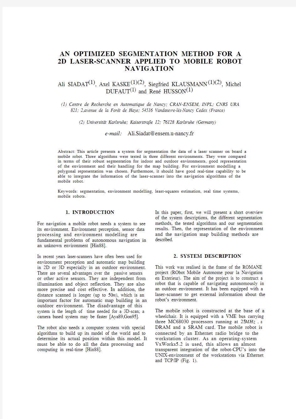
and TCP/IP (Fig. 1).
ROMANE
réseau des stations de travail
Fig. 1. Structure of ROMANE
The robot has several sensors. The odometer,gyrometer and magnetic compass are currently used to calculate the relative position of the robot while it is moving. This position determination process is done using the Kalman filter technique [Von96].
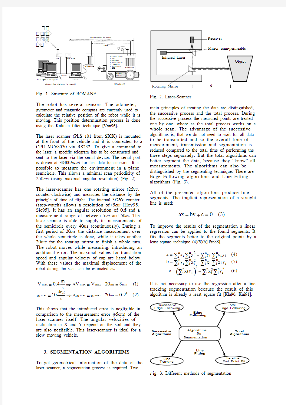
The laser scanner (PLS 101 from SICK) is mounted at the front of the vehicle and it is connected to a CPU MC68030 via RS232. To give a command to the laser, a specific telegram has to be constructed and sent to the laser via the serial device. The serial port is driven at 38400baud for fast data transmission. It is possible to measure the environment in a plane semicircle. This allows a minimal scan periodicity of 250ms (using maximal angular resolution) (Fig. 2).The laser-scanner has one rotating mirror (25Hz ,counter-clockwise) and measures the distance by the principle of time of flight. The internal 3GH z counter (stop-watch) allows a resolution of ±5cm [Hey95,Sic95]. It has an angular resolution of 0.5° and a measurement range of between 7cm and 50m . The laser-scanner is able to supply its measurements of the semicircle every 40ms (continuously). During a first period of 20ms the distance measurement over the whole semicircle is done, while it takes another 20ms for the rotating mirror to finish a whole turn.The robot moves while measuring, introducing an additional error. The maximal values for translation speed and angular velocity of cap are listed below.With these values the maximal displacement of the robot during the scan can be estimated as:
V max ?0.4
m
s ??V max ?V max ×20ms =8mm (1)ωmax ?10deg
s ??ωmax ?ωmax ×20ms =0.2o
(2)This shows that the introduced error is negligible in comparison to the measurement error (±5cm) of the laser-scanner itself. The angular velocities of inclination in X and Y depend on the soil and they are also negligible. This laser-scanner is ideal for a slow moving vehicle.
3. SEGMENTATION ALGORITHMS To get geometrical information of the data of the laser scanner, a segmentation process is required. Two
Fig. 2. Laser-Scanner
main principles of treating the data are distinguished,the successive process and the total process. During the successive process the measured points are treated one by one, where as the total process works on a whole scan. The advantage of the successive algorithms is, that we do not need to wait for all data to be transmitted and so the overall time of measurement, transmission and segmentation is reduced compared to the total time of performing the three steps separately. But the total algorithms can better segment the data, because they “know” all measurements. The algorithms can also be distinguished by the segmenting technique. There are Edge Following algorithms and Line Fitting algorithms (Fig. 3).
All of the presented algorithms produce line segments. The implicit representation of a straight line is used:
ax +by +c =0(3)
To improve the results of the segmentation a linear regression can be applied to the found segments. It fits the segments better to the original points by a least square technique (4)(5)(6)[Pre88].
a =i x i 2y ?i y i x i
y i n
∑i n ∑i n ∑i n ∑(4)b =i y i 2x ?i x i x i
y i n
∑i n ∑i n ∑i n ∑(5)c =
2
i x i y i n ∑(
)
?i 2x i n ∑i
2y i n ∑(6)
It is not necessary to use the regression after a line
tracking segmentation because the result of this algorithm is already a least square fit [Kla96, Kni91].
F ig. 3. Different methods of segmentation
4. TESTED ALGORITHMS
To chose the best algorithm for the data segmentation, three algorithms( Iterative End Point Fit "IEPF", Successive Edge Following "SEF" and Line Tracking "LT") were implemented and tested in different indoor and outdoor environments. The best algorithm should ensure a robust segmentation. This means that the number of segments should be as stable as possible against variations of the algorithm’s segmentation parameters, and as a second point the number of segments should be as stable as possible against variations from the complexity of the environment. Furthermore the algorithm must not create artefacts.
The SEF works directly on the distances measured by the laser-scanner (no transformation to x/y Cartesian co-ordinates). A segment is completed when the difference between a distance and his following distance exceeds a given threshold (Fig. 4).The LT does a linear regression over n-points . If the distance d n (the distance of the point P n to the already estimated straight line) is greater than a given threshold the end of a segment is found at the point (n-1) and a new segment starts (n is reset to 0). If not, we set n=n+1 and we restart with the linear regression (Fig. 5).
The IEPF is a recursive algorithm. A line defined by the first (P 0) and the last (P n ) point of the scan.Then the point with the maximum distance to this line is detected (P j ). This point divides the scan in two intervals and the algorithm starts recursively again until the maximum distance is smaller than a certain threshold (Fig. 6 & 7) [Cro89, Dud 73,
Kni91].
Fig. 4. SEF terminates a segment, if the difference
of two successive distances is greater than the threshold T ( |d4- d5| > T).
Fig. 5. LT terminates a segment if the distance of Pi
to the already estimated line is grater than the
threshold (d5>T).
P 0
P Fig. 6. IEPF algorithm searches the point P j with
the greatest distance to the straight line passing through P 0 and P n . If this distance dj is greater than the threshold T, the line P 0,P n
is broken into two lines P 0,P
j and P j , P
n and another segmentation step is applied for these two lines.
Fig. 7. IEPF segmentation of an indoor scan.
5. EXPERIMENTAL RESULTS SEF and LT algorithms are fast, but an important improvement is the adaptation of the threshold T to the absolute distance of the point. The minimal distance between two successive points has a linear dependency with the absolute distance of the point and also the measurement error depends on the
distance of the point to the laser scanner (Fig. 8).
Fig. 8. The distance of two successive points (?d1 &
?d2) depend on the distance of surface to the laser scanner (d1 & d2)
SEF normally doesn't need any pre-processing (Cartesian transformation). But linear regressing (post-processing) works on the Cartesian co-ordinate, so the pre-processing is necessary. For LT algorithm the post-processing is not necessary. It creates the least square fit segments.
IEPF is slower. It needs for pre- and post-processing and it must wait for all the data to be scanned (250 ms). But it is very robust in both indoor and outdoor environments.
The results of these algorithms for three different environments (complex indoor, less complex indoor and complex outdoor) are shown. All presented results are obtained on the mobile robot ROMANE which was following a pre-planed trajectory.
The measured computation times give a good idea of the real-time behaviour of the different algorithms. In the tables the row “T” shows the used threshold. The next four rows show the mean times of pre-processing, of segmentation, of post-processing and of the overall time total. The row “number of segments” shows the minimum, maximum and the mean number of segments in all scans. The mean value, s mean, is the most meaningful value. It shows in combination with the criterion visual. Therefore a good environment representation does not correlate to the number of segments. d mean is the geometric average of measure point-to-segment distances and d max is the average of the maximal error of every single scan. The user symbols express very good (++) to unacceptable (- -).
Table 1: Complex indoor environment (162 scans)
complex indoor environment
Algo-rithm T in
cm
computation time in ms no of segments error in cm visual
t pre t seg t post t total s min s mean s max d mean d max
SEF69.8 3.391.5105.369128.01980.360.70+
99.8 2.584.998.360116.71840.390.79+
1211.2 2.864.379.04691.11510.49 1.11++
1510.6 3.262.777.44487.31480.52 1.23+
2010.6 2.654.868.83473.31290.69 1.72+ IEPF48.9128.864.7203.75293.91350.58 1.07+ 610.7110.942.8164.92860.41010.90 1.81++
89.0103.637.4151.11748.887 1.13 2.40+
109.498.032.5141.71242.183 1.34 3.00+
1511.091.126.0129.1733.069 1.82 4.47o LT410.495.70.0107.03986.51440.96 1.92+ 610.173.70.084.72150.796 2.16 4.90+
811.066.70.078.31338.275 3.428.52o
109.563.50.074.0831.663 4.8012.78o
1511.058.40.069.8623.3438.0824.06o Table 2: Structured indoor environment (110 scans)
less complex indoor environment
Algo-rithm T in
cm
computation time in ms no of segments error in cm visual
t pre t seg t post t total s min s mean s max d mean d max
SEF610.2 3.170.484.96196.61320.270.53+ 910.5 4.065.580.26090.01190.270.54+
128.5 3.147.159.83461.4840.280.72++
1512.4 2.743.859.53469.2820.290.75o
2011.5 2.936.552.02647.4620.42 1.13-IEPF411.1121.543.8177.31758.8760.66 1.30+ 611.180.720.5113.5823.244 1.11 2.48++
810.461.115.188.0412.625 1.40 3.50+
108.952.912.575.338.718 1.63 4.33+
1510.046.010.467.33 6.613 1.99 5.55o LT410.071.10.082.21542.7680.70 1.66+ 610.255.10.066.2616.734 1.14 3.04+
810.051.60.062.539.518 1.74 4.85+
108.950.50.061.137.314 2.35 6.67o
159.350.40.060.73 5.411 3.6814.47o Table 3: Complex outdoor environment (110 scans)
complex outdoor environment
Algo-
rithm
T in
cm
computation time in ms no. of segments error in cm visual
t pre t seg t post t total s min s mean s max d mean d max
SEF159.9 1.7100.6113.484147.01890.500.93++ 209.4 1.384.696.560
117.91580.75 1.56+ 258.6 2.073.485.15098.5134 1.06 2.37o
308.6 2.660.773.44790.0126 1.41 3.22-
358.3 2.454.166.24275.2118 1.78 4.04--IEPF108.465.157.2132.84965.591 1.17 2.20++ 158.860.950.3120.74456.276 1.64 3.19++
208.861.734.9107.93849.063 2.15 4.28++
308.856.131.798.03039.253 3.407.20+
408.146.228.483.72332.346 4.4710.48o LT109.075.00.085.74963.289 1.67 3.52++ 1511.266.20.079.43650.366 3.507.82+
209.563.90.074.73142.858 5.8014.20o
309.560.80.071.62836.14711.6833.50-
409.753.60.065.01726.23417.0847.06-
6. ENVIRONMENT REPRESENTATION
A model or representation of the world can be created
To avoid the further usage of explicit representations the vector form is used. Instead of the points P 1 and P 2 the vectors V 1 and V 2 are defined. To speed up position correction and map construction algorithms,some other informations about the line segment are held. These are the direction vector, the normal vector, the length of the segment, the number of points, and its perpendicular distance to the origin. In this representation a segment requires 48 bytes of memory (Fig. 10).
The implicit representation allows also a very fast calculation of the point-to-line distance. Firstly we need the normalised version of eq. (2):
ax i +by i +c ()
2a +2
b (7)
and the normalised parameters:
?a =a 2a +2
b ?b =b 2a +2b ?c
=c 2a +2
b (8)
We obtained an oriented distance from the following equation:
d i =?a
x i +?by i +?c (9)Oriented distance implies that the distance is a signed
value depending on whether the point P i
is located between the origin of the co-ordinate system and the line (d i <0), or on the outer side (d
i >0) . This may be important information in a further step of
automatic map building.
Fig .10. Vector representation.
7. NAVIGATION MAP
For the construction of a map, it is very important to have a correct position and orientation of the robot at all times. We already use an internal localisation algorithm for tracking of position and orientation [Von96]. This method accumulates the errors in movement and is very sensitive to slipping.Therefore the error between the real position and estimated position increases when the robot moves.To correct these errors, external information must be used. In our case, laser data are employed for guiding and for building a navigation map (Fig. 11).The basic navigation map is the first segmented scan. Successively, we can terminate the position and orientation errors by correlating the present laser image and last navigation map. The new segments of laser image can be merged in the last navigation map.
We are interested in the segment based correlation techniques. Our current work is testing two correlation methods. The first is a correlation between the segmented navigation map and a segmented laser image and the second consists of the correlation between the segmented navigation map and a no-segmented laser data.
For the segment-segment correlation method IEPF algorithm is not fast enough. SEF and LT create many segments and they are not optimised for this method. Now, we are testing the segment- point correlation techniques. In this case, the laser data segmentation task can be executed both the correlation task and at the end, the segmented laser image can be used for update to our navigation map.A Point-Point correlation method is also tested. It is not very fast and also it is not compatible for segmented navigation map building [Wei94].
localisation algorithm.
8. CONCLUSIONS
For the ROMANE perception of environment, we have chosen an industrial 2D laser-scanner. It is fast, robust, low in cost and precise enough for our application. The multi-task operating system (vxWorks) and three independent CPU allow the execution of several algorithms for processing the laser data; such as environment perception, data segmentation, environment modelling and laser based navigation in real time.
The segment based algorithms for the above tasks are usually faster and the segmented maps take up less memory. Therefore we have developed and tested several segmentation algorithms.
"Iterative End Point Fit" algorithm gives the best result and it is ideal for environment representation and building navigation maps. But it is too slow (overall time = 150ms calculation time + 250ms scan time = 400ms) for laser based navigation and position estimation. "Line Tracking" and "Successive Edge Following" give bad segmentation in certain environments. The threshold criteria must be changed for each environment, on the other hand they are fast enough for real time navigation.
Our current work is building the real time 2D navigation map, the fusion of the laser data with vision data for 3D perception and developing a 3D laser system relying on the same principles and hypothesis.
This system will be used in a co-operation project with APF ( Association des Paralysés de France) for developing a semi-autonomous wheelchair for physically disable people.
9. REFERENCES
[Ayache N., Faugeras O. D. (1989)]. Maintaining Representations of the Environment of a Mobile Robot. IEEE Transactions on Robotics and Automation, vol. 5, no. 6, p. 804-819. [Crowley J.L.. (1989)]. World Modeling and Position Estimation for a Mobile Robot Using Ultrasonic Ranging. Int. Conf. Robotics and Automation, p.674-680.
[Duda R.O. and Hart P.E.. (1973)]. Pattern Classification and Scene Analysis. John Wiley & Sons, Inc.
[Gonzalez J., Ollero A., Reina A. (1994)]. Map Building for a Mobile Robot equipped with a 2D Laser Rangefinder, IEEE, p. 1904-1909,1994. [Gonzalez J., Stentz A., Reina A. (1995)]. A Mobile Robot Iconic Estimator Using a Radial Laser Scanner. Journal of Intelligent and Robotic Systems 13, p.161-179, 1995. Kluwer Academic Publishers, Netherlands.
[Heyrowsky F., Kerprich D. (1995)]. Erweiterung eines Laserscanners auf r?umliche Abtastung und Integration in die Navigationssensorik eines
“Autonomen Mobilen Systems”. Diplomarbeit, Fachhochschule Bochum 1995, Fachbereich Elektrotechnik / Nachrichtentechnik.
[Hinkel R., Knieriemen T. (1988)]. Environment Perception With A Laser Radar in a Fast Moving Robot. IFAC Robot Control, Kalsruhe FRG, P.
271-277.
[Klausmann S. (1996)]. Segmentierung und auswertung der daten eines laserscanners für die navigation eines mobilen autonomen roboters.
Diplomarbeit, Institut für prozebrechentechnik und robotik, Universit?t Karlsruhe. [Knieriemen T. (1991)]. Autonome Mobile Roboter: Sensordateninterpretation und Weltmodellierung zur Navigation in unbekannter Umgebung. Bd.
80 aus der Reihe Informatik; BI-
Wissenschaftsverlag.
[Press W. H., Flannery B. P., Teukolsky S. A. and Vertterling W. T. (1988)]. Numerical Recipes in
C. Cambridge University Press.
[Sick (1995)]. Sick PLS Laser Scanner Operating Instructions. Erwin Sick GmbH; Optik-Elektronik; Waldkirch, Germany.
[Von der Hardt H. , Wolf D. , Husson R. (1996)].
The dead reckoning localization system of the wheeled mobile robot ROMANE.
IEEE/SICE/RSJ, P. 603-610.
[Weib G., Wetzler C., Puttkamer E. (1994)] Keeping Track of Position and Orientation of moving Indoor Systems by Correlation of Range-Finder Scans. University of Kaiserslautern, Germany.