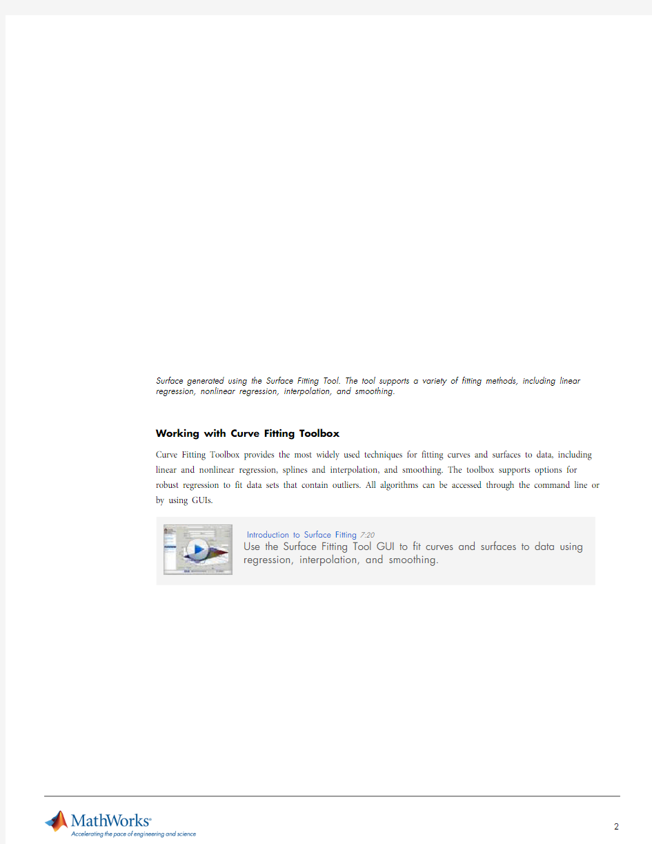
Surface generated using the Surface Fitting Tool. The tool supports a variety of fitting methods, including linear regression, nonlinear regression, interpolation, and smoothing.
Working with Curve Fitting Toolbox
Curve Fitting Toolbox provides the most widely used techniques for fitting curves and surfaces to data, including linear and nonlinear regression, splines and interpolation, and smoothing. The toolbox supports options for robust regression to fit data sets that contain outliers. All algorithms can be accessed through the command line or by using GUIs.
Introduction to Surface Fitting7:20
Use the Surface Fitting Tool GUI to fit curves and surfaces to data using
regression, interpolation, and smoothing.
Fitting multiple candidate models to a single data series using the Surface Fitting Tool. You can compare the fitted surfaces visually or use goodness-of-fit metrics such as R2, adjusted R2, sum of the squared errors, and root mean squared error.
Fitting Data with GUIs
The Curve Fitting Tool GUI and Surface Fitting Tool GUI simplify common tasks that include:
?Importing data from the MATLAB?workspace
?Visualizing your data to perform exploratory data analysis
?Generating fits using multiple fitting algorithms
?Evaluating the accuracy of your models
?Performing postprocessing analysis that includes interpolation and extrapolation, generating confidence intervals, and calculating integrals and derivatives
?Exporting fits to the MATLAB workspace for further analysis
?Automatically generating MATLAB code to capture work and automate tasks
MATLAB function generated with the Surface Fitting Tool.
Working at the Command Line
Working at the command line lets you develop custom functions for analysis and visualization. These functions enable you to:
?Duplicate your analysis with a new data set
?Replicate your analysis with multiple data sets (batch processing)
?Embed a fitting routine into MATLAB functions
?Extend the base capabilities of the toolbox
Curve Fitting Toolbox provides a simple intuitive syntax for command-line fitting, as in the following examples:
?Linear Regression:fittedmodel = fit([X,Y], Z, ’poly11’);
?Nonlinear Regression:fittedmodel = fit(X, Y, ’fourier2’);
?Interpolation:fittedmodel = fit([Time,Temperature], Energy, ’cubicinterp’);?Smoothing:fittedmodel = fit([Time,Temperature], Energy, ’lowess’, ‘span’,
0.12);
The results of a fitting operation are stored in an object called“fittedmodel.”Postprocessing analysis, such as plotting, evaluation, and calculating integrals and derivatives, can be performed by applying a method to this object, as in these examples:
?Plotting:plot(fittedmodel)
?Differentiation:differentiate(fittedmodel, X, Y)
?Evaluation:fittedmodel(80, 40)
Curve Fitting Toolbox lets you move from GUIs to the command line. Using the GUIs, you can generate MATLAB functions that duplicate any GUI-based analysis. You can also create fit objects within the GUI and export them to the MATLAB workspace for further analysis.
Extending the capabilities of the toolbox with a custom visualization. The color of the heat map corresponds to the deviation between the fitted surface and a reference model.
Regression
Curve Fitting Toolbox supports linear and nonlinear regression.
Linear Regression
The toolbox supports over 100 regression models, including:
?Lines and planes
?High order polynomials (up to ninth degree for curves and fifth degree for surfaces)
?Fourier and power series
?Gaussians
?Weibull functions
?Exponentials
?Rational functions
?Sum of sines
All of these standard regression models include optimized solver parameters and starting conditions to improve fit quality. Alternatively, you can use the Custom Equation option to specify your own regression model.
In the GUIs you can generate fits based on complicated parametric models by using a drop-down menu. At the
command line you can access the same models using intuitive names.
(top, left) or select a second-order Fourier series in the Fit Editor (top, right).
input a MATLAB function.
The regression analysis options in Curve Fitting Toolbox enable you to:
?Choose between two types of robust regression: bisquare or least absolute residual
?Specify starting conditions for the solvers
?Constrain regression coefficients
?Choose Trust-Region or Levenberg-Marquardt algorithms
Fit Options GUI in the Surface Fitting Tool. You can control the type of robust regression, the choice of optimization solver, and the behavior of the optimization solver with respect to starting conditions and constraints.
Splines and Interpolation
Curve Fitting Toolbox supports a variety of interpolation methods, including B-splines, thin plate splines, and tensor product splines. Curve Fitting Toolbox provides functions for advanced spline operations, including break/ knot manipulation, optimal knot placement, and data-point weighting.
A cubic B-spline and the four polynomials from which it is made. Splines are smooth piecewise polynomials used to represent functions over large intervals.
You can represent a polynomial spline in ppform and B-form. The ppform describes the spline in terms of breakpoints and local polynomial coefficients, and is useful when the spline will be evaluated extensively. The B-form describes a spline as a linear combination of B-splines, specifically the knot sequence and B-spline coefficients.
Curve Fitting Toolbox also supports other types of interpolation, including:
?Linear interpolation
?Nearest neighbor interpolation
?Piecewise cubic interpolation
?Biharmonic surface interpolation
?Piecewise Cubic Hermite Interpolating Polynomial (PCHIP)
The Curve Fitting Toolbox commands for constructing spline approximations accommodate vector-valued
gridded data, enabling you to create curve and surfaces in any number of dimensions.
Linear interpolation using the Surface Fitting Tool.
Smoothing
Smoothing algorithms are widely used to remove noise from a data set while preserving important patterns. Curve Fitting Toolbox supports both smoothing splines and localized regression, which enable you to generate a
predictive model without specifying a functional relationship between the variables.
Localized regression model. Smoothing techniques can be used to generate predictive models without specifying a parametric relationship between the variables.
Nonparametric Fitting4:08
Develop a predictive model when you can’t specify a function that
describes the relationship between variables.
Curve Fitting Toolbox supports localized regression using either a first-order polynomial (lowess) or a second-order polynomial (loess). The toolbox also provides options for robust localized regression to accommodate outliers in the data set. Curve Fitting Toolbox also supports moving average smoothers such as Savitzky-Golay filters.
Exploratory data analysis using a Savitzky-Golay filter. Smoothing data enables you to identify periodic components.
Previewing and Preprocessing Data
Curve Fitting Toolbox supports a comprehensive workflow that progresses from exploratory data analysis (EDA) through model development and comparison to postprocessing analysis.
You can plot a data set in two or three dimensions. The toolbox provides options to remove outliers, section data series, and weight or exclude data points.
Curve Fitting Toolbox lets you automatically center and scale a data set to normalize the data and improve fit quality. The Center and scale option can be used when there are dramatic differences in variable scales or the
distance between data points varies across dimensions.
Normalizing data with the Center and scale option to improve fit quality.
Outlier exclusion using the Curve Fitting Tool (top). You can create exclusion rules (middle) to remove all data points that match some specific criteria, and use the graphical exclusion option (bottom) to click on a data point and remove
it from the sample.
Weighting data points using the Surface Fitting Tool.
Developing, Comparing, and Managing Models
Curve Fitting Toolbox lets you fit multiple candidate models to a data set. You can then evaluate goodness of fit using a combination of descriptive statistics, visual inspection, and validation.
Descriptive Statistics
Curve Fitting Toolbox provides a wide range of descriptive statistics, including:
?R-square and adjusted R-square
?Sum of squares due to errors and root mean squared error
?Degrees of freedom
The Table of Fits lists all of the candidate models in a sortable table, enabling you to quickly compare and contrast
multiple models.
The Surface Fitting Tool, which provides a sortable table of candidate models.
Visual Inspection of Data
The toolbox enables you to visually inspect candidate models to reveal problems with fit that are not apparent in summary statistics. For example, you can:
?Generate side-by-side surface and residual plots to search for patterns in the residuals
?Simultaneously plot multiple models to compare how well they fit the data in critical regions
?Plot the differences between two models as a new surface
Surface generated with the Surface Fitting Tool. The color of the heat map corresponds to the deviation between the fitted surface and a reference model.
Validation Techniques
Curve Fitting Toolbox supports validation techniques that help protect against overfitting. You can generate a predictive model using a training data set, apply your model to a validation data set, and then evaluate goodness of fit.
Postprocessing Analysis
Once you have selected the curve or surface that best describes your data series you can perform postprocessing analysis. Curve Fitting Toolbox enables you to:
?Create plots
?Use your model to estimate values (evaluation)
?Calculate confidence intervals
?Create prediction bounds
?Determine the area under your curve (integration)
?Calculate derivatives
Postprocessing analysis with the Curve Fitting Tool, which automatically creates a scatter plot of the raw data along with the fitted curve. The first and second derivatives of the fitted curve are also displayed.
The following examples show how postprocessing at the command line applies intuitive commands to the objects created from a fitting operation:
?Evaluation:EnergyConsumption = fittedmodel(X, Y)
?Plotting:EnergySurface = plot(fittedmodel)
?Integration:Volume_Under_Surface = quad2d(fittedmodel, Min_X, Max_X, Min_Y, Max_Y)
?Differentiation:Gradient = differentiate(fittedmodel, X,Y)
?Computing confidence intervals: Confidence_Intervals = confint(fittedmodel)
Product Details, Demos, and System Requirements
https://www.doczj.com/doc/f412654688.html,/products/curvefitting
Trial Software
https://www.doczj.com/doc/f412654688.html,/trialrequest
Sales
https://www.doczj.com/doc/f412654688.html,/contactsales
Technical Support
https://www.doczj.com/doc/f412654688.html,/support Using command-line postprocessing to calculate and plot a gradient.
Resources
Online User Community https://www.doczj.com/doc/f412654688.html,/matlabcentral Training Services https://www.doczj.com/doc/f412654688.html,/training Third-Party Products and Services https://www.doczj.com/doc/f412654688.html,/connections Worldwide Contacts https://www.doczj.com/doc/f412654688.html,/contact
至于工具箱的安装说明参见: https://www.doczj.com/doc/f412654688.html,/viewthread.php?tid=120&page=1&fromuid=4481#p id123 Maplesoft《Maple Toolbox for MATLAB》 https://www.doczj.com/doc/f412654688.html,/thread-236-1-1.html Sergiy Iglin《Graph Theory Toolbox》(图论工具 箱)https://www.doczj.com/doc/f412654688.html,/thread-295-1-1.html Koert Kuipers《Branch And Bound toolbox 2.0》(BNB20分支定界工具 箱)https://www.doczj.com/doc/f412654688.html,/thread-226-1-1.html Howard Wilson《Numerical Integration Toolbox》(NIT数值积分工具 箱)https://www.doczj.com/doc/f412654688.html,/thread-225-1-1.html Anton Zaicenco《FEM toolbox for solid mechanics》(固体力学有限元工具箱)https://www.doczj.com/doc/f412654688.html,/thread-219-1-1.html Nicholas J. Higham《The Matrix Computation Toolbox》(矩阵计算工具箱) https://www.doczj.com/doc/f412654688.html,/thread-422-1-1.html Paolo Di Prodi《robotic toolbox》(机器人工具 箱)https://www.doczj.com/doc/f412654688.html,/thread-274-1-1.html Moein Mehrtash《GPS Navigation Toolbox 》(GPS导航工具箱) https://www.doczj.com/doc/f412654688.html,/thread-228-1-1.html J.Divahar 《Airfoil_Analyzer_toolbox》(翼型分析工具箱) https://www.doczj.com/doc/f412654688.html,/thread-218-1-1.html Rasmus Anthin《Multivariable Calculus Toolbox 》(多变量微积分工具 箱)https://www.doczj.com/doc/f412654688.html,/thread-251-1-1.html 《Time frequency analysis toolbox》(时频分析工具 箱)https://www.doczj.com/doc/f412654688.html,/thread-439-1-1.html
m a t l a b优化工具箱介 绍
matlab优化工具箱介绍 分类: Matlab2007-11-03 20:27 6405人阅读评论(0) 收藏举报在生活和工作中,人们对于同一个问题往往会提出多个解决方案,并通过各方面的论证从中提取最佳方案。最优化方法就是专门研究如何从多个方案中科学合理地提取出最佳方案的科学。由于优化问题无所不在,目前最优化方法的应用和研究已经深入到了生产和科研的各个领域,如土木工程、机械工程、化学工程、运输调度、生产控制、经济规划、经济管理等,并取得了显著的经济效益和社会效益。 用最优化方法解决最优化问题的技术称为最优化技术,它包含两个方面的内容: 1)建立数学模型即用数学语言来描述最优化问题。模型中的数学关系式反映了最优化问题所要达到的目标和各种约束条件。 2)数学求解数学模型建好以后,选择合理的最优化方法进行求解。 最优化方法的发展很快,现在已经包含有多个分支,如线性规划、整数规划、非线性规划、动态规划、多目标规划等。 9.1 概述 利用Matlab的优化工具箱,可以求解线性规划、非线性规划和多目标规划问题。具体而言,包括线性、非线性最小化,最大最小化,二次规划,半无限问题,线性、非线性方程(组)的求解,线性、非线性的最小二乘问题。另外,该工具箱还提供了线性、非线性最小化,方程求解,曲线拟合,二次规划等问
5.大型方法的演示函数
9.1.3 参数设置 利用optimset函数,可以创建和编辑参数结构;利用optimget函数,可以获得options优化参数。 ● optimget函数 功能:获得options优化参数。 语法: val = optimget(options,'param') val = optimget(options,'param',default) 描述: val = optimget(options,'param') 返回优化参数options中指定的参数的 值。只需要用参数开头的字母来定义参数就行了。 val = optimget(options,'param',default) 若options结构参数中没有定义 指定参数,则返回缺省值。注意,这种形式的函数主要用于其它优化 函数。 举例:
matlab工具箱如何安装 在matlab的file下面的set path把它加上,把路径加进去后在: file→Preferences→General的Toolbox Path Caching里点击update Toolbox Path Cache更新一下。 以下是我在别的地方看到的,转过来你参考一下吧。 首先说说添加到matlab搜索路径好处:1 对n——你只需要存储一个副本,就可以在其他地方使用。具体来说,假设你在数据盘D上新建了两个目录abc和def,这两个工程(每个目录下的所有程序相应地称为一个工程)都需要调用同一个(些)函数(简称工具箱),这时候,如果你没有把该工具箱添加到matlab 的搜索路径下,则需要分别把工具箱中所有用到的文件都复制到目录abc和def下才能正确运行。这显然浪费空间,所以,matlab提供了一个搜索路径(默认在matlab安装目录下的toolbox中),只要把工具箱对应的整个文件夹复制到搜索路径对应的目录下,并且通知matlab一声(把该路径正确添加到搜索路径中),就可以在abc和def中使用这个工具箱了(即无论你的工程文件在哪个目录(有效的目录)下都可以访问这个工具箱中的函数)。下面就以matlab安装目录下的toolbox目录作为默认的添加路径进行详细说明。 1. 如何添加工具箱? 以下是添加工具箱的方法: 如果是Matlab安装光盘上的工具箱,重新执行安装程序,选中即可。如果是单独下载的工具箱,则需要把新的工具箱(以下假设工具箱名字为svm)解压到toolbox目录下,然后用addpath或者pathtool 把该工具箱的路径添加到matlab的搜索路径中,最后用which newtoolbox_command.m来检验是否可以访问。如果能够显示新设置的路径,则表明该工具箱可以使用了。具体请看工具箱自己代的README 文件。 1.1 举例: 要添加的工具箱为svm,则解压后,里边有一个目录svm,假设matlab安装在D:\MATLAB6p5,将svm目录拷贝至D:\MATLAB6p5\toolbox,然后运行matlab,在命令窗口输入addpath D:\MATLAB6p5\toolbox\svm回车,来添加路径。然后在svm目录下,任意找一个m文件,以svcinfo.m 为例,在命令窗口中输入which svcinfo.m。如果显示出该文件路径,如D:\MATLAB6p5\toolbox\svm\svcinfo.m,则安装成功,当然也可以在命令窗口输入path来查看。 上面的说明和例子基本上介绍了在matlab中如何添加工具箱,下面是其他补充: 1.2 添加方式总结: 事实上,有两种添加工具箱到matlab搜索路径的方法:其一是用代码,其二是用界面。其实无论用哪种方法,都是修改pathdef.m这个文件,阁下如果是高手,可以直接打开该文件修改,呵呵,对此这里不作讨论。 1.2.1 代码方式: 适用于添加下载的工具箱(别人的): 在命令窗口输入addpath D:\MATLAB6p5\toolbox\svm 或者addpath(‘D:\MATLAB6p5\toolbox\svm’); 但是这种方法只能添加svm目录,如果该目录下有其他子文件夹,并且运行时候“隐式”调用到这些子文件夹(例如假设svm目录下存在子文件夹matdata,该子文件夹下有logo.mat这个文件,且在m文件代码中使用了诸如load logo 这样的句子,即没有显式给出logo.mat的具体路径,则称为“隐式”),则不能正确访问。因此,有必要在添加时使用以下语句把svm目录下所有文件夹都添加到搜索路径中:500){this.resized=true;;}"> 程序代码 addpath(genpath(D:\MATLAB6p5\toolbox\svm)); 另外,如果只使用以上代码,则退出matlab后,新添加的路径不会被保存下来,下次重新启动matlab
云南大学数学与统计学实验教学中心 实验报告 一、实验目的 1.熟悉MATLAB的运行环境. 2.学会初步建立数学模型的方法 3.运用回归分析方法来解决问题 二、实验内容 实验一:某公司出口换回成本分析 对经营同一类产品出口业务的公司进行抽样调查,被调查的13家公司,其出口换汇成本与商品流转费用率资料如下表。试分析两个变量之间的关系,并估计某家公司商品流转费用率是6.5%的出口换汇成本. 实验二:某建筑材料公司的销售量因素分析 下表数据是某建筑材料公司去年20个地区的销售量(Y,千方),推销开支、实际帐目数、同类商品
竞争数和地区销售潜力分别是影响建筑材料销售量的因素。1)试建立回归模型,且分析哪些是主要的影响因素。2)建立最优回归模型。 提示:建立一个多元线性回归模型。
三、实验环境 Windows 操作系统; MATLAB 7.0. 四、实验过程 实验一:运用回归分析在MATLAB 里实现 输入:x=[4.20 5.30 7.10 3.70 6.20 3.50 4.80 5.50 4.10 5.00 4.00 3.40 6.90]'; X=[ones(13,1) x]; Y=[1.40 1.20 1.00 1.90 1.30 2.40 1.40 1.60 2.00 1.00 1.60 1.80 1.40]'; plot(x,Y,'*'); [b,bint,r,rint,stats]=regress(Y,X,0.05); 输出: b = 2.6597 -0.2288 bint = 1.8873 3.4322 -0.3820 -0.0757 stats = 0.4958 10.8168 0.0072 0.0903 即==1,0?6597.2?ββ,-0.2288,0?β的置信区间为[1.8873 3.4322],1,?β的置信区间为[-0.3820 -0.0757]; 2r =0.4958, F=10.8168, p=0.0072 因P<0.05, 可知回归模型 y=2.6597-0.2288x 成立. 1 1.5 2 2.5 散点图 估计某家公司商品流转费用率是6.5%的出口换汇成本。将x=6.5代入回归模型中,得到 >> x=6.5; >> y=2.6597-0.2288*x y = 1.1725
matlab建立多元线性回归模型并进行显着性检验及预测问题 例子; x=[143 145 146 147 149 150 153 154 155 156 157 158 159 160 162 164]'; X=[ones(16,1) x]; 增加一个常数项Y=[88 85 88 91 92 93 93 95 96 98 97 96 98 99 100 102]'; [b,bint,r,rint,stats]=regress(Y,X) 得结果:b = bint = stats = 即对应于b的置信区间分别为[,]、[,]; r2=, F=, p= p<, 可知回归模型y=+ 成立. 这个是一元的,如果是多元就增加X的行数! function [beta_hat,Y_hat,stats]=regress(X,Y,alpha) % 多元线性回归(Y=Xβ+ε)MATLAB代码 %? % 参数说明 % X:自变量矩阵,列为自变量,行为观测值 % Y:应变量矩阵,同X % alpha:置信度,[0 1]之间的任意数据 % beta_hat:回归系数 % Y_beata:回归目标值,使用Y-Y_hat来观测回归效果 % stats:结构体,具有如下字段 % =[fV,fH],F检验相关参数,检验线性回归方程是否显着 % fV:F分布值,越大越好,线性回归方程越显着 % fH:0或1,0不显着;1显着(好) % =[tH,tV,tW],T检验相关参数和区间估计,检验回归系数β是否与Y有显着线性关系 % tV:T分布值,beta_hat(i)绝对值越大,表示Xi对Y显着的线性作用% tH:0或1,0不显着;1显着 % tW:区间估计拒绝域,如果beta(i)在对应拒绝区间内,那么否认Xi对Y显着的线性作用 % =[T,U,Q,R],回归中使用的重要参数 % T:总离差平方和,且满足T=Q+U % U:回归离差平方和 % Q:残差平方和 % R∈[0 1]:复相关系数,表征回归离差占总离差的百分比,越大越好% 举例说明 % 比如要拟合y=a+b*log(x1)+c*exp(x2)+d*x1*x2,注意一定要将原来方程线化% x1=rand(10,1)*10; % x2=rand(10,1)*10; % Y=5+8*log(x1)+*exp(x2)+*x1.*x2+rand(10,1); % 以上随即生成一组测试数据 % X=[ones(10,1) log(x1) exp(x2) x1.*x2]; % 将原来的方表达式化成Y=Xβ,注意最前面的1不要丢了
robotic toolbox for matlab工具箱下载地址: https://www.doczj.com/doc/f412654688.html,/source/940770 1. PUMA560的MATLAB仿真 要建立PUMA560的机器人对象,首先我们要了解PUMA560的D-H参数,之后我们可以利用Robotics Toolbox工具箱中的link和robot函数来建立 PUMA560的机器人对象。 其中link函数的调用格式: L = LINK([alpha A theta D]) L =LINK([alpha A theta D sigma]) L =LINK([alpha A theta D sigma offset]) L =LINK([alpha A theta D], CONVENTION) L =LINK([alpha A theta D sigma], CONVENTION) L =LINK([alpha A theta D sigma offset], CONVENTION) 参数CONVENTION可以取‘standard’和‘modified’,其中‘standard’代表采用标准的D-H参数,‘modified’代表采用改进的D-H参数。参数‘alpha’代表扭转角,参数‘A’代表杆件长度,参数‘theta’代表关节角,参数‘D’代表横距,参数‘sigma’代表关节类型:0代表旋转关节,非0代表移动关节。另外LINK还有一些数据域: LINK.alpha %返回扭转角 LINK.A %返回杆件长度 LINK.theta %返回关节角 LINK.D %返回横距 LINK.sigma %返回关节类型 LINK.RP %返回‘R’(旋转)或‘P’(移动) LINK.mdh %若为标准D-H参数返回0,否则返回1 LINK.offset %返回关节变量偏移 LINK.qlim %返回关节变量的上下限[min max] LINK.islimit(q) %如果关节变量超限,返回-1, 0, +1 LINK.I %返回一个3×3 对称惯性矩阵
回归分析MATLAB 工具箱 一、多元线性回归 多元线性回归:p p x x y βββ+++=...110 1、确定回归系数的点估计值: 命令为:b=regress(Y , X ) ①b 表示???? ?? ????????=p b βββ?...??10 ②Y 表示????????????=n Y Y Y Y (2) 1 ③X 表示??? ??? ????? ???=np n n p p x x x x x x x x x X ...1......... .........1 (12) 1 22221 11211 2、求回归系数的点估计和区间估计、并检验回归模型: 命令为:[b, bint,r,rint,stats]=regress(Y ,X,alpha) ①bint 表示回归系数的区间估计. ②r 表示残差. ③rint 表示置信区间. ④stats 表示用于检验回归模型的统计量,有三个数值:相关系数r 2、F 值、与F 对应的概率p. 说明:相关系数2 r 越接近1,说明回归方程越显著;)1,(1-->-k n k F F α时拒绝0H ,F 越大,说明回归方程越显著;与F 对应的概率p α<时拒绝H 0,回归模型成立. ⑤alpha 表示显著性水平(缺省时为0.05) 3、画出残差及其置信区间. 命令为:rcoplot(r,rint) 例1.如下程序. 解:(1)输入数据. x=[143 145 146 147 149 150 153 154 155 156 157 158 159 160 162 164]'; X=[ones(16,1) x]; Y=[88 85 88 91 92 93 93 95 96 98 97 96 98 99 100 102]'; (2)回归分析及检验. [b,bint,r,rint,stats]=regress(Y ,X) b,bint,stats 得结果:b = bint =
1、 考察温度x 对产量y 的影响,测得下列10组数据: 区间(置信度95%). x=[20:5:65]'; Y=[13.2 15.1 16.4 17.1 17.9 18.7 19.6 21.2 22.5 24.3]'; X=[ones(10,1) x]; plot(x,Y,'r*'); [b,bint,r,rint,stats]=regress(Y,X); b,bint,stats; rcoplot(r,rint) %残差分析,作残差图 结果: b = 9.1212 0.2230 bint = 8.0211 10.2214 0.1985 0.2476 stats = 0.9821 439.8311 0.0000 0.2333 即01 ??9.1212,0.2230ββ==;0?β的置信区间为[8.0211,10.2214]1?β的置信区间为[0.1985,0.2476]; 2r =0.9821 , F=439.831, p=0.0000 ,p<0.05, 可知回归模型 y=9.1212+0.2230x 成立. 将x=42带入得到18.4872.
从残差图可以看出,所有数据的残差离零点均较近,且残差的置信区间均包含零点,这说明回归模型y=9.1212+0.2230x能较好的符合原始数据。 2 某零件上有一段曲线,为了在程序控制机床上加工这一零件,需要求这段曲线的解析表达式,在曲线横坐标xi处测得纵坐标yi共11对数据如下: 求这段曲线的纵坐标y关于横坐标x的二次多项式回归方程。 t=0:2:20; s=[0.6 2.0 4.4 7.5 11.8 17.1 23.3 31.2 39.6 49.7 61.7]; T=[ones(11,1) ,t',(t.^2)']; [b,bint,r,rint,stats]=regress(s',T); b,stats; Y=polyconf(p,t,S) plot(t,s,'k+',t,Y,'r') %预测及作图 b = 1.0105 0.1971 0.1403
MATLAB---回归预测模型 Matlab统计工具箱用命令regress实现多元线性回归,用的方法是最小二乘法,用法是: b=regress(Y,X) [b,bint,r,rint,stats]=regress(Y,X,alpha) Y,X为提供的X和Y数组,alpha为显著性水平(缺省时设定为0.05),b,bint 为回归系数估计值和它们的置信区间,r,rint为残差(向量)及其置信区间,stats是用于检验回归模型的统计量,有四个数值,第一个是R2,第二个是F,第三个是与F对应的概率 p ,p <α拒绝 H0,回归模型成立,第四个是残差的方差 s2 。 残差及其置信区间可以用 rcoplot(r,rint)画图。 例1合金的强度y与其中的碳含量x有比较密切的关系,今从生产中收集了一批数据如下表 1。 先画出散点图如下: x=0.1:0.01:0.18; y=[42,41.5,45.0,45.5,45.0,47.5,49.0,55.0,50.0]; plot(x,y,'+') 可知 y 与 x 大致上为线性关系。
设回归模型为 y =β 0 +β 1 x 用regress 和rcoplot 编程如下: clc,clear x1=[0.1:0.01:0.18]'; y=[42,41.5,45.0,45.5,45.0,47.5,49.0,55.0,50.0]'; x=[ones(9,1),x1]; [b,bint,r,rint,stats]=regress(y,x); b,bint,stats,rcoplot(r,rint) 得到 b =27.4722 137.5000 bint =18.6851 36.2594 75.7755 199.2245 stats =0.7985 27.7469 0.0012 4.0883 即β 0=27.4722 β 1 =137.5000 β0的置信区间是[18.6851,36.2594], β1的置信区间是[75.7755,199.2245]; R2= 0.7985 , F = 27.7469 , p = 0.0012 , s2 =4.0883 。 可知模型(41)成立。 观察命令 rcoplot(r,rint)所画的残差分布,除第 8 个数据外其余残差的置信区间均包含零点第8个点应视为异常点,
本次教程的主要内容包含: 一、多元线性回归 2# 多元线性回归:regress 二、多项式回归 3# 一元多项式:polyfit或者polytool 多元二项式:rstool或者rsmdemo 三、非线性回归 4# 非线性回归:nlinfit 四、逐步回归 5# 逐步回归:stepwise 一、多元线性回归 多元线性回归: 1、b=regress(Y, X ) 确定回归系数的点估计值
2、[b, bint,r,rint,stats]=regress(Y,X,alpha)求回归系数的点估计和区间估计、并检验回归模型 ①bint表示回归系数的区间估计. ②r表示残差 ③rint表示置信区间 ④stats表示用于检验回归模型的统计量,有三个数值:相关系数r2、F值、与F对应的概率p 说明:相关系数r2越接近1,说明回归方程越显著;时拒绝H0,F越大,说明回归方程越显著;与F对应的概率p<α时拒绝H0 ⑤alpha表示显著性水平(缺省时为0.05) 3、rcoplot(r,rint)画出残差及其置信区间 具体参见下面的实例演示 4、实例演示,函数使用说明 (1)输入数据 1.>>x=[143 145 146 147 149 150 153 154 155 156 157 158 159 160 162 164]'; 2.>>X=[ones(16,1) x]; 3.>>Y=[88 85 88 91 92 93 93 95 96 98 97 96 98 99 100 102]'; 复制代码 (2)回归分析及检验 1. >> [b,bint,r,rint,stats]=regress(Y,X) 2. 3. b = 4. 5. -1 6.0730 6.0.7194 7. 8. 9.bint =
至于Matlab工具箱安装中涉及到了Matlab的搜索路径、工作目录、当前路径、用户路径等好多术语,我这里不想多说什么 感兴趣的网友,可以直接查看Matlab的帮助系统,在那里你可以得到最直接的答复,但是你需要一定的英文基础哦 添加工具箱的方法很多,所有方法都是为了达到同一个目的,将工具箱的所在路径添加到Matlab的搜索路径下就可以了 下面介绍一种最简单的操作吧,下面以安装mathmodl(数学建模工具箱)为例进行说明 a、将你所需要安装的工具箱解压到$MatlabRoot\toolbox中(其实任意路径都是可以的,但是为了方便管理,我们一般都安装在这里),$MatlabRoot是你的Matlab安装路径,你可以在Matlab中输入matlabroot命令获取 (1)在Matlab输入如下内容(当然你可以直接使用资源管理器进入toolbox目录) 1.>> matlabroot 2. 3.ans = 4. 5.D:\Program Files\MATLAB\R2008a 6. 7.>> winopen(ans) 复制代码 (2)此时会自动跳到Matlab的安装目录下,双击打开目录下的toolbox文件夹 (3)将mathmodl工具箱复制到toolbox中
b.将刚才mathmodl的路径添加到Matlab搜索路径下(可以使用Matlab命令行,也可是用Matlab菜单操作,为了简便我们这里使用第二种) (1)在Matlab中如下操作,File——>Set Path...——>点击Add with subfolders... (2)在浏览文件中,选择刚才的安装路径$MatlabRoot/toolbox/mathmodl后,点击确定
1.研究科研人员的年工资与他的论文质量、工作年限、获得资助指标之间的关系.24位科研人员的调查数据(ex81.txt): 设误差ε~(0,σ 2 ), 建立回归方程; 假定某位人员的观测值 , 预测年工资及置信度为 95%的置信区间. 程序为:A=load('ex81.txt') Y=A(:,1) X=A(1:24,2:4) xx=[ones(24,1) X] b = regress(Y,X) Y1=xx(:,1:4)*b x=[1 5.1 20 7.2] s=sum(x*b) 调出Y 和X 后,运行可得: b = 17.8469 1.1031 0.3215 1.2889 010203(,,)(5.1,20,7.2)x x x =
x = 1.0000 5.1000 20.0000 7.2000 s = 39.1837 所以,回归方程为:Y= 17.8469+1.1031X1+0.3215X2+1.2889X3+ε 当 时,Y=39.1837 2、 54位肝病人术前数据与术后生存时间(ex82.txt,指标依次为凝血值,预后指数,酵素化验值,肝功能化验值,生存时间). (1) 若用线性回归模型拟合, 考察其各假设合理性; (2) 对生存是时间做对数变换,用线性回归模型拟合, 考察其各假设合理性; (3) 做变换 用线性回归模型拟合, 考察其各假设合理性; (4) 用变量的选择准则,选择最优回归方程 010203 (,,)(5.1,20,7.2)x x x =0.0710.07 Y Z -=
(5)用逐步回归法构建回归方程 程序为:A=load('ex82.txt') Y=A(:,5) X=A(1:54,1:4) xx=[ones(54,1) X] [b,bint,r,rint,stats]=regress(Y,xx) 运行结果为: b = -621.5976 33.1638 4.2719 4.1257 14.0916 bint = -751.8189 -491.3762 19.0621 47.2656 3.1397 5.4040 3.0985 5.1530 -11.0790 39.2622
1.1 如果是Matlab安装光盘上的工具箱,重新执行安装程序,选中即可; 1.2 如果是单独下载的工具箱,一般情况下仅需要把新的工具箱解压到某个目录。 2 在matlab的file下面的set path把它加上。 3 把路径加进去后在file→Preferences→General的Toolbox Path Caching里点击update Toolbox Path Cache更新一下。 4 用which newtoolbox_command.m来检验是否可以访问。如果能够显示新设置的路径,则表明该工具箱可以使用了。 把你的工具箱文件夹放到安装目录中“toolbox”文件夹中,然后单击“file”菜单中的“setpath”命令,打开“setpath”对话框,单击左边的“ADDFolder”命令,然后选择你的那个文件夹,最后单击“SAVE”命令就OK了。 MATLAB Toolboxes ============================================
https://www.doczj.com/doc/f412654688.html,/zsmcode.html Binaural-modeling software for MATLAB/Windows https://www.doczj.com/doc/f412654688.html,/home/Michael_Akeroyd/download2.html Statistical Parametric Mapping (SPM) https://www.doczj.com/doc/f412654688.html,/spm/ext/ BOOTSTRAP MATLAB TOOLBOX https://www.doczj.com/doc/f412654688.html,.au/downloads/bootstrap_toolbox.html The DSS package for MATLAB DSS Matlab package contains algorithms for performing linear, deflation and symmetric DSS. http://www.cis.hut.fi/projects/dss/package/ Psychtoolbox https://www.doczj.com/doc/f412654688.html,/download.html Multisurface Method Tree with MATLAB https://www.doczj.com/doc/f412654688.html,/~olvi/uwmp/msmt.html A Matlab Toolbox for every single topic ! https://www.doczj.com/doc/f412654688.html,/~baum/toolboxes.html eg. BrainStorm - MEG and EEG data visualization and processing CLAWPACK is a software package designed to compute numerical solutions to hyperbolic partial differential equations using a wave propagation approach https://www.doczj.com/doc/f412654688.html,/~claw/ DIPimage - Image Processing Toolbox PRTools - Pattern Recognition Toolbox (+ Neural Networks) NetLab - Neural Network Toolbox FSTB - Fuzzy Systems Toolbox Fusetool - Image Fusion Toolbox http://www.metapix.de/toolbox.htm
Matlab 实现多元回归实例 (一)一般多元回归 一般在生产实践和科学研究中,人们得到了参数(),,n x x x =???1和因变量y 的数据,需要求出关系式()y f x =,这时就可以用到回归分析的方法。如果只考虑 f 是线性函数的情形,当自变量只有一个时,即,(),,n x x x =???1中n =1时,称 为一元线性回归,当自变量有多个时,即,(),,n x x x =???1中n ≥2时,称为多元线性回归。 进行线性回归时,有4个基本假定: ① 因变量与自变量之间存在线性关系; ② 残差是独立的; ③ 残差满足方差奇性; ④ 残差满足正态分布。 在Matlab 软件包中有一个做一般多元回归分析的命令regeress ,调用格式如下: [b, bint, r, rint, stats] = regress(y,X,alpha) 或者 [b, bint, r, rint, stats] = regress(y,X) 此时,默认alpha = 0.05. 这里,y 是一个1n ?的列向量,X 是一个()1n m ?+的矩阵,其中第一列是全1向量(这一点对于回归来说很重要,这一个全1列向量对应回归方程的常数项),一般情况下,需要人工造一个全1列向量。回归方程具有如下形式: 011m m y x x λλλε=++???++ 其中,ε是残差。 在返回项[b,bint,r,rint,stats]中, ①01m b λλλ=???是回归方程的系数; ②int b 是一个2m ?矩阵,它的第i 行表示i λ的(1-alpha)置信区间; ③r 是1n ?的残差列向量; ④int r 是2n ?矩阵,它的第i 行表示第i 个残差i r 的(1-alpha)置信区间; 注释:残差与残差区间杠杆图,最好在0点线附近比较均匀的分布,而不呈现一定的规律性,如果是这样,就说明回归分析做得比较理想。 ⑤ 一般的,stast 返回4个值:2R 值、F_检验值、阈值f ,与显著性概率相关的p 值(如果这个p 值不存在,则,只输出前3项)。注释:
利用MATLAB进行回归分析 一、实验目的: 1.了解回归分析的基本原理,掌握MATLAB实现的方法; 2. 练习用回归分析解决实际问题。 二、实验内容: 题目1 社会学家认为犯罪与收入低、失业及人口规模有关,对20个城市的犯罪率y(每10万人中犯罪的人数)与年收入低于5000美元家庭的百分比1x、失业率2x和人口总数3x(千人)进行了调查,结果如下表。 (1)若1x~3x中至多只许选择2个变量,最好的模型是什么? (2)包含3个自变量的模型比上面的模型好吗?确定最终模型。 (3)对最终模型观察残差,有无异常点,若有,剔除后如何。 理论分析与程序设计: 为了能够有一个较直观的认识,我们可以先分别作出犯罪率y与年收入低于5000美元家庭的百分比1x、失业率2x和人口总数 x(千人)之间关系的散点图,根据大致分布粗略估计各因素造 3 成的影响大小,再通过逐步回归法确定应该选择哪几个自变量作为模型。
编写程序如下: clc; clear all; y=[11.2 13.4 40.7 5.3 24.8 12.7 20.9 35.7 8.7 9.6 14.5 26.9 15.7 36.2 18.1 28.9 14.9 25.8 21.7 25.7]; %犯罪率(人/十万人) x1=[16.5 20.5 26.3 16.5 19.2 16.5 20.2 21.3 17.2 14.3 18.1 23.1 19.1 24.7 18.6 24.9 17.9 22.4 20.2 16.9]; %低收入家庭百分比 x2=[6.2 6.4 9.3 5.3 7.3 5.9 6.4 7.6 4.9 6.4 6.0 7.4 5.8 8.6 6.5 8.3 6.7 8.6 8.4 6.7]; %失业率 x3=[587 643 635 692 1248 643 1964 1531 713 749 7895 762 2793 741 625 854 716 921 595 3353]; %总人口数(千人) figure(1),plot(x1,y,'*'); figure(2),plot(x2,y,'*'); figure(3),plot(x3,y,'*'); X1=[x1',x2',x3']; stepwise(X1,y) 运行结果与结论:
一Matlab作方差分析 方差分析是分析试验(或观测)数据的一种统计方法。在工农业生产和科学研究中,经常要分析各种因素及因素之间的交互作用对研究对象某些指标值的影响。在方差分析中,把试验数据的总波动(总变差或总方差)分解为由所考虑因素引起的波动(各因素的变差)和随机因素引起的波动(误差的变差),然后通过分析比较这些变差来推断哪些因素对所考察指标的影响是显著的,哪些是不显著的。 【例1】(单因素方差分析)一位教师想要检查3种不同的教学方法的效果,为此随机地选取水平相当的15位学生。把他们分为3组,每组5人,每一组用一种方法教学,一段时间以后,这位教师给15位学生进行统考,成绩见下表1。问这3种教学方法的效果有没有显著差异。 表1 学生统考成绩表 Matlab中可用函数anova1(…)函数进行单因子方差分析。 调用格式:p=anova1(X) 含义:比较样本m×n的矩阵X中两列或多列数据的均值。其中,每一列表示一个具有m 个相互独立测量的独立样本。 返回:它返回X中所有样本取自同一总体(或者取自均值相等的不同总体)的零假设成立的概率p。
解释:若p 值接近0(接近程度有解释这自己设定),则认为零假设可疑并认为至少有一个样本均值与其它样本均值存在显著差异。 Matlab 程序: Score=[75 62 71 58 73;81 85 68 92 90;73 79 60 75 81]’; P=anova1(Score) 输出结果:方差分析表和箱形图 ANOVA Table Source SS df MS F Prob>F Columns 604.9333 2 302.4667 4.2561 0.040088 Error 852.8 12 71.0667 Total 1457.7333 14 1 2 3 60 65707580 8590V a l u e s Column Number 由于p 值小于0.05,拒绝零假设,认为3种教学方法存在显著差异。
Matlab工具箱安装中涉及到了Matlab的搜索路径、工作目录、当前路径、用户路径等好多术语。感兴趣的网友,可以直接查看Matlab的帮助系统,在那里你可以得到最直接的答复。 添加工具箱的方法很多,所有方法都是为了达到同一个目的,将工具箱的所在路径添加到Matlab的搜索路径下就可以了 下面介绍一种最简单的操作吧,下面以安装mathmodl(数学建模工具箱)为例进行说明 a、将你所需要安装的工具箱解压到$MatlabRoot\toolbox中(其实任意路径都是可以的,但是为了方便管理,我们一般都安装在这里),$MatlabRoot是你的Matlab安装路径,你可以在Matlab中输入matlabroot命令获取 (1)在Matlab输入如下内容(当然你可以直接使用资源管理器进入toolbox目录) 1. >> matlabroot 2. 3. ans = 4. 5. D:\Program Files\MATLAB\R2008a 6. 7. >> winopen(ans) 复制代码 (2)此时会自动跳到Matlab的安装目录下,双击打开目录下的toolbox文件夹 (3)将mathmodl工具箱复制到toolbox中 b.将刚才mathmodl的路径添加到Matlab搜索路径下(可以使用Matlab命令行,也可以用Matlab菜单操作,为了简便我们这里使用第二种) (1)在Matlab中如下操作,File——>Set Path...——>点击Add with subfolders... (2)在浏览文件中,选择刚才的安装路径$MatlabRoot/toolbox/mathmodl后,点击确定 (3)此时返回到Set Path对话框,点击左下角的保存按钮(记住一定要保存),此时工具箱彻底安装完毕,点击Close关闭对话框 c.测试下新安装工具箱是可以使用,在Matlab中输入如下内容 1. >>help mathmodl%输入工具箱名称,此时一般会返回该工具箱的说明,也就是mathmodl路径下content.m中的内容 2. %在命令行中输入如下,此时会返回mathmodl路径下所有的文件 3. >>what mathmodl 4. %再到mathmodl中随便找一个不与Matlab中重名的函数,比如DYNPROG.M,在命令行中输入 5. >>which DYNPROG.M 6. 7. D:\My Documents\MATLAB\DYNPROG.M 复制代码 d.工具箱更新缓存,否则每次Matlab启动的时候会给出警告 (1)File——>Preferences——>General——>选中enable toolbox path cache——>点击updata toolbox path cache (2)完成上面的就可以关闭Preferences对话框了 (3)此时一个工具箱彻底安装完毕 (4)如果以后启动Matlab的时候警告说toolbox path cache失效,那么重复第一步操作就万事OK了
Matlab Toolbox 工具箱 Matlab工具箱已经成为一个系列产品,Matlab主工具箱和各种工具箱(toolbox )。
工具箱介绍 Matlab包含两部分内容:基本部分和根据专门领域中的特殊需要而设计的各种可选工具箱。 Symbolic Math PDE Optimization Signal process Image Process Statistics Control System System Identification ……
一、工具箱简介 ?功能型工具箱——通用型 功能型工具箱主要用来扩充Matlab的数值计算、符号运算功能、图形建模仿真功能、文字处理功能以及与硬件实时交互功能,能够用于多种学科。
?领域型工具箱——专用型 领域型工具箱是学科专用工具箱,其专业性很强,比如控制系统工具箱(Control System Toolbox);信号处理工具箱(Signal Processing Toolbox);财政金融工具箱(Financial Toolbox)等等。只适用于本专业。
控制系统工具箱 Control System Toolbox ?连续系统设计和离散系统设计 ?状态空间和传递函数以及模型转换?时域响应(脉冲响应、阶跃响应、斜坡响应) ?频域响应(Bode图、Nyquist图) ?根轨迹、极点配置
Matlab常用工具箱 ?Matlab Main Toolbox——matlab主工具箱?Control System Toolbox——控制系统工具箱?Communication Toolbox——通讯工具箱?Financial Toolbox——财政金融工具箱?System Identification Toolbox——系统辨识工具箱 ?Fuzzy Logic Toolbox——模糊逻辑工具箱?Bioinformatics Toolbox——生物分析工具箱