Bridging Centrality Identifying Bridging Nodes In Scale-free Networks

cytohubbamcc算法迭代公式CytoHubba算法是一种用于蛋白质相互作用网络的节点中心性分析工具，能够帮助研究者从全局的角度评估网络节点的重要性。

其中，McC （Maximal Clique Centrality）算法是CytoHubba算法中的一种迭代公式，用于计算节点的最大团中心性。

在介绍McC算法之前，我们先来了解一下最大团（Maximal Clique）的定义。

在一个图中，最大团是一个完全连接的子图，其中的每个节点都与其他所有节点相连。

最大团中的每个节点都是强相关的，这意味着它们在其中一种程度上相互依赖。

最大团中心性则是用来衡量最大团的重要性。

McC算法的计算过程如下：1.对于给定的蛋白质相互作用网络，首先确定网络中的所有最大团。

2. 对于每个最大团，计算其节点的度中心性（Degree Centrality）。

节点的度中心性是指节点与其他节点的连接数，用来度量节点在网络中的交互程度。

度中心性可以通过计算节点的度（即与其他节点直接相连的边数）来获得。

3.在计算各个最大团的度中心性后，将度中心性的平均值赋予每个节点。

4.重复执行上述过程，直到网络中所有节点的度中心性不再发生变化。

McC算法的迭代公式如下：度中心性（v）=(1-d)+d*∑[(1/，C，)*∑(度中心性/C中的节点数)]其中，v表示节点的度中心性，d是一个介于0和1之间的阻尼系数（用于控制信息传递的速度），C表示一个最大团，C，表示最大团中节点的数量。

通过不断迭代这个公式，McC算法可以得到更准确的节点度中心性值。

一个节点的度中心性越高，说明它在最大团中的重要性越大。

McC算法的优点是能够在整个网络中获取节点的最大团中心性，而不仅仅是在特定的子图或团中。

这种全局的分析可以帮助研究者更好地了解节点之间的相互关系和网络的整体结构。

同时，迭代过程也可以提高度中心性的准确性。

总而言之，McC算法是CytoHubba算法中的一种迭代公式，用于计算蛋白质相互作用网络中节点的最大团中心性。

复杂网络中关键节点的识别方法研究引言：随着互联网的快速发展，复杂网络已成为重要的研究领域。

在复杂网络中，节点的重要性不同，有些节点对网络的稳定性和功能起着至关重要的作用，我们称这些节点为关键节点。

识别并理解复杂网络中的关键节点对于网络管理、灾难应对和信息传输优化等方面具有重要意义。

本文将研究复杂网络中关键节点的识别方法，包括基于网络拓扑性质、结构层次和动态演化的方法。

一、基于网络拓扑性质的关键节点识别方法1.1 度中心性度中心性是一种常用的关键节点识别方法，它基于节点的度来衡量节点在网络中的重要性。

具有较高度的节点往往是关键节点，因为它们在网络中具有更多的联系和控制能力。

然而，度中心性只考虑了节点的连接数，忽略了节点的位置和影响力，因此准确性受到一定限制。

1.2 中介中心性中介中心性是另一种依据节点在网络中作为中间人的作用来衡量节点的重要性的方法。

在复杂网络中，拥有较高中介中心性的节点往往在信息传递和通信方面起着至关重要的作用。

通过计算节点在最短路径中的出现次数，可以识别中介节点，进而找到关键节点。

然而，该方法也存在计算复杂度较高的问题，并且无法准确衡量节点的重要性。

1.3 特征向量中心性特征向量中心性是一种综合考虑节点的邻居节点的信息来计算节点重要性的方法。

它利用矩阵运算的方法，将节点的邻居节点与其本身权衡结合起来，计算节点的特征向量，从中可以得到节点的重要性指标。

特征向量中心性在识别复杂网络中的关键节点方面具有较高的准确性和鲁棒性。

二、基于结构层次的关键节点识别方法2.1 社区结构复杂网络中常常存在分布式的社区结构，即节点之间存在着紧密的连接，而社区之间的连接较少。

识别复杂网络中的关键节点可以通过分析社区的结构。

具有较高连接度的节点常常位于社区之间，因此可以被认为是关键节点。

通过社区的划分和节点的连接度等指标，可以准确识别关键节点。

2.2 共享益中心性共享益中心性是一种新近提出的方法，通过考虑节点在网络上所连接的路线各自的贡献来表示节点的重要性。

大规模复杂网络中的节点关键度分析方法研究随着互联网的发展，复杂网络已经成为了现代社会不可或缺的组成部分，它们包括了很多知名的网络结构，例如社交网络、交通网络、电力网络、物流网络等等。

在这些复杂网络中，节点的重要性尤为重要，因为它们承担着网络中的重要任务。

节点重要性指的是节点在网络中对整个网络的影响力大小，通常是从度、介数、紧密度三个方面来衡量的。

度是指节点所连接的边数，介数是指节点在网络中的最短路径数，紧密度是指节点到其他节点的平均距离。

在网络分析中，关键节点是指从全局来看对整个网络具有重要影响的节点，是节点重要性的衍生。

一旦关键节点受到破坏，网络会遭受巨大的损失，从而导致网络结构的崩溃。

如何分析大规模复杂网络的节点关键度？现今，有许多研究着眼于如何快速准确地在大规模复杂网络中发现关键节点。

这些研究不仅在理论方面有着基础的突破，而且在实践中也具有重要意义。

以下为几种基于网络结构特征的节点关键度分析方法：1.度中心性分析法度中心性分析法，顾名思义，基于节点度来分析节点重要性。

节点的度越高，其在整个网络中所占的地位越重要，其责任也愈重。

因此，在分析网络中的节点时，可以考虑节点的度数，并将高度中心性的节点称为“关键节点”。

2.介数中心性分析法介数中心性分析法是指在网络中，能够将其连接分隔成为更小的部分的节点具有高度中心性。

对于每个节点，在网络中求出到其他节点的最短距离，术语为介数。

节点介数越高，说明其在整个网络中所占的地位越重要。

因此，介数中心性分析法也是非常常用的一种方法。

3.紧密度中心性分析法紧密度中心性分析法是另一种公认的衡量节点重要性的方法。

从节点的角度来看，紧密度中心度意味着该节点的邻居节点往往非常相互联系。

因此，紧密度中心性分析法可以通过计算每个节点的平均距离来判断节点的重要性。

紧密度越高，则说明节点所占的地位越重要。

4.介于中心性分析法介于中心性是介数和紧密度之间的平均值。

在网络中，交互次数众多，节点与其他节点高度相互联系时，介于中心性增大，节点的重要性也增加。

Home Search Collections Journals About Contact us My IOPscienceMapping Koch curves into scale-free small-world networksThis article has been downloaded from IOPscience. Please scroll down to see the full text article.2010 J. Phys. A: Math. Theor. 43 395101(/1751-8121/43/39/395101)View the table of contents for this issue, or go to the journal homepage for moreDownload details:IP Address: 219.220.208.31The article was downloaded on 21/10/2010 at 07:26Please note that terms and conditions apply.IOP P UBLISHING J OURNAL OF P HYSICS A:M ATHEMATICAL AND T HEORETICAL J.Phys.A:Math.Theor.43(2010)395101(16pp)doi:10.1088/1751-8113/43/39/395101Mapping Koch curves into scale-free small-world networksZhongzhi Zhang1,2,Shuyang Gao1,2,Lichao Chen3,Shuigeng Zhou1,2,Hongjuan Zhang2,4and Jihong Guan51School of Computer Science,Fudan University,Shanghai200433,People’s Republic of China2Shanghai Key Lab of Intelligent Information Processing,Fudan University,Shanghai200433,People’s Republic of China3Electrical Engineering Department,University of California,Los Angeles,CA90024,USA4Department of Mathematics,College of Science,Shanghai University,Shanghai200444,People’s Republic of China5Department of Computer Science and Technology,Tongji University,4800Cao’an Road,Shanghai201804,People’s Republic of ChinaE-mail:zhangzz@,sgzhou@ and jhguan@Received8June2010,infinal form7July2010Published1September2010Online at /JPhysA/43/395101AbstractThe class of Koch fractals is one of the most interesting families of fractals,andthe study of complex networks is a central issue in the scientific community.In this paper,inspired by the famous Koch fractals,we propose a mappingtechnique converting Koch fractals into a family of deterministic networkscalled Koch networks.This novel class of networks incorporates somekey properties characterizing a majority of real-life networked systems—apower-law distribution with exponent in the range between2and3,a highclustering coefficient,a small diameter and average path length and degreecorrelations.Besides,we enumerate the exact numbers of spanning trees,spanning forests and connected spanning subgraphs in the networks.All thesefeatures are obtained exactly according to the proposed generation algorithm ofthe networks considered.The network representation approach could be usedto investigate the complexity of some real-world systems from the perspectiveof complex networks.PACS numbers:89.75.Hc,05.10.−a,89.75.Fb,61.43.Hv(Somefigures in this article are in colour only in the electronic version)1.IntroductionThe past decade has witnessed a great deal of activity devoted to complex networks by the scientific community,since many systems in the real world can be described and characterized 1751-8113/10/395101+16$30.00©2010IOP Publishing Ltd Printed in the UK&the USA1by complex networks[1–4].Prompted by the computerization of data acquisition and the increased computing power of computers,researchers have done a lot of empirical studies on diverse real networked systems,unveiling the presence of some generic properties of various natural and manmade networks:power-law degree distribution P(k)∼k−γwith the characteristic exponentγin the range between2and3[5],small-world effect including a large clustering coefficient and small average distance[6],and degree correlations[7,8].The empirical studies have inspired researchers to construct network models with the aim to reproduce or explain the striking common features of real-life systems[1,2].In addition to the seminal Watts–Strogatz’s(WS)small-world network model[6]and Barab´a si–Albert’s (BA)scale-free network model[5],a considerable number of models and mechanisms have been developed to mimic real-world systems,including initial attractiveness[9],aging and cost[10],fitness model[11],duplication[12],weight or traffic driven evolution[13,14], geographical constraint[15],accelerating growth[16,17],coevolution[18]and visibility graph[19],to list a few.Although significant progress has been made in thefield of network modeling and has led to a significant improvement in our understanding of complex systems,it is still a fundamental task and of current interest to construct models mimicking real networks and reproducing their generic properties from different angles[20].In this paper,enlightened by the famous class of Koch fractals,we propose a family of deterministic mathematical networks,called Koch networks,which integrates the observed properties of real networks in a single framework.We derive analytically exact scaling laws for degree distribution,clustering coefficient,diameter,average distance or average path length (APL),degree correlations,even for spanning trees,spanning forests and connected spanning subgraphs.The obtained precise results show that Koch networks have rich topological features:they obey a power-law degree distribution with the exponent lies between2and3; they have a large clustering coefficient and their diameter and APL grow logarithmically with the total number of nodes;and they may be either disassortative or uncorrelated.This work unfolds an alternative perspective in the study of complex networks.Instead of searching generation mechanisms for real networks,we explore deterministic mathematical networks that exhibit some typical properties of real-world systems.As the classical Koch fractals are important for the understanding of geometrical fractals in real systems[21],we believe that Koch networks could provide valuable insights into real-world systems.work constructionIn order to define the networks,wefirst introduce a classical fractal—Koch curve,which was proposed by von Koch[22].The Koch curve,denoted as S1(t)after t generations,can be constructed in a recursive way.To produce this well-known fractal,we begin with an equilateral triangle and let this initial configuration be S1(0).In thefirst generation,we perform the following operations:firstly,we trisect each side of the initial equilateral triangle; secondly,on the middle segment of each side,we construct new equilateral triangles whose interiors lie external to the region enclosed by the base triangle;thirdly,we remove the three middle segments of the base triangle,upon which new triangles were established.Thus,we get S1(1).In the second generation,for each line segment in S1(1),we repeat the above procedure of three operations to obtain S1(2).This process is then repeated for successive generations. As t tends to infinite,the Koch curve is obtained,and its Hausdorff dimension is d f=2ln2ln3 [23].Figure1depicts the structure of S1(2).The Koch curve can be easily generalized to other dimensions by introducing a parameter m(a positive integer)[23,24].The generalization after t generations is denoted by S m(t),which is constructed as follows[23]:start with an equilateral triangle as the initial configuration 2Figure1.Thefirst two generations of the construction for the Koch curve.S m(0).In thefirst generation,we perform the following operations similar to those described in the last paragraph:partition each side of the initial triangle into2m+1segments,which are consecutively numbered1,2,...,2m,2m+1from one endpoint of the side to the other; construct a new small equilateral triangle on each even-numbered segment so that the interiors of the new triangles lie in the exterior of the base triangle;remove the segments upon which triangles were constructed.In this way we obtain S m(1).Analogously,we can get S m(t) from S m(t−1)by repeating recursively the procedure of the above three operations for each existing line segment in generation t−1.In the infinite t limit,the Hausdorff dimension ofthe generalized Koch curves d f=ln(4m+1)ln(2m+1)[23].Figure2shows the structure of S2(2).The generalized Koch curves can be used as a basis of a new class of networks: sides(excluding those deleted)of the triangles of the Koch curves constructed at arbitrary generations are mapped to nodes,which are connected to one another if their corresponding sides in the Koch curves are in contact.For uniformity,the three sides of the initial equilateral triangle of S m(0)also correspond to three different nodes.We shall call the resultant networks Koch networks.Note that after establishing each side of a triangle constructed at a given generation of the Koch curves,although some segments of it will be removed at subsequent steps,we look at its remaining segments as a whole and map it to only one node.Figures3 and4show two networks corresponding to S1(2)and S2(2),respectively.Obviously,Koch networks have an infinite number of nodes.But in what follows we shall generally consider the network characteristics after afinite number of generations in the development of complete Koch networks.From our analytical results,we can quickly obtain the characteristics of the complete networks by taking the limit of large t.However,the numerical results are necessarily limited to networks withfinite order(number of all nodes).3.Generation algorithmAccording to the construction process of the generalized Koch curves and the proposed method of mapping from Koch curves to Koch networks,we can introduce an iterative algorithm with3Figure2.Thefirst two generations of the construction for the generalized Koch curve in the caseof m=2.Figure3.The network derived from S1(2).ease to create Koch networks,denoted by K m,t after t generation evolutions.The algorithm is as follows:initially(t=0),K m,0consists of three nodes forming a triangle.For t 1, K m,t is obtained from K m,t−1by adding m groups of nodes for each of the three nodes of every existing triangle in K m,t−1.Each node group has two nodes.These two new nodes and their‘mother’nodes are linked to one another shaping a new triangle.In other words,to obtain K m,t from K m,t−1,we replace each of the existing triangles of K m,t−1by the connected clusters on the rightmost side offigure5.Figures3and4illustrate the growing process of the networks for two particular cases of m=1and m=2,respectively.Note that in the peculiar case of m=1,the networks under consideration reduce to the one previously studied in[25].Let us compute the order and size(number of all edges)of the Koch networks K m,t.To this end,wefirst consider the total number of triangles L (t)that exist at step t.By construction 4Figure4.The network corresponding to S2(2).Figure5.Iterative construction method for the Koch networks.(seefigure5),this quantity increases by a factor of3m+1,i.e.L (t)=(3m+1)L (t−1). Considering L (0)=1,we have L (t)=(3m+1)t.Denote L v(t)and L e(t)as the numbers of nodes and edges created at step t,respectively.Note that each triangle in K m,t−1 will give rise to6m new nodes and9m new edges at step t;then one can easily obtain L v(t)=6m L (t−1)=6m(3m+1)t−1and L e(t)=9m L (t−1)=9m(3m+1)t−1,both of which hold for arbitrary t>0.Then,the total numbers of nodes N t and edges E t present at step t areN t=tt i=0L v(t i)=2(3m+1)t+1(1)andE t=tt i=0L e(t i)=3(3m+1)t,(2)respectively.Thus,the average degree isk =2E tN t =6(3m+1)t2(3m+1)t+1,(3)5which is approximately3for large t,showing that Koch networks are sparse as most real-life networks[1–4].4.Topological propertiesNow we study some relevant characteristics of the Koch networks K m,t,focusing on degree distribution,clustering coefficient,diameter,average distance,degree correlations,spanning trees,spanning forests and connected spanning subgraphs.We emphasize that this is the first analytical study for counting spanning trees,spanning forests and connected spanning subgraphs in scale-free networks.4.1.Degree distributionLet k i(t)be the degree of node i at time t.When node i enters the network at step t i(t i 0), it has a degree of2,namely k i(t i)=2.To determine k i(t),wefirst consider the number of triangles involving node i at step t that is denoted by L (i,t).These triangles will give rise to new nodes linked to node i at step t+1.Then at step t i,L (i,t i)=1.By construction, for any triangle involving node i at a given step,it will lead to m new triangles passing by node i at a next step.Thus,L (i,t)=(m+1)L (i,t−1).Considering the initial condition L (i,t i)=1,we have L (i,t)=(m+1)t−t i.On the other hand,each triangle passing by node i contains two links connected to i;therefore,we have k i(t)=2L (i,t).Then we obtaink i(t)=2L (i,t)=2(m+1)t−t i.(4) In this way,at time t the degree of the arbitrary node i of Koch networks has been computed explicitly.From equation(4),it is easy to see that at each step the degree of a node increases m times,i.e.k i(t)=(m+1)k i(t−1).(5) Equation(4)shows that the degree spectrum of Koch networks is discrete.Thus,we can get the degree distribution P(k)of the Koch networks via the cumulative degree distribution [3]given byP cum(k)=1N tτ t iL v(τ)=2×(3m+1)t i+12×(3m+1)+1.(6)Substituting t i=t−ln(k2)ln(m+1)in this expression givesP cum(k)=2×(3m+1)t×k2−ln(3m+1)ln(m+1)+12×(3m+1)t+1.(7)In the infinite t limit,we obtainP cum(k)=2ln(3m+1)ln(m+1)×k−ln(3m+1)ln(m+1).(8) So the degree distribution follows a power-law form P(k)∼k−γwith the exponentγ=1+ln(3m+1)ln(m+1)belonging to the interval[2,3].When m increases from1to infinite,γdecreases from3to2.It should be stressed that the exponent of degree distribution of most real scale-free networks also lies in the same range between2and3.6Figure6.Semilogarithmic plot of the average clustering coefficient C t versus the networkorder N t.4.2.Clustering coefficientBy definition,the clustering coefficient[6]of a node i with degree k i is the ratio between thenumber of triangles e i that actually exist among the k i neighbors of node i and the maximumpossible number of triangles involving i,k i(k i−1)/2,namely C i=2e i/[k i(k i−1)].For Koch networks,we can obtain the exact expression of the clustering coefficient C(k)for asingle node with degree k.By construction,for any given node having a degree k,there are juste=k2triangles connected with this node;see also equation(4).Hence there is a one-to-onecorresponding relation between the clustering coefficient of a node and its degree:for a node of degree k,C(k)=1k−1,(9)which shows a power-law scaling C(k)∼k−1in the large limit of k,in agreement with the behavior observed in a variety of real-life systems[26].After t step growth,the average clustering coefficient C t of the whole network K m,t, defined as the mean of Cis over all nodes in the network,is given byC t=1N ttr=01G r−1×L v(r),(10)where the sum runs over all the nodes of all generations and G r is the degree of those nodes created at step r,which is given by equation(4).In the limit of large N t,equation(10) converges to a nonzero value C,as reported infigure6.For m=1,2and3,C is0.82008, 0.88271and0.91316,respectively.As m approaches infinite,C converges to1.Thus,C increases with m:when m grows from1to infinite,C increases form0.82008to1.Therefore, for the full range of m,the the average clustering coefficient of Koch networks is very high.74.3.DiameterMost real networks are small-world,i.e.their average distance grows logarithmically with network order or slower.Here the average distance means the minimum number of edges connecting a pair of nodes,averaged over all node pairs.For a general network,it is not easy to derive a closed formula for its average distance.However,the whole family of Koch networks has a self-similar structure,allowing for analytically calculating the average distance,which approximately increases as a logarithmic function of the network order.We leave the detailed exact derivation about the average distance to the next subsection.Here we provide the exact result of the diameter of K m,t denoted by Diam(K m,t)for all parameters m,which is defined as the maximum of the shortest distances between all pairs of nodes.Small diameter is consistent with the concept of small-world.The obtained diameter also scales logarithmically with the network order.The computation details are presented as follows.Clearly,at step t=0,Diam(K m,0)is equal to1.At each step t 1,we call newly created nodes at this step as active nodes.Since all active nodes are attached to those nodes existing in K m,t−1,so one can easily see that the maximum distance between any active node and those nodes in K m,t−1is not more than Diam(K m,t−1)+1and that the maximum distance between any pair of active nodes is at most Diam(K m,t−1)+2.Thus,at any step,the diameter of the network increases by2at most.Then we get2(t+1)as the diameter of Diam(K m,t). Equation(1)indicates that the logarithm of the order of Diam(K m,t)is proportional to t in the large limit t.Thus the diameter Diam(K m,t)grows logarithmically with the network order, showing that the Koch networks are small-world.4.4.Average path lengthUsing a method similar to but different from those in the literature[27,28],we now study analytically the average path length d t of the Koch networks K m,t.It follows thatd t=D tot(t)N t(N t−1)/2,(11)where D tot(t)is the total distance between all couples of nodes,i.e.D tot(t)=i∈K m,t,j∈K m,t,i=jd ij(t),(12)where d ij(t)is the shortest distance between nodes i and j in the networks K m,t.Note that Koch networks have a self-similar structure,which allows us to address D tot(t) analytically.This self-similar structure is obvious from an equivalent network construction method:to obtain K m,t,one can make3m+1copies of K m,t−1and join them at the hubs (namely nodes with largest degree).As shown infigure7,the network K m,t+1may be obtained by the juxtaposition of3m+1copies of K m,t,which are labeled as K1m,t,K2m,t,...,K3m m,t,andK3m+1m,t ,respectively.We continue by exhibiting the procedure of the determination of the total distance and present the recurrence formula,which allows us to obtain D tot(t+1)of the t+1generation from D tot(t)of the t generation.From the obvious self-similar structure of Koch networks,it is easy to see that the total distance D tot(t+1)satisfies the recursion relationD tot(t+1)=(3m+1)D tot(t)+ t,(13) 8Figure7.Second construction method of Koch networks that highlights self-similarity.Thegraph after t+1construction steps,K m,t+1,consists of3m+1copies of K m,t denoted as Kθm,t(θ=1,2,3,...,3m,3m+1),which are connected to one another as above.where t is the sum over all shortest paths whose endpoints are not in the same Kθm,t branch. The solution of equation(13)isD tot(t)=(3m+1)t−1D tot(1)+t−1τ=1(3m+1)t−τ−1 τ.(14)All the paths contributing to t must go through at least one of the three edge nodes(i.e.the gray nodes X,Y and Z infigure7)at which the different Kθm,t branches are connected.The analytical expression for t,called the length of crossing paths,is found below.Let α,βt be the sum of the lengths of all shortest paths with endpoints in Kαm,t and Kβm,t. Based on whether or not two branches are adjacent,we sort the crossing path length α,βt into two classes:if Kαm,t and Kβm,t meet at an edge node, α,βt rules out the paths where either endpoint is that shared edge node.For example,each path contributed to 1,2t should not end at node X.If Kαm,t and Kβm,t do not meet, α,βt excludes the paths where either endpoint is any edge node.For instance,each path contributed to 2,m+2tshould not end at node X or Y.We can easily compute that the numbers of the two types of crossing paths are3m2+3m2and3m2,respectively.On the other hand,any two crossing paths belonging to the same class have identical length.Thus,the total sum t is given byt=3m2+3m21,2t+3m2 2,m+2t.(15)In order to determine 1,2t and 2,m+2t,we defines t=i∈K m,t,i=Xd iX(t).(16)Considering the self-similar network structure,we can easily know that at time t+1,the quantity s t+1evolves recursively ass t+1=(m+1)s t+2m[s t+(N t−1)]=(3m+1)s t+4m(3m+1)t.(17)9Using s0=2,we haves t=(4mt+6m+2)(3m+1)t−1.(18) Having obtained s t,the next step is to compute the quantities 1,2t and 2,m+2tgiven by 1,2t=i∈K1m,t,j∈K2m,ti,j=Xd ij(t+1)=i∈K1m,t,j∈K2m,ti,j=X[d iX(t+1)+d jX(t+1)]=(N t−1)i∈K1m,ti=X d iX(t+1)+(N t−1)j∈K2m,tj=Xd jX(t+1)=2(N t−1)i∈K1m,ti=Xd iX(t+1)=2(N t−1)s t,(19) and2,m+2t =i∈K2m,t,i=Xj∈K m+2m,t,j=Yd ij(t+1)=i∈K2m,t,i=Xj∈K m+2m,t,j=Y[d iX(t+1)+d XY(t+1)+d jY(t+1)]=2(N t−1)s t+(N t−1)2,(20)where d XY(t+1)=1has been used.Substituting equations(19)and(20)into equation(15), we obtaint=(9m2+3m)(N t−1)s t+3m2(N t−1)2=12m(2mt+4m+1)(3m+1)2t.(21) Inserting equations(21)for τinto equation(14),and using D tot(1)=48m2+21m+3,we can exactly obtain the expression for D tot(t)asD tot(t)=(3m+1)t−13[3m+5+(24mt+24m+4)(3m+1)t].(22)By inserting equation(22)into equation(11),one can obtain the analytical expression for d t:d t=3m+5+(24mt+24m+4)(3m+1)t3(3m+1)[2(3m+1)t+1],(23)which approximates4mt3m+1in the infinite t,implying that the APL shows a logarithmic scalingwith network order.This again shows that the Koch networks exhibit a small-world behavior. We have checked our analytic result for d t given in equation(23)against numerical calculations for different m and various t.In all the cases we obtain complete agreement between our theoretical formula and the results of numerical investigation,seefigure8.10Figure8.Average path length d t versus network order N t on a semi-log scale.The solid lines areguides to the eyes.4.5.Degree correlationsDegree correlation is a particularly interesting subject in thefield of network science[7,8, 29–32]because it can give rise to some interesting network structure effects.An interesting quantity related to degree correlations is the average degree of the nearest neighbors for nodes with degree k,denoted as k nn(k),which is a function of the node degree k[30,31].When k nn(k)increases with k,it means that nodes have a tendency to connect to the nodes with a similar or larger degree.In this case the network is defined as assortative[7,8].In contrast, if k nn(k)is decreasing with k,which implies that the nodes of large degree are likely to have near neighbors with small degree,then the network is said to be disassortative.If correlations are absent,k nn(k)=const.We can exactly calculate k nn(k)for Koch networks using equations(4)and(5)to work out how many links are made at a particular step to nodes with a particular degree.By construction,we have the following expression:k nn(k)=1L v(t i)k(t i,t)ti=t i−1ti=0m L v(t i)k(t i,t i−1)k(t i,t)+ti=tti=t i+1m L v(t i)k(t i,t i−1)k(t i,t)+1(24)for k=2(m+1)t−t i.Here thefirst sum on the right-hand side accounts for the links made tonodes with a larger degree(i.e.ti <t i)when the node was generated at t i.The second sumdescribes the links made to the current smallest degree nodes at each step ti >t i.The last term1accounts for the link connected to the simultaneously emerging node.In order to compute equation(24),we distinguish two cases according to the parameter m:m=1and m 2.When m=1,we havek nn(k)=t+2.(25)11Thus,in the case of m=1,the networks show the absence of correlations in the full range of t.From equations(25)and(1)we can easily see that for large t,k nn(k)is approximately a logarithmic function of the network order N t,namely k nn(k)∼ln N t,exhibiting a similar behavior as that of the BA model[31]and the two-dimensional random Apollonian network [32].When m 2,equation(24)is simplified tok nn(k)=3m+1)m−1(m+1)23m+1t i−m+3m−1+2mm+1(t−t i).(26)Thus after the initial step k nn(k)grows linearly with time.Writing equation(26)in terms of k,it is straightforward to obtaink nn(k)=3m+1m−1(m+1)23m+1tk2−ln[(m+1)23m+1]ln(m+1)−m+3m−1+2mm+1lnk2ln(m+1).(27)Therefore,k nn(k)is approximately a power-law function of k with negative exponent,which shows that the networks are disassortative.Note that k nn(k)of the Internet exhibits a similar power-law dependence on the degree k nn(k)∼k−ω,withω=0.5[30].4.6.Spanning trees,spanning forests and connected spanning subgraphsSpanning trees,spanning forests and connected spanning subgraphs are important quantities of networks,and the enumeration of these interesting quantities in networks is a fundamental issue[33–37].However,explicitly determining the numbers of these quantities in networks is a theoretical challenge[38].Fortunately,the peculiar construction of Koch networks makes it possible to derive exactly the three variables.4.6.1.Spanning trees.By definition,a spanning tree of any connected network is a minimal set of edges that connect every node.The problem of spanning trees is closely related to various aspects of networks,such as reliability[39,40],optimal synchronization[41]and random walks[42].Thus,it is of great interest to determine the exact number of spanning trees[43].In what follows we will examine the number of spanning trees in Koch networks.Note that in the Koch networks K m,t there are L (t)=(3m+1)t triangles,but there are no cycles of length more than3.For each of L (t)=(3m+1)t triangles,to assure that its three nodes are in one tree,only two edges of it must be present.Obviously,there are three possibilities for this.Thus,the total number of spanning trees in K m,t,denoted by N ST(t),isN ST(t)=3L (t)=3(3m+1)t.(28) We proceed to represent N ST(t)as a function of the network order N t,with the aim to provide the relation governing the two quantities.From equation(1),we have(3m+1)t=N t−12. This expression allows one to write N ST(t)in terms of N t asN ST(t)=3(N t−1)/2.(29)Thus,the number of spanning trees in K m,t increases exponentially with the network order N t,which means that there exists a constant E ST,called as the entropy of spanning trees, describing this exponential growth[34]:E ST=limN t→∞ln N ST(t)N t=12ln3.(30)In addition to the above analytical computation,according to the previously known result [44],one can also obtain numerically but exactly the number of spanning trees,N ST(t),by 12computing the nonzero eigenvalues of the Laplacian matrix associated with the networks K m,t asN ST(t)=1N ti=N t−1i=1λi(t),(31)whereλi(t)(i=1,2,...,N t−1)are the N t−1nonzero eigenvalues of the Laplacian matrix, denoted by L t,for the networks K m,t,which is defined as follows:its non-diagonal element l ij(t)(i=j)is−1(or0)if nodes i and j are(or not)directly linked to each other,while the diagonal entry l ii(t)is exactly the degree of node i.Using equation(31),we have calculated directly the number of spanning trees in the networks K m,t,and the results from equation(31)are fully consistent with those obtained from equation(28),showing that our analytical formula is right.It should be stressed that although expression(31)seems compact,it is involved in the computation of the eigenvalues of a matrix of order N t×N t,which makes heavy demands on time and computational resources. Thus,it is not acceptable for large networks.In particular,by virtue of the eigenvalue method it is difficult and even impossible to obtain the entropy E ST.Our analytical computation can get around the two difficulties,but is only applicable to peculiar networks.4.6.2.Spanning forests.To define spanning forests,wefirst recall the definition for a spanning subgraph.A spanning subgraph of a network is a subgraph having the same node as of the network but having partial or all edges of the original graph.A spanning forest of a network is a spanning graph of it that is a disjoint union of trees(here an isolated node is consider as a tree),i.e.a spanning graph without any cycle.The enumeration of spanning forests is very interesting since it corresponds to the partition function of the q-state Potts model[45]in the limit of q→0.For a general network,it is very hard to count the number of its spanning subgraphs.But below we will show that for the Koch networks K m,t,the number of spanning subgraphs,N SF(t),can be obtained explicitly.Analogous to the enumeration of spanning trees,for each triangle in K m,t,to guarantee the absence of cycle among its three nodes,at least one edge must be removed.And there are total seven possibilities for deleting the edges of a triangle.Then the number of spanning forests in K m,t isN SF(t)=7L (t)=7(3m+1)t,(32) which can be rewritten as a function of the network order N t asN SF(t)=7(N t−1)/2.(33) Therefore,N SF(t)also grows exponentially in N t,which allows for defining the entropy of the spanning forests of Koch networks as the limiting value[46]:E SF=limN t→∞ln N SF(t)N t=12ln7.(34)Thus,we have obtained the rigorous results for the number of spanning forests in Koch networks and its entropy.4.6.3.Connected spanning subgraphs.As the name suggests,a connected spanning subgraph of a connected network is a spanning subgraph of the network,which remains connected.By applying a method similar to that given above,we can compute the number of connected spanning subgraphs in the Koch networks K m,t,which is denoted by N CSS(t).For any triangle in K m,t,to ensure the connectedness of its three nodes,at most one edge can be13。

ucinet中核心与边缘的划分标准UCINET是一个用于社会网络分析的计算机软件，可以对社会网络中的成员进行分类和分析。

在UCINET中，对网络中的成员进行核心与边缘的划分主要有以下几个标准：1.度中心性（Degree centrality）:度中心性是指一个节点在网络中的连接数。

在UCINET中，可以通过计算每个节点的度中心性来判断节点的核心性。

度中心性越高的节点，表示其在网络中的连接数越多，其在网络中的地位越重要，也更有可能属于核心节点。

2.集团中心性（Closeness centrality）:集团中心性是指一个节点与其他节点之间的平均距离。

在UCINET 中，可以通过计算每个节点的集团中心性来判断节点的核心性。

集团中心性越高的节点，表示其与其他节点的距离越近，其在网络中的地位越重要，也更有可能属于核心节点。

3.介数中心性（Betweenness centrality）:介数中心性是指一个节点在网络中所有最短路径中出现的次数。

在UCINET中，可以通过计算每个节点的介数中心性来判断节点的核心性。

介数中心性越高的节点，表示其在网络中扮演了更多的桥梁角色，其在网络中的地位越重要，也更有可能属于核心节点。

4.特征向量中心性（Eigenvector centrality）:特征向量中心性是指一个节点在网络中的链接数和邻居节点的连接情况。

在UCINET中，可以通过计算每个节点的特征向量中心性来判断节点的核心性。

特征向量中心性越高的节点，表示其在网络中的链接数越多，且其邻居节点的链接数也越多，其在网络中的地位越重要，也更有可能属于核心节点。

除了以上几个常见的划分标准外，UCINET还提供了一些其他的分析方法，如社会网络聚类、社会网络分析、中心节点分析等，这些方法可以对UCINET中的网络进行更深入的分析和划分。

总之，UCINET中的核心与边缘的划分标准主要包括度中心性、集团中心性、介数中心性和特征向量中心性等。

改进无标度网络模型研究孙立晟;何东之【摘要】Based on complex networks theory, this paper studies construction algorithm of the scale-free networks. On the basic of the original BA scale-free networks model, the network model adds internal side edges and reconnection mechanism so that it has not only a scale-free property but also a small-world property of the real social networks. The network's nodes are added initially attractive at the same time, and this paper obtains an improved scale-free networks' model.Finally, the improved scale-free networksmodel is vertified by mean-field methods theoretically and data simulation.%基于复杂网络理论知识研究了无标度网络的构造算法，并在原有的BA无标度网络模型的基础上，通过加入内部边和重连边机制使该网络模型不但具有无标度特性而且具有现实社会网络的小世界特性，同时给网络的节点加入初始引力，得出了一种改进的无标度网络模型。

最后，不仅从理论上通过平均场方法验证了改进模型，而且通过数据仿真验证该模型。

【期刊名称】《电子设计工程》【年(卷),期】2016(024)006【总页数】4页(P115-117,120)【关键词】复杂网络;无标度网络;改进无标度网络;平均场方法【作者】孙立晟;何东之【作者单位】北京工业大学嵌入式软件与系统研究所，北京 100022;北京工业大学嵌入式软件与系统研究所，北京 100022【正文语种】中文【中图分类】TN919现在越来越多的研究者通过复杂网络［1］中的小世界网络［2］模型或无标度网络［3］模型来研究社会网路，而社会网络同时具有小世界特性和无标度特性。

实验一网络中心性---生物网络中的关键基因识别计算机学院一、实验内容1.问题描述关键基因在生物体存活、生殖以及疾病过程中都扮演着重要角色，构建关键基因的预测工具对系统生物学研究具有重要意义。

由于关键基因通常在生物网络中位于拓扑结构上的中心位置，因此大量的计算工具都是通过量化基因在生物网络中的拓扑中心性来有效预测潜在的关键基因。

2.实验数据模式生物Saccharomyces cerevisiae（Yeast）具有目前较为完整的蛋白质相互作用网络（PPI）数据以及实验验证的关键基因金标准。

Yeast的PPI网络具有5049个蛋白质以及它们之间的24714个物理相互作用关系；已知的关键基因个数1165个。

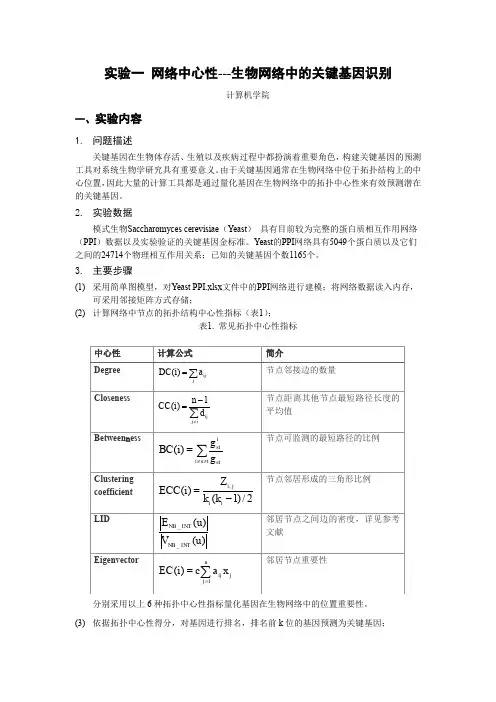
3.主要步骤(1)采用简单图模型，对Yeast PPI.xlsx文件中的PPI网络进行建模；将网络数据读入内存，可采用邻接矩阵方式存储；(2)计算网络中节点的拓扑结构中心性指标（表1）；表1. 常见拓扑中心性指标分别采用以上6种拓扑中心性指标量化基因在生物网络中的位置重要性。

(3)依据拓扑中心性得分，对基因进行排名，排名前k位的基因预测为关键基因；(4) 结果的比较分析：比较6种不同拓扑指标的预测结果。

随着参数k 的不断增大，计算在不同k 值下预测结果的准确率。

二、分析及设计1. 数据预处理首先对拿到的xlxs 格式表格进行预处理，将其转换为csv 合适，以更方便编程使用。

2. 计算网络中节点的拓扑结构中心性指标 (1) Degree 度，节点邻接边的数量，即边集合{a}中包含某个节点的边的个数，由于边的值是0,1，所以degree 公式为：其中i 为待求得某个节点,j 为与i 连接的某个节点，ij a 为节点间的边且有：1 , 0 ij if i j are connecteda otherwise⎧=⎨⎩ (2) Closeness 紧密中心性，定义了单个节点的紧密程度，是节点距离其他节点最短路径长度的平均值。