当前位置：文档之家› 流固耦合简单示例

流固耦合简单示例

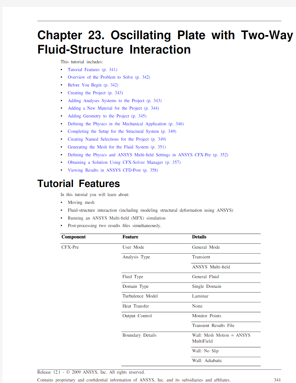
Chapter 23. Oscillating Plate with Two-Way Fluid-Structure Interaction

This tutorial includes:

Tutorial Features (p. 341)?

Overview of the Problem to Solve (p. 342)?

Before You Begin (p. 342)?

Creating the Project (p. 343)?

Adding Analyses Systems to the Project (p. 343)?

Adding a New Material for the Project (p. 344)?

Adding Geometry to the Project (p. 345)?

De?ning the Physics in the Mechanical Application (p. 346)?

Completing the Setup for the Structural System (p. 349)?

Creating Named Selections for the Project (p. 349)?

Generating the Mesh for the Fluid System (p. 351)?

De?ning the Physics and ANSYS Multi-?eld Settings in ANSYS CFX-Pre (p. 352)?

Obtaining a Solution Using CFX-Solver Manager (p. 357)?Viewing Results in ANSYS CFD-Post (p. 358)

Tutorial Features

In this tutorial you will learn about:

Moving mesh ?

Fluid-structure interaction (including modeling structural deformation using ANSYS)?

Running an ANSYS Multi-?eld (MFX) simulation ?Post-processing two results ?les simultaneously.

Details Feature

Component General Mode User Mode

CFX-Pre

Transient

Analysis Type ANSYS Multi-?eld

General Fluid Fluid Type

Single Domain Domain Type

Laminar Turbulence Model

None Heat Transfer

Monitor Points

Output Control Transient Results File

Wall: Mesh Motion = ANSYS

MultiField

Boundary Details Wall: No Slip Wall: Adiabatic

Overview of the Problem to Solve

Details

Feature

Component

Timestep

Transient

Animation

CFD-Post

Plots

Contour

Vector

Overview of the Problem to Solve

This tutorial uses an example of an oscillating plate to demonstrate how to set up and run a simulation involving

two-way Fluid-Structure Interaction (FSI) in ANSYS Workbench. In this tutorial, the structural physics is set up

in the Transient Structural (ANSYS) analysis system and the ?uid physics is set up in Fluid Flow (CFX) analysis

system, but both structural and ?uid physics are solved together under the Solution cell of the Fluid system. Coupling between two analyses systems is required throughout the solution to model the interaction between structural and

?uid systems as time progresses. The framework for the coupling is provided by the ANSYS Multi-?eld solver

using the MFX setup.

The geometry consists of a 2D closed cavity and a thin plate, 1 m high, that is anchored to the bottom of the cavity

as shown below:

An initial pressure of 100 Pa is applied to one side of the thin plate for 0.5 seconds in order to distort it. Once this pressure is released, the plate oscillates backwards and forwards as it attempts to regain its equilibrium (vertical)

position. The surrounding ?uid damps the plate oscillations, thereby decreasing the amplitude of oscillations with time. The CFX solver calculates how the ?uid responds to the motion of the plate, and the ANSYS solver calculates how the plate deforms as a result of both the initial applied pressure and the pressure resulting from the presence

of the ?uid. Coupling between the two solvers is required since the structural deformation affects the ?uid solution, and the ?uid solution affects the structural deformation.

Before You Begin

?Preparing a Working Directory

This tutorial uses the geometry ?le, OscillatingPlate.agdb, for setting up the project. This ?le is located

in /examples, where is the installation directory for ANSYS CFX.

Copy the supplied geometry ?le, OscillatingPlate.agdb, to a directory of your choice. This directory

will be referred to as the working directory in this tutorial.

By working with copy of the geometry ?le in a new directory, you prevent accidental changes to the ?le that

came with your installation.

?Changing the Appearance of ANSYS CFX Applications

If this is the ?rst tutorial you are working with, see Changing the Display Colors (p. 4) for information on

how to change the appearance of ANSYS CFX applications.

Creating the Project

1.Start ANSYS Workbench.

To launch ANSYS Workbench on Windows, click the Start menu, then select All Programs > ANSYS 12.1

> Workbench . To launch ANSYS Workbench on Linux, open a command line interface, type the path to

“runwb2” (for example, “~/ansys_inc/v121/Framework/bin/Linux64/runwb2”), then press Enter .

The Project Schematic appears with an Unsaved Project. By default, ANSYS Workbench is con?gured to

show the Getting Started dialog box that describes basic operations in ANSYS Workbench. Click the [X]

icon to close this dialog box. To turn on or off this dialog box, select Tools > Options from the main menu

and set Project Management > Startup > Show Getting Started Dialog as desired.

2.Select File > Save or click

Save .

A Save As dialog box appears. Select the path to your working directory to store ?les created during this

tutorial. For details, see Preparing a Working Directory .

3.Under File name , type OscillatingPlate and click Save .

The project ?les and their associated folder locations appear under the Files View . To make the Files View

visible, select View > Files from the main menu of ANSYS Workbench.

Adding Analyses Systems to the Project

In ANSYS Workbench, the two-way FSI analysis can be performed by setting up coupled analyses systems,

comprising of a Transient Structural (ANSYS) system and a Fluid Flow (CFX) system as outlined in this section.

1.Expand the Analysis Systems option in the toolbox, located on the left side of the ANSYS Workbench window,

and select the Transient Structural (ANSYS) template. Double-click the template, or drag it onto the Project

Schematic to create a standalone system.

A Transient Structural (ANSYS) system is added to the Project Schematic, with its name selected and ready

to be renamed.

2.Type in the new name, Structural , to replace the selected text. This name will be used while referring to

the Transient Structural (ANSYS) system in this tutorial.

If you missed seeing the selected text, right-click the ?rst cell in the system and select Rename as shown in

the following ?gure. The name will then be selected and ready to change.

3.Now right-click the Setup cell in the Structural system and select Transfer Data to New > Fluid Flow (CFX).

A Fluid Flow system, coupled to the ANSYS system, is added to the Project Schematic.

4.Change the name of this system to Fluid ; this name will be used while referring to the Fluid Flow (CFX)system in this tutorial.

343

Adding a New Material for the Project

For this tutorial, the Solution and Results cells of the Structural system will be removed because they are not used for two-way FSI analysis. This tutorial relies on the solution and result generated in the Fluid system, which you

have already connected to the Structural system.

The following steps outline the removal of these cells from the Structural system:

1.In the Structural system, right-click the Solution cell and select Delete.

2.Click OK on the pop-up message box to con?rm the deletion of the cell with the solution data from the Structural

system.

The Solution and Results cells disappear from the Structural system. The updated project is shown in Figure 23.1,

“Project setup for two-way FSI analysis” (p. 344).

Figure 23.1. Project setup for two-way FSI analysis

3.Now from the main menu, select File > Save to save the project setup.

The Structural and Fluid systems contain various cells and ANSYS Workbench provides visual indications of a

cell's state at any given time via icons on the right side of each cell. In Figure 23.1, “Project setup for two-way FSI analysis” (p. 344), most cells appear with a blue question mark (?), indicating that cells need to be set up before

continuing the analysis. As these cells are set up, the data transfer occurs from top to bottom. See Understanding

States in ANSYS Workbench help for a description of various cell states.

Now the project is ready for further processing. A project with inter-connected systems enables you to perform the analysis by adding a new material, sharing the geometry, setting up the physics in the Structural system, and setting up the physics in the Fluid system. Later, the analysis will be performed in the Fluid system for solving and viewing results.

In Figure 23.1, “Project setup for two-way FSI analysis” (p. 344), the Engineering Data cell appears in an up-to-date state, because a default material de?nition is already available for the project. However, the default material is not used in this tutorial. Thus, the next step in the analysis is to add a new material with properties desired for exhibiting an oscillation under the in?uence of external pressure, as outlined in Overview of the Problem to Solve (p. 342).

The new material can be created using the Engineering Data application in ANSYS Workbench, as described in

the next section.

Adding a New Material for the Project

This section describes how to create a new material named Plate, de?ne its properties suitable for oscillation, and

set it as the default material for the analysis.

1.On the Project Schematic, double-click the Engineering Data cell in the Structural system.

The Outline and Properties windows appear below the Project Schematic.

2.In the Outline Filter window, ensure that Engineering Data is selected.

3.In the Outline of Schematic A2: Engineering Data window, click the empty row at the bottom of the table

to add a new material for the project. Type in the name Plate.

Plate is created and appears with a blue question mark (?), indicating that plate properties need to be de?ned.

4.Now from toolboxes located on the left side of the ANSYS Workbench window, expand the Physical Properties

toolbox. Select Density and drag it onto the cell containing Plate in the Outline of Schematic A2: Engineering

Data window.

Density is added as the plate property in the Properties of Outline Row 4: Plate window, as shown in the

following ?gure.

In the Properties of Outline Row 4: Plate window, set Density to 2550 [kg m^-3].6.Similarly, from the Linear Elastic toolbox, drag Isotropic Elasticity onto Plate in the Outline of Schematic

A2: Engineering Data window.

Isotropic Elasticity is added as the plate property in the Properties of Outline Row 4: Plate window.

7.In the Properties of Outline Row 4: Plate window, expand Isotropic Elasticity by clicking on the plus sign.

Now set Young's Modulus to 2.5e06 [Pa] and Poisson's Ratio to 0.35.

Now the desired plate data is created and will be available to remaining cells in the Structural system. The next step is to set Plate as the default material for the analysis as outlined below:

In the Outline of Schematic A2: Engineering Data window, under Material , right-click Plate to open the shortcut menu.2.

In the shortcut menu, select Default Solid Material For Model .3.Now from the main menu, select File > Save to save material settings to the project.

Now from the ANSYS Workbench toolbar, click Return to Project to close the Engineering Data workspace and

return to the Project Schematic. The Outline and Properties windows disappear.

Adding Geometry to the Project

This section describes how to add geometry by importing an existing DesignModeler ?le and unsuppress geometry parts in order to make them available for subsequent cells in the Structural and Fluid systems.

345

De?ning the Physics in the Mechanical Application

1.On Project Schematic, right-click the Geometry cell in the Structural system and select Import Geometry >

Browse. In the Open dialog box, select OscillatingPlate.agdb from your working directory. For

details, see Preparing a Working Directory.

The geometry is included in the project and Geometry cells appear in an up-to-date state in both the Structural

and Fluid systems.

2.In the Structural system, double-click the Geometry cell to edit the geometry using DesignModeler.

Note

The Geometry cell in the Fluid system cannot be edited because it is being shared with the Geometry

cell in the Structural system.

In DesignModeler, the Tree Outline contains two bodies, Fluid body and Solid body, under the branch named 2 , as shown in the following ?gure.

Parts, 2 Bodies

a body is suppressed in DesignModeler, its model data is not exported to subsequent cells in the analysis systems.

For this tutorial, all bodies will be unsuppressed in DesignModeler so that all geometry data is transferred to the

subsequent cells in the Structural and Fluid systems. Later in the tutorial, the Solid and Fluid body will be selectively suppressed in the Structural and Fluid systems, respectively, before generating an appropriate structural or ?uid

mesh.

1.In the Tree Outline, right-click the Fluid and select Unsuppress Body.

The status of the Fluid body changes to a green check mark.

2.In the Tree Outline, select the branch named 2 Parts, 2 Bodies, both the Fluid and Solid bodies should be

visible in the Graphics window. Click Zoom to Fit to view the entire model in the Graphics window.

This ?nishes the geometry setup for the project. Save these changes by selecting File > Save Project from the main menu, and select File > Close DesignModeler to return to the Project Schematic.

Now the updated geometry is available for both the Structural and Fluid systems.

Defining the Physics in the Mechanical Application This section describes the step-by-step de?nition of the structural physics in the following sections:

?Generating the Mesh for the Structural System (p. 347)

?Assigning the Material to Geometry (p. 347)

?Basic Analysis Settings (p. 347)

?Inserting Loads (p. 347)

Generating the Mesh for the Structural System

This section describes how to generate mesh for the Structural system.

1.On the Project Schematic, double-click the Model cell in the Structural system.

The Mechanical application appears.

2.In the Mechanical application, expand Project > Model > Geometry in the tree view.

Two geometries, Solid and Fluid, appear in the tree view. Click

Zoom to Fit

to view the entire model in

the Graphics window.For the Structural system, the mesh needs to be generated from the Solid body. As such, the Fluid body will

be suppressed before the mesh generation operation.

3.Right-click the Fluid geometry and select Suppress Body from the shortcut menu.

The Fluid body becomes suppressed and its status changes to an x mark. Click Zoom to Fit

to re-size the

model suitable for viewing in the Graphics window.

4.In the tree view, right-click Mesh and select Generate Mesh from the shortcut menu.

The hex mesh is generated.Assigning the Material to Geometry

1.In the Mechanical application, expand Project > Model > Geometry in the tree view and select Solid .

The details of Solid appear in the Details view below the Outline tree view.

2.In the Details view, ensure Material > Assignment is set to Plate . Otherwise, click on the material name

and use the arrow that appears next to the material name to make appropriate changes.

Basic Analysis Settings

This section outlines the steps to set up an ANSYS Multi-?eld run using the transient mechanical analysis, with a

timestep of 0.1 s and a time duration of 5 s. For the given material properties of the plate, the time duration is chosen to allow the plate to oscillate just a few times, and the timestep is chosen to resolve those oscillations to a reasonable degree.

1.In the Mechanical application, expand Project > Model > Transient in the tree view and select Analysis

Settings .

The details of Analysis Settings appear in the Details view below the Outline tree view.

2.In the Details view, specify the following settings under Step Controls :Note

Do not type in units while entering data for the time settings, Time Step and Step End Time .

Set Auto Time Stepping to Off ?

Set Time Step to 0.1?Set Step End Time to 5.

Inserting Loads

The loads applied for the ?nite element analysis are equivalent to the boundary conditions in ?uid analysis. In this section, you will set a ?xed support, a ?uid-solid interface, and a pressure load. On the surfaces of the plate that lie coincident with the symmetry planes, no loads are set. As a result, the default of an unconstrained condition will

be applied on these surfaces. For this particular application, this is a reasonable approximation of the frictionless support that would otherwise be applied.

347

Inserting Loads

Fixed Support

The ?xed support is required to hold the bottom of the thin plate in place.

1.In the Mechanical application, expand Project > Model and right-click Transient in the tree view and select

Insert > Fixed Support from the shortcut menu.

2.Rotate the geometry using the Rotate button so that the bottom (low-y) face of the solid is visible, then

select Face and click the low-y face.

That face should be highlighted to indicate the selection.

3.In the Details view, click Apply to set the ?xed support.

The text next to the Geometry setting changes to 1 Face.

If the Apply button is not visible, select Fixed Support in the tree view and, in the Details view, click on the

text next to the Geometry setting to make the Apply button re-appear.

Fluid-Solid Interface

The ?uid-solid interface de?nes the interface between the ?uid in the Fluid system and the solid in the Structural

system. This interface is de?ned on regions in the structural model. Data is exchanged across this interface during the execution of the simulation.

1.In the Mechanical application, expand Project > Model and right-click Transient in the tree view and select

Insert > Fluid Solid Interface from the shortcut menu.

https://www.doczj.com/doc/ef1112549.html,ing the same face-selection procedure described earlier in Fixed Support (p. 348), select the three faces of

the geometry that form the interface between the structural model and the ?uid model (low-x, high-y and high-x

faces) by holding down Ctrl to select multiple faces.

Note that this load (?uid-solid interface) is automatically given an interface number of 1.

Pressure Load

The pressure load provides the initial additional pressure of 100 [Pa] for the ?rst 0.5 seconds of the simulation.

It is de?ned using a step function.

1.In the Mechanical application, expand Project > Model and right-click Transient in the tree view and select

Insert > Pressure from the shortcut menu.

2.Select the low-x face for Geometry and click Apply.

3.In the Details view, select Magnitude, and using the arrow that appears, select Tabular data.

4.Under Tabular Data at the bottom right of the Mechanical application window, set a pressure of 100 in the

table row corresponding to a time of 0.

Note

Do not type in units while entering the tabular data. The units for time and pressure in this table

are the global units of [s] and [Pa], respectively.

5.You now need to add two new rows to the table. This can be done by typing the new time and pressure data

into the empty row at the bottom of the table, and rows will be automatically re-ordered based on the time

value. Enter a pressure of 100 for a time value of 0.499, and a pressure of 0 for a time value of 0.5 Array

This gives a step function for pressure that can be seen in the chart to the left of the table.

The settings for structural physics are now complete. Save these settings by selecting File > Save Project from the main menu, and select File > Close Mechanical to close the Mechanical application and return to the Project

Schematic.

Completing the Setup for the Structural System

On the Project Schematic, the Setup cell in the Structural system appears in an update-required state. This section describes how to update the Setup cell in the Structural system.

1.In the Structural system, right-click the Setup cell and select Update from the shortcut menu.

The status of the Setup cell changes to up-to-date . Now all cells in the Structural system should appear in an

up-to-date state.

2.Now from the main menu, select File > Save to save the project.

This completes the setup for the Structural system. In the next section, the Fluid system will be set up.

As the Geometry cell is already up to date for both the Solid and Fluid systems, the next section begins with the

setup of Mesh cell. Before generating mesh for the Fluid system, geometry faces will be grouped by creating Named Selections in the Meshing application as discussed in the next section.

Creating Named Selections for the Project

This section describes how to group geometry faces using Named Selections in the Meshing application. Later,

when a mesh is generated from the model containing Named Selections, the grouped geometry faces are retained

in the mesh and are accessible from within ANSYS CFX in the form of Regions .

On the Project Schematic, right-click the Mesh cell in the Fluid system and select Edit to open the model in the Meshing application.2.Ensure that the Meshing application is open. If you ?nd that CFX-Mesh is open, then close it and return to the

Meshing application by selecting File > Close CFX-Mesh from the CFX-Mesh's main menu.

If CFX-Mesh opens initially, then a default mesh method, CFX-Mesh Method, is added to the model in the

Meshing application. For this tutorial, it is required that you remove any existing mesh methods from the

model; the instructions to do this will be revisited later in Generating the Mesh for the Fluid System (p. 351).Note

If you have con?gured the Meshing application to use CFX-Mesh as the default mesh method, then

upon editing the Mesh cell for the ?rst time, the Meshing application will load initially and will be

replaced by CFX-Mesh automatically. However, if you are editing the Mesh cell in a subsequent

attempt, then only the Meshing application opens.

Typically, the Meshing application and CFX-Mesh can be identi?ed from their tree views, as shown in the

following ?gure. In the Meshing application, Project appears as the top-level item in the tree view, whereas

Model is the top-level item in the tree view of CFX-Mesh. Also, notice differences in names of the tree view

windows, Outline versus Tree View .

349

Release 12.1 - ? 2009 ANSYS, Inc. All rights reserved.Contains proprietary and con?dential information of ANSYS, Inc. and its subsidiaries and af?https://www.doczj.com/doc/ef1112549.html,pleting the Setup for the Structural System

Creating Named Selections for the Project

Now create a Named Selection, Sym1, by selecting the high-z face of the Fluid body, as outlined below. The

procedure to create the Named Selections is outlined below:

1.In the Meshing application, expand Project > Model > Geometry in the tree view.

Two items, Fluid body and Solid body, appear under the Geometry tree object.

2.Right-click the Solid body and select Suppress Body from the shortcut menu.

The Solid body becomes suppressed and its status changes to an x mark.

3.In the tree view, right-click the Fluid body and select Create Selection Group from the shortcut menu.

The Selection Name dialog box appears.

4.In the Selection Name dialog box, type in Sym1 for the name of the selection group.

A Named Selections branch is added to the tree view.

5.Expand the Named Selections branch and select Sym1.

The details of Sym1 appear in the Details view below the tree view. Notice Scope > Geometry is set to 1

Body.

6.In the Details view, click 1 Body to make the Apply button appear.

7.In the graphics window, rotate the geometry using the Rotate button so that the high-z face of the geometry

is visible, then select Face and click the high-z face.

That face should be highlighted to indicate the selection.

8.In the Details view, Click Apply to set the selected face.

The Geometry setting changes to 1 Face.

Similarly, create another Named Selection, Sym2 by selecting the low-z face of the Fluid body, as outlined below:

1.In the tree view, right-click the Fluid body and select Create Selection Group from the shortcut menu.

The Selection Name dialog box appears.

2.In the Selection Name dialog box, type in Sym2 for the name of the selection group.

Sym2 is added to the Named Selection branch in the tree view.

3.Select Sym2 in the tree view.

The details of Sym2 appear in the Details view below the tree view. Notice Scope > Geometry is set to 1

Body.

In the Details view, click 1 Body to make the Apply button appear.5.In the graphics window, rotate the geometry using the Rotate

button so that the low-z face of the geometry

is visible, then select Face and click the low-z face.That face should be highlighted to indicate the selection.

6.In the Details view, Click Apply to set the selected face.

The Geometry setting changes to 1 Face .

This ?nishes the creation of Named Selections on the Fluid body. Do not close the Meshing application yet, the

tutorial continues to set up mesh settings and generate mesh for the Fluid system in the next section.

Generating the Mesh for the Fluid System

1.In the Meshing application, expand Project > Model > Geometry in the tree view.

Two geometries, Solid and Fluid, appear under Geometry.

For the Fluid system, the mesh needs to be generated from the Fluid body, thus the Solid body will be suppressed.

The mesh for the Solid body has already been generated earlier in this tutorial.

2.In the tree view, expand Project > Model > Mesh and ensure that the Mesh branch does not contain any other

objects. Otherwise, right-click such objects and select Delete from the shortcut menu.

Typically, if you have con?gured the Meshing application to use CFX-Mesh for meshing, then CFX-Mesh

Method is added as a default mesh method under the Mesh branch. In such a case, right-click CFX-Mesh

Method and select Delete to remove it from the Mesh branch.

3.Ensure Mesh is selected in the tree view.

The details of Mesh appear in the Details view below the Outline tree view.

4.In the Details view, set Sizing > Relevance Center to Medium .

This controls the grid resolution of the mesh.

5.Now in the tree view, right-click Mesh and select Insert > Method from the shortcut menu.

Method is added to Mesh branch in the tree view. In the details view, Apply and Cancel buttons appear next

to the Geometry Setting.

Click anywhere on the geometry in the viewer to select the Fluid body.7.In the details view, click on the Apply button next to the Geometry setting.

Notice Scope > Geometry is now set to 1 Body .

8.In the details view, set the following mesh settings in the following order:

Set De?nition > Method to Sweep .2.

Set Free Face Mesh Type to All Tri .3.

Set Sweep Num Divs = 1.9.Now in the tree view, right-click Mesh and select Generate Mesh from the shortcut menu.

The mesh is generated.

10.This ?nishes the mesh generation for the Fluid system. From the main menu, select File > Save Project to

save these changes to the project, and select File > Close Meshing to return to the Project Schematic.

On the Project Schematic, the Mesh cell in the Fluid system appears in an update-required state.

?Right-click the Mesh cell and select Update from the shortcut menu.

Updating of the Meshing cell is required as opening ANSYS CFX-Pre, from the Setup cell, with an out-of-date Meshing cell can potentially corrupt the project.

351

Defining the Physics and ANSYS Multi-field Settings in ANSYS CFX-Pre

This section describes the step-by-step de?nition of the ?ow physics and ANSYS Multi-?eld settings in the following sections:

?Setting the Analysis Type (p. 352)

?Creating the Fluid (p. 353)

?Creating the Domain (p. 353)

?Creating the Boundaries (p. 354)

?Setting Initial Values (p. 355)

?Setting Solver Control (p. 355)

?Setting Output Control (p. 356)

Setting the Analysis Type

A transient ANSYS Multi-?eld run executes as a series of timesteps. In ANSYS CFX-Pre, the Analysis Type tab

is used to enable both an ANSYS Multi-?eld run and to specify time-related settings for the coupled solver run.

ANSYS CFX-Pre reads the ANSYS input ?le, which is automatically passed by ANSYS Workbench, in order to

determine ?uid-solid interfaces created in the Mechanical application.

1.On the Project Schematic, double-click the Setup cell in the Fluid system to launch the ANSYS CFX-Pre

application.

2.In ANSYS CFX-Pre, click

Analysis Type.

3.Apply the following settings:

Value

Setting

Tab

ANSYS MultiField

External Solver Coupling > Option

Basic Settings

Total Time

Coupling Time Control > Coupling Time Duration >

Option

5 [s]

Coupling Time Control > Coupling Time Duration > Total

Time

Timesteps

Coupling Time Control > Coupling Time Steps > Option

0.1 [s]

Coupling Time Control > Coupling Time Steps >

Timesteps

Transient

Analysis Type > Option

Coupling Time

Duration a

Analysis Type > Time Duration > Option

Coupling Timesteps a

Analysis Type > Time Steps > Option

Coupling Initial Time

Analysis Type > Initial Time > Option

a Once the timesteps and time duration are speci?ed for the ANSYS Multi-?eld run (coupling run), CFX automatically picks up these

settings and it is not possible to set the timestep and time duration independently. Hence the only option available for Time Duration is

Coupling Time Duration, and similarly for the related settings Time Step and Initial Time.

4.Click OK.

De?ning the Physics and ANSYS Multi-?eld Settings in ANSYS CFX-Pre

Creating the Fluid

A custom ?uid is created with user-speci?ed properties.

Click Material and set the name of the material to Fluid .2.Apply the following settings:

Value Setting Tab

Pure Substance Option

Basic Settings (Selected)Thermodynamic State

Liquid Thermodynamic State > Thermodynamic State

1 [kg kmol^-1] a Equation of State > Molar Mass

Material

Properties 1 [kg m^-3] b Equation of State > Density

(Selected)Transport Properties > Dynamic Viscosity

0.2 [Pa s] b Transport Properties > Dynamic Viscosity > Dynamic

Viscosity

a The molar mass is not used for this tutorial setup and has been set only for the completeness of the ?uid property.

The ?uid properties are chosen to ensure that the plate generates a reasonable amplitude of vibration that doesn't decay too fast under the in?uence of ?uid.3.Click OK .

Creating the Domain

In order to allow ANSYS Solver to communicate mesh displacements to CFX-Solver, mesh motion must be activated in CFX.

Edit Case Options > General in the Outline tree view and ensure that Automatic Default Domain is turned on. A domain named Default Domain should now appear under the Simulation branch.2.Double-click Default Domain and apply the following settings

Value Setting Tab

Fluid 1Fluid and Particle De?nitions

Basic Settings Fluid Fluid and Particle De?nitions > Fluid 1 >

Material

1 [atm] a Domain Models > Pressure > Reference

Pressure

Regions of Motion Speci?ed Domain Models > Mesh Deformation >

Option

None Heat Transfer > Option

Fluid Models None (Laminar)Turbulence > Option

a The reference pressure has no effect on this simulation so leave it as the default.

3.Click OK .

353

Creating the Boundaries

In addition to the symmetry conditions, this tutorial requires boundary conditions for an external boundary resulting from the ?uid-solid interface as outlined below:

?Fluid Solid External Boundary (p. 354)

?Symmetry Boundaries (p. 354)

Fluid Solid External Boundary

The interface between ANSYS and CFX is considered as an external boundary in CFX-Solver with its mesh

displacement being de?ned by the ANSYS Multi-?eld coupling process. This section outlines the steps to create a Boundary Type for CFX and specify a matching ANSYS interface. This speci?cation sets up CFX-Solver to pass forces to ANSYS solver on this boundary, and to receive the mesh displacement calculations from the ANSYS

solver under the effect of forces from CFX or other de?ned loads.

When an ANSYS Multi-?eld speci?cation is being made in CFX-Pre, it is necessary to provide the name and

number of the matching Fluid Solid Interface that was created in the Mechanical application, in the form of

FSIN_#, where # is the interface number that was created in the Mechanical application. Since the interface number in the Mechanical application was 1, the name in question is FSIN_1. (If the interface number had been 2, then

the name would have been FSIN_2, and so on.)

On this boundary, CFX will send ANSYS the forces on the interface, and ANSYS will send back the total mesh

displacement it calculates given the forces passed from CFX and the other de?ned loads.

1.Create a new boundary named Interface.

2.Apply the following settings

Tab

Value

Setting

Basic Settings

Wall

Boundary Type

Location

F33.30, F34.30, F35.30a Boundary Details

ANSYS MultiField

Mesh Motion > Option

Mesh Motion > Receive From ANSYS

Total Mesh Displacement

Mesh Motion > ANSYS Interface

FSIN_1

Mesh Motion > Send to ANSYS

Total Force

a Alternatively, the geometry faces could be grouped together and named using Named Selections in the Meshing application.

3.Click OK.

Symmetry Boundaries

Since a 2D representation of the ?ow ?eld is being modeled (using a 3D mesh with one element thickness in the Z direction) symmetry boundaries will be created on the low and high Z 2D regions of the mesh.

1.Create a new boundary named Sym1.

2.Apply the following settings

Setting

Value

Tab

Basic Settings

Symmetry

Boundary Type

Sym1

Location

3.Click OK.

4.Create a new boundary named Sym2.

5.Apply the following settings

Value Setting Tab

Symmetry Boundary Type

Basic Settings Sym2

Location

6.Click OK .Setting Initial Values

Since a transient simulation is being modeled, initial values are required for all variables.

Click Global Initialization .

2.Apply the following settings:

Value Setting Tab

0 [m s^-1] a Initial Conditions > Cartesian Velocity

Components > U

Global Settings 0 [m s^-1] a Initial Conditions > Cartesian Velocity

Components > V

0 [m s^-1] a Initial Conditions > Cartesian Velocity

Components > W 0 [Pa] a

Initial Conditions > Static Pressure > Relative Pressure

a These settings ensure that the ?uid is at rest initially, and the ?ow is generated by the initial motion of the plate.

3.Click OK .

Setting Solver Control

Various ANSYS Multi-?eld settings are contained under Solver Control under the External Coupling tab. Most of these settings do not need to be changed for this simulation.

Within each timestep, a series of coupling or stagger iterations are performed to ensure that CFX-Solver, the Mechanical application and the data exchanged between the two solvers are all consistent. Within each stagger iteration, the Mechanical application and CFX-Solver both run once each, but which one runs ?rst is a user-speci?able setting. In general, it is slightly more ef?cient to choose the solver that drives the simulation to run ?rst. In this case, the simulation is being driven by the initial pressure applied in the Mechanical application, so the Mechanical application is set to solve before CFX-Solver within each stagger iteration.

Click

Solver Control .2.Apply the following settings:

Value Setting Tab

Second Order Backward

Euler

Transient Scheme > Option Basic Settings 3

Convergence Control > Max. Coeff. Loops Before CFX Fields

Coupling Step Control > Solution Sequence Control > Solve ANSYS Fields External Coupling 355

Value Setting

Tab FZ Coupling Data Transfer Control > Ansys

Variable

(Selected)Coupling Data Transfer Control > Ansys

Variable > FZ

(Selected)Coupling Data Transfer Control > Ansys

Variable > FZ > Convergence Target

1a Coupling Data Transfer Control > Ansys

Variable > FZ > Convergence Target >

Convergence Target

UZ Coupling Data Transfer Control > Ansys

Variable

(Selected)Coupling Data Transfer Control > Ansys

Variable > UZ

(Selected)Coupling Data Transfer Control > Ansys

Variable > UZ > Convergence Target

1 a Coupling Data Transfer Control > Ansys

Variable > UZ > Convergence Target >

Convergence Target

a Since the Z component of both the force (FZ) and resultant displacement (UZ) are negligible for this 2-D case, their convergence targets are set to large values in order to negate their in?uence when determining load convergence.

3.Click OK .

Setting Output Control

This step sets up transient results ?les to be written at set intervals.

Click Output Control .2.

Click the Trn Results tab.3.

In the Transient Results tree view, click Add new item , accept the default name and click OK .4.Apply the following settings:

Value Setting

Selected Variables Option

Pressure, Total Mesh Displacement, Velocity Output Variable List

Every Coupling Step a Output Frequency > Option

a This setting writes a transient results ?le every multi-?eld timestep.

Click the Monitor tab.6.

Select Monitor Options .7.Under Monitor Points and Expressions :

Click Add new item and accept the default name.2.Set Option to Cartesian Coordinates .

356Contains proprietary and con?dential information of ANSYS, Inc. and its subsidiaries and af?liates.

Setting Output Control

Set Output Variables List to Total Mesh Displacement X .4.Set Cartesian Coordinates to [0, 1, 0].

This monitor point measures the x-component of the total mesh displacement at the top of the plate.

8.Click OK .

The settings for ?uid physics are now complete. From the main menu, select File > Save Project to save these changes to the project, and select File > Quit to close ANSYS CFX-Pre and return to the Project Schematic.Obtaining a Solution Using CFX-Solver Manager

The execution of an ANSYS Multi-?eld simulation requires both the CFX and ANSYS solvers to be running and communicating with each other. This section outlines the steps to launch both solvers and monitor the output using ANSYS CFX-Solver Manager.

1.On the Project Schematic, double-click the Solution cell in the Fluid system to launch the ANSYS CFX-Solver

Manager application.

ANSYS Workbench generates the CFX-Solver input ?le and passes it to ANSYS CFX-Solver Manager.

2.In ANSYS CFX-Solver Manager, ensure that De?ne Run dialog box is displayed.

On the De?ne Run dialog box, Solver Input File is set automatically by ANSYS Workbench. The CFX-Solver input ?le contains settings for an ANSYS Multi-?eld simulation, thus MultiField tab appears on the De?ne Run dialog box.

On the MultiField tab, ANSYS Input File is set automatically by ANSYS Workbench.4.

On UNIX systems, you may need to manually specify where the ANSYS installation is if it is not in the default location. In this case, you must provide the path to the v121/ansys directory.5.Click Start Run .Note

On the Run De?nition tab, the Initialization Option ?eld is set to Current Solution Data (if possible),

its default setting. These runs use the results from any previous solution run as initial values for a

subsequent update. This may not be desirable when restarting transient runs, which typically need to

start from the initial conditions speci?ed in the Setup cell. See Properties View (p. 54) in the ANSYS

CFX Introduction for more details.

The run begins by some initial processing of the ANSYS Multi-?eld input which results in the creation of a ?le containing the necessary multi-?eld commands for ANSYS, and then the ANSYS Solver is started. The CFX Solver is then started in such a way that it knows how to communicate with the ANSYS Solver.

After the run is under way, two new plots appear in ANSYS CFX-Solver Manager:

?ANSYS Field Solver (Structural)This plot is produced only when the solid physics is set to use large

displacements or when other non-linear analyses are performed. It shows convergence of the ANSYS Solver.Full details of the quantities are described in the ANSYS user documentation. In general, the CRIT quantities are the convergence criteria for each relevant variable, and the L2 quantities represent the L2 Norm of the

relevant variable. For convergence, the L2 Norm should be below the criteria. The x-axis of the plot is the

cumulative iteration number for ANSYS, which does not correspond to either timesteps or stagger iterations.Several ANSYS iterations will be performed for each timestep, depending on how quickly ANSYS converges.You will usually see a somewhat spiky plot, as each quantity will be unconverged at the start of each timestep,and then convergence will improve.

ANSYS Interface Loads (Structural)This plot shows the convergence for each quantity that is part of the data exchanged between the CFX and ANSYS Solvers. Six lines appear, corresponding to three force components (FX, FY , and FZ) and three displacement components (UX, UY , and UZ). Each quantity is converged when the plot shows a negative value. The x-axis of the plot corresponds to the cumulative number of stagger iterations (coupling iterations) and there are several of these for every timestep. Again, a spiky plot is expected as the quantities will not be converged at the start of a timestep.357

Viewing Results in ANSYS CFD-Post

The ANSYS out ?le is displayed in ANSYS CFX-Solver Manager as an extra tab. Similar to the CFX out ?le, this is a text ?le recording output from ANSYS as the solution progresses.

1.Click the User Points tab and watch how the top of the plate displaces as the solution develops.

When the solver run has ?nished, a completion message appears in a dialog box.

2.Click OK.

From the main menu, select File > Quit to close ANSYS CFX-Solver Manager and return to the Project Schematic. Viewing Results in ANSYS CFD-Post

On the Project Schematic, double-click the Results cell in the Fluid system to launch the ANSYS CFD-Post

application.

Being an ANSYS Multi-?eld run, both the CFX and ANSYS results ?les will be opened up in CFD-Post. Plotting Results on the Solid

When ANSYS CFD-Post reads an ANSYS results ?le, all the ANSYS variables are available to plot on the solid,

including stresses and strains. The mesh regions available for plots by default are limited to the full boundary of

the solid, plus certain named regions which are automatically created when particular types of load are added in

Simulation. For example, any Fluid-Solid Interface will have a corresponding mesh region with a name such as

FSIN 1. In this case, there is also a named region corresponding to the location of the ?xed support, but in general pressure loads do not result in a named region.

You can add extra mesh regions for plotting by creating named selections in Simulation - see the Simulation product documentation for more details. Note that the named selection must have a name which contains only English letters, numbers and underscores for the named mesh region to be successfully created.

Note that when ANSYS CFD-Post loads an ANSYS results ?le, the true global range for each variable is not

automatically calculated, as this would add a substantial amount of time depending on how long it takes to load

such a ?le (you can turn on this calculation using Edit > Options and using the Pre-calculate variable global

ranges setting under CFD-Post > Files). When the global range is ?rst used for plotting a variable, it is calculated as the range within the current timestep. As subsequent timesteps are loaded into CFD-Post, the Global Range is

extended each time variable values are found outside the previous Global Range.

1.Turn on the visibility of Default Boundary (under ANSYS at 5s > Default Domain).

2.Right-click a blank area in the viewer and select Prede?ned Camera > View Towards +Z. Zoom into the

plate to see it clearly.

3.Apply the following settings to Default Boundary:

Tab

Value

Setting

Color

Mode

Variable

V on Mises Stress

Variable

4.Click Apply.

5.Select Tools > Timestep Selector from the task bar to open the Timestep Selector dialog box. Notice that a

separate list of timesteps is available for each results ?le loaded, although for this case the lists are the same.

By default, Sync Cases is set to By Time Value which means that each time you change the timestep for

one results ?le, CFD-Post will automatically load the results corresponding to the same time value for all other

results ?les.

6.Set Match to Nearest Available.

7.Change to a time value of 1 [s] and click Apply.

The corresponding transient results are loaded and you can see the mesh move in both the CFX and ANSYS regions.

1.Turn off the visibility of Default Boundary (under ANSYS at 1s > Default Domain).

Create a contour plot, set Locations to ANSYS > Default Boundary and Fluid > Sym2, and set Variable to Total Mesh Displacement . Click Apply https://www.doczj.com/doc/ef1112549.html,ing the timestep selector, load time value 0.8 [s] (which is where the maximum total mesh displacement

occurs).

This veri?es that the contours of Total Mesh Displacement are continuous through both the ANSYS and CFX regions.

Many FSI cases will have only relatively small mesh displacements, which can make visualization of the mesh displacement dif?cult. ANSYS CFD-Post allows you to visually magnify the mesh deformation for ease of viewing such displacements. Although it is not strictly necessary for this case, which has mesh displacements which are easily visible unmagni?ed, this is illustrated by the next few instructions.

Using the timestep selector, load time value 0.1 [s] (which has a much smaller mesh displacement than the currently loaded timestep).2.Place the mouse over somewhere in the viewer where the background color is showing. Right-click and select

Deformation > Auto . Notice that the mesh displacements are now exaggerated. The Auto setting is calculated to make the largest mesh displacement a ?xed percentage of the domain size.

To return the deformations to their true scale, right-click and select Deformation > True Scale .Creating an Animation

Using the Timestep Selector dialog box, ensure the time value of 0.1 [s] is loaded.2.

Turn off the visibility of Contour 1.3.

Turn on the visibility of Sym2.4.Apply the following settings to Sym2.

Value Setting Tab

Variable Mode

Color Pressure

Variable

Click Apply .6.

Create a vector plot, set Locations to Sym1 and leave Variable set to Velocity . Set Color to be Constant and choose black. Click Apply .7.

Turn on the visibility of Default Boundary (under ANSYS at 0.1s > Default Domain ), and set Color to a constant blue.8.Click Animation .The Animation dialog box appears.

9.Select Keyframe Animation .

10.In the Animation dialog box:

Click

New to create KeyframeNo1.2.

Highlight KeyframeNo1, then change # of Frames to 48.3.

Load the last timestep (50) using the timestep selector.4.Click

New to create KeyframeNo2.

The # of Frames parameter has no effect for the last keyframe, so leave it at the default value.

Select Save Movie .6.

Set Format to MPEG1.7.Click Browse next to Save Movie to set a path and ?le name for the movie ?le.

359

Creating an Animation

If the ?le path is not given, the ?le will be saved in the directory from which CFD-Post was launched.

8.Click Save.

The movie ?le name (including path) will be set, but the movie will not be created yet.

9.If frame 1 is not loaded (shown in the F: text box in the middle of the Animation dialog box), click To

Beginning to load it.

10.Click Play the animation.

The movie will be created as the animation proceeds. This will be slow, since a timestep must be loaded

and objects must be created for each frame. To view the movie ?le, you need to use a viewer that supports

the MPEG format.

11.Save the results by selecting File > Save Project from the main menu.

When you are ?nished viewing results in ANSYS CFD-Post, return to the Project Schematic and select File > Exit to exit from ANSYS Workbench.