Performance Evaluation of Software Architectures (1998)

Architectural UnificationRalph Melton and David Garlan*School of Computer ScienceCarnegie Mellon UniversityPittsburgh PA 15213{ralph,garlan}@Phone: (412) 268-7673Fax: (412) 268-557631 January 1997Submitted For Publication, January 1997AbstractMany software designs are produced by combining and elaborating existing architectural design frag-ments. These fragments may be design patterns, partially thought-out ideas, or portions of some previ-ously-developed system design. To provide mechanized support for this activity it is necessary to have aprecise characterization of when and how two or more architectural fragments can be combined. In thispaper we describe extensions to notations for software architecture to represent incomplete design frag-ments, and algorithms for combining fragments in a process analogous to unification in logic.1. IntroductionSoftware architecture is increasingly recognized as an important level of design for software systems. At this design level systems are usually represented as a set of coarse-grained interacting components such as databases, clients, servers, filters, blackboards [GP95, GS93, PW92]. Architectural design describes complex systems at a sufficiently high level of abstraction that their conceptual integrity and other key system properties can be clearly understood early in the design cycle.One of the central benefits of architectural design is support for design reuse. Many systems are built by combining and elaborating existing architectural design fragments [BJ94, BMR+96]. These fragments may be design patterns, partially thought-out ideas, or portions of some previously-developed system design.Currently the practice of reusing architectural fragments has a weak engineering basis. Architectural design frag-ments are usually represented informally and the principles by which partial designs are combined are informal and ad hoc. In particular, given an architectural design fragment it is typically not clear either (a) what aspects of that fragment must be filled in to complete the design, or (b) how to determine whether a given context can satisfy its requirements.USAF, and the Advanced Research Projects Agency (ARPA) under grants F33615-93-1-1330 and N66001-95-C-8623; and by National Science Foundation Grant CCR-9357792. Views and conclusions contained in this document are those of the authors and should not be interpreted as representing the official policies, either expressed or implied, of Wright Laboratory, the US Department of Defense, the United States Government, or the National Science Foundation. The US Government is authorized to reproduce and distribute reprints for Government purposes, notwithstanding any copyright notation thereon.Recently, considerable progress has been made in developing ways to represent software architectures. A number of architectural description languages have been developed, together with tools for manipulating those descriptions, for-mally analyzing them, and storing reusable architectural elements [GAO94, MORT96, LAK+95, MQR95, SDK+95, AG94].While the ability to formally represent architectural designs is a necessary first step, notations and tools for architec-tural representation do not by themselves solve the problems of combining architectural design fragments. First, these notations usually lack any means for characterizing “partiality” in architectural design—that is, explicit identification of missing parts and context requirement. Second, they do not provide effective criteria or mechanisms for combining several fragments into a single coherent design.In this paper we attempt to remedy the situation. First, building on standard representational schemes for software architecture, we show how partial designs can be characterized using architectural placeholders. Second, building on theoretical underpinnings from unification in logic, we provide an algorithm for combining multiple such fragments. The underlying ideas behind our approach are straightforward: Placeholders in an architectural design serve as vari-ables in an architectural expression. Legal combination of several such “expressions” is determined by a form of uni-fication that matches variables to instances. However, as we will show, the domain of architectural representations raises a number of challenges that make the naive application of the traditional unification algorithm difficult (if not impossible). We then show how those challenges can be met by extending the algorithm in several significant ways.2. Related WorkThree areas of research are closely related to this work: software architecture, reuse, and logic.2.1. Software ArchitectureWithin the emerging field of software architecture, two related subareas are architectural description languages (ADLs) and architecture-based reuse.Architecture Description LanguagesA large number of ADLs have been proposed (at last count over a dozen). While these languages differ from each other in many significant ways, virtually all share a common view that a software system’s architecture describes the system’s structure as a hierarchical configuration of interacting components. Beyond this, different ADLs typically add flesh to the structural skeleton by allowing additional semantic information that characterizes such things as abstract behavior, implementation choices, and extra-functional behavior (performance, space requirements, etc.) Our work builds on architecture description languages by adopting their common structural basis (detailed in Section 4). Auxiliary information is handled in our framework by viewing that information as residing as attributes of the architectural structure. (The same approach is taken by a number of other languages, including, Aesop, and UniCon.) In this way our results are largely ADL-neutral: to the extent that an existing ADL adopts our generic structural basis for architectural representation, our results will apply. However, as we will see our work also extends the usual archi-tectural representation schemes, by introducing an explicit notion of a placeholder and mechanisms for filling those placeholders.Architecture-based ReuseResearch in software architecture has focused primarily on two aspects of reuse.•Code: A number of systems (such as GenV oca [BO92] and UniCon [SDK+95] provide high-level compil-ers for certain classes of software architecture. These support reuse of implementations, primarily byexploiting shared implementation structures for some class or domain of systems. However, unlike our work they are less concerned with general mechanisms for reuse of architectures themselves.•Style: Some systems (such as Aesop [GAO94] and Wright [AG94]) support the definition of families of architecture that adopt a common set of design constraints - sometimes called an architecture “style”. For systems within such a family it is often possible to provide (and thereby reuse) specialized analysis tools, code generators, and design guidance. Styles typically prescribe general rules for architecture (such as a specialized design vocabulary and constraints on how the elements are composed). This differs from the work described here, which focuses on reuse of architectural fragments.2.2. ReuseArchitecture aside, the general area of reuse has been an active research area for many years. Historically most of that work has focused on code-level reuse, with an emphasis on representation, retrieval, and adaptation of implementa-tions.More recently, work on design patterns has raised the level of concern to design reuse. In particular, design patterns have been extremely successful in capturing idioms of reuse that are intended to solve specific problems and that can be codified and packaged in handbooks [Bus93,GHJV95].Our work is closely related to design patterns. However, there are two significant differences. First, we focus more narrowly on architectural patterns, a subset of the more general body of research on patterns. This more specialized focus allows us to exploit specialized representational schemes for architecture, and to consider carefully the specific needs for architectural design reuse. Second, the main thrust of the design patterns work has been on packaging of good intuitions and ideas about problem solving. Our work complements this by looking at formal representation schemes and algorithms for deciding whether the use of a pattern is valid in a given context.2.3. UnificationUnification in logic has been an area of formal study for many years [Kni89]. In this paper we build on those results, extending and adapting them where necessary to fit the problems at hand. Our research is not intended to make novel contributions to this area, but rather to adapt what already exists to the domain software architecture.3. ExampleTo illustrate the issues of representing and combining architectural design fragments, we use an example from a recent development project which constructed a specialized software development environment. The system was to provide persistent storage for programs that could be viewed and manipulated through a graphical user interface. Theisfy the joint requirements of the two fragments. In particular, it must support the interfaces for interaction with the Object Manager, the Reuse Repository and an Error Handler.Several issues are worth noting about the way in which we (informally) designed and combined the fragments. First, neither architectural fragment can be viewed as a single encapsulated entity: each has substructure that must be exposed. This suggests that traditional techniques (e.g., using parameterization) for composing encapsulated objects do not apply here.Second, design fragments specify not only parts of a design that they are providing, but also parts of the design they are expecting. In this example the Reuse Repository fragment provides the Repository design and the protocol for interaction with it. But it requires a User Interface to complete the fragment. Similarly, the Object Manager fragment provides the Object Manager and its interaction with the User Interface, but requires a User Interface.Third, it is not enough to simply name the parts expected to be filled in by the surrounding context (such as the User Interface in Figure 1a). In addition it is also important to say something about the structure and properties of those missing parts. Even in this simple example, the Repository fragment indicated that the User Interface must have an error handling interface, and an interface that could communicate using the Exporting and Importing protocols required by the Repository.Fourth, the question of which parts of the fragments should be combined (or identified) in the final design is not an obvious one to answer. Can a single user interface satisfy the needs of both designs? If so, should the combined User Interface have one or two Error Handler interfaces? Why is it that the two User Interfaces are combined, but the Object Manager isn’t identified with the Reuse Repository? While the answers to these and similar questions may be intuitive at this informal level of exposition, formal criteria for making such decisions are clearly lacking. In the remainder of this paper we show how a simple representational scheme, together with an algorithm for composition of design fragments can address the issues in a precise way.4. Representing Software ArchitectureTo talk about architectural designs and fragments at all, we first need some way to represent them. W e will take as our starting point the structuring concepts more or less uniformly adopted by the software architecture research commu-nity. Specifically, in software architecture, designs are typically described in terms of the following generic vocabu-lary of architectural design elements [GP95]:•A component is a locus of computation or a data store. (Examples include databases, filters, abstract data types, etc.)•A connector is an interaction between two or more components. (Examples include procedure call, event broadcast, pipes, and interactions involving more complex protocols such as a client-server protocol.)•A port is an interface to a component. A component may have multiple ports. (For example, a filter might have data-in and a data-out ports.)•A role is an interface to a connector. (For example, a pipe might have reader and writer roles.)•A configuration is a set of components and connectors along with a set of attachments between ports of the components and roles of the connectors.Architectural descriptions may be hierarchical. This is accomplished by allowing any component (or connector) to have an associated architectural representation, which describes its internal structure or provides an implementation in some programming language.In addition to this simple topological structure, we will assume that each of the architectural elements can have a set of associated properties attributes(or simply attributes). Properties describe such things as the protocol of a connec-tor, the functional behavior of a component, the data type accepted by a port, or the maximum throughput of a filter.For instance, in the UI–Repository fragment of Figure 1a, the User Interface is a placeholder representing functional-ity that needs to be implemented. The real element that eventually fills that place in the final design must have the ports that are specified on the placeholder: a port that receives architectural descriptions that is attached to a role on the ‘Importing Objects’ connector, a port that sends architectural descriptions that it attached to a role on the ‘Export-ing Objects’ connector, and a port for handling errors.Note that this scheme permits the description of arbitrary complex structures that are required by a fragment for its completion. For instance, it would be easy to characterize a fragment for which a particular real architectural compo-nent C must be connected to a component D, which must in turn be connected to a component E in the final design. Here D and E are placeholder elements. The amount of detail associated with them will determine how tightly they constrain the parts that are eventually substituted for them.It would be possible to start from a single design fragment and simply elaborate it, adding detail to the placeholders as needed. However, more likely several fragments are designed, each indicating some placeholders (and requirements on them). The key question then becomes how can we “merge” such fragments into a single design?Intuitively, to combine two design fragments, we must replace some or all of the placeholders in one fragment with elements from the other fragment. More specifically, we must be able to do two things:•decide whether a real element matches a placeholder, to ensure that any properties that hold of a place-holder still hold when a real element is inserted in its place.•combine two placeholders to get a third, more detailed placeholder.In the next sections, we describe how to adapt the idea of unification from logic to accomplish this.6. Unification in LogicThe problem of merging the parts from two architectural design fragments is essentially one of resolving multiple, possibly incomplete descriptions of elements, to find new elements that satisfy both descriptions -- or report that no common element can be found.Unification is a technique from the first-order predicate logic that does just that for logical terms.In the terminology of logic, a term is a constant, a variable, or a function applied to other terms. Examples of terms are ‘3’, ‘x’, and ‘f(x,3)’. A substitution is a function from terms to terms that replaces variables with other terms. For example, if the substitution {x -> g(y)} is applied to the term ‘f(x,3)’, the result is ‘f(g(y), 3)’.Unification works by finding a substitution of expressions for free variables that can be applied to both expressions to make them identical. Because of the nature of the substitution, any logical property of the expressions prior to the substitution still holds after the substitution is globally applied. If no substitution can be found, the unification algo-rithm determines that there is no possible match between the two expressions.For example, given ‘f(x) = g(x)’ and ‘g(3) = 4’ to show ‘f(3) = 4’, one would apply an appropriate substitution to make the expressions ‘g(x)’ and ‘g(3)’ identical. Unifying ‘g(x)’ and ‘g(4)’ returns the substitution {x -> 3}. This substitution can then be applied to both axioms, yielding ‘f(3) = g(3)’ and ‘g(3) = 4’. Transitivity of equality can then be used to obtain the desired result.Here is the usual algorithm for unification in the domain of logic.Unify (u1,u2: term;var subst: substitution): booleanlet u1’ =subst (u1); let u2’ =subst(u2)if u1’ =u2’ then return true;if u1’ is a variable v which does not occur in u2’add (v->u2’) to subst;return true;(Do the same for u2’)if u1’ and u2’ are constants that are not equal, return falseIf u1’ is a function application f(x1, x2, ... xn) and u2 is a function application g(y1, y2, ..., ym),if f and g are not the same function with the same number of arguments then return falseelsefor each pair of arguments (x i,y i)if not Unify(x i,y i,subst)return falsereturn trueThe algorithm returns a boolean expressing whether the two terms can be unified, and also returns in a variable , subst, the substitution that unifies them. The term that matches both descriptions is obtained by applying the resulting substitution to either of the original arguments.7. Architectural UnificationUnification solves the following problem: “Given two descriptions x and y, can we find an object z that fits both descriptions?” [Kni89]. As noted above, in the domain of logic these descriptions are expressions that may contain variables. We can apply this idea to software architecture; corresponding to expressions and variables in logic are architectural descriptions and placeholder elements (respectively).A naive approach would be this: let Component(...), Connector(...), Port(...), Role(...), and Configuration(...) be func-tions, each with a fixed number of arguments. (For example, Component(Name, Port1, Port2, Port3, Representation1) would be a function that would take a name, three ports, and a representation, and return a component.) Placeholders would be represented by using variables as arguments of those functions. We could then use the straightforward uni-fication algorithm from logic to combine those structures.This use of unification to combine design elements would have several desirable properties. The algorithm would determine when two placeholders can be combined and provide the resulting combination. It would also determine when a fully-specified fragment (i.e., one without placeholders) can be combined with one that contains placeholders. (Note that as a corollary, the algorithm implies that two fully-specialized fragments are unifiable only if they are iden-tical.)Unfortunately, this naive approach will not work for four reasons. First, fixed-arity, functional terms are inadequate to represent architectural structures with extensible lists of attributes. Second, architectural structures naturally contain sets; these require special attention. Third, architectural structures may contain information that cannot be easily expressed as terms containing variables; it is desirable to be able to combine that information also. Fourth, architec-tural structures may be subject to auxiliary constraints (such as those imposed by an architectural style), and unifica-tion must respect those constraints. In the sections that follow, we extend the simple unification algorithm to handle these issues.7.1. Extensible attribute listsThe first problem with the classical unification algorithm is that fixed-arity terms (i.e., functions that take a fixed number of arguments) are inadequate for representing architectural structures. W e wish to use unification to describe the combination of architectural design elements that may have varying lists of arbitrary attributes. These attributes arise as architectural designs are elaborated: when new properties are asserted or derived they are added to the exist-ing design. For example, a tool might calculate a “throughput” value for a component that had no “throughput”attribute before. This poses a problem for unification of terms in which each function symbol has a fixed arity. If, forand one placeholder object. If an algorithm tries to unify the two placeholders first, it will not be able to unify the two real objects.FindMaximalPairing(set1, set2, mapping)let AllPairs =set1× set2return TestPairs(AllPairs, mapping)testPairs(pairs, mapping)// pairs is a set of pairs of elements to try to unify.if pairs = {} return {}let p be an element of pairs.let u1 be (first p); let u2 be (second p)try Unify(u1, u2, mapping)if unification succeedslet L1 be list( p, testPairs( {(u1’,u2’)∈ pairs |u1’ != u1∧u2’ != u2}, mapping)undo unificationlet L2 be testPairs( pairs - {p}, mapping)if (length(L1) >= length(L2))return L1else return L2else return testPairs( pairs -{p}, mapping}7.3. Feature-Specific UnificationThe third problem is that we would like to use feature-specific information to unify elements that could not otherwise be unified. The naive algorithm fails to unify elements that have the same feature but with different values for that feature. Often, however, we can use knowledge of the semantics of the features to combine such information.In general, there are four possible responses to an attempt to unify two different features:•Allow one unificand to override the other according to some policy;•Attempt to merge the two attributes; the exact nature of the merge would depend on the type of the attribute; if the merge fails, we would fail to unify the objects;•Nondeterministically choose one of the attributes;•Fail.In general, no one of these policies is right all of the time. In fact, the best policy is generally feature-specific. There-fore, we introduce feature-specific unification methods as extensions to the basic algorithm.For example, consider an attribute specification that partially specifies the behavior of a component. Two specifica-tion attributes can be combined to create a specification attribute for a unification that captures both of those specifi-cations. The simplest way to do that combination is through logical conjunction. As another example consider merging two elements that contain the visualization information (for example, describing how an element should be displayed on the screen). One reasonable policy is to place the result in the place formerly occupied by one of the unificands. Again, this is difficult to express as an assignment of values to variables.To handle the feature-specific unification, the default policy is to fail when the values of two features of the same name differ. However, the party that defines the attribute type may also define the mechanism for resolving differ-ences between those attributes in unification. To enable this, we add a hook to Unify_feature_structures; when it encounters different values for an attribute, it calls a routine determined by the name of the attribute and the type of the object on which it is being created to determine how to resolve those differences.7.4. Design RestrictionsThe fourth problem with the standard unification algorithm is that it must be modified to support additional con-straints on the results of unification. This arises because many architectural designs are developed in the context of a set of restrictions on how design elements can be used and modified. For example, in the Aesop system [GAO94] the Pipe-and-Filter style supplies a component of typefilter. A filter is subject to the restriction that it may only have reader ports and writer ports; no other type of port may be added to a filter. If one were to naively attempt to unify a filter with some other element, the algorithm presented thus far would lead to an illegal component.Such “auxiliary” restrictions are themselves partial information about that elements in a fragment. Like other sorts of partial information, the restrictions that apply must be maintained and preserved through unification. That is, the restrictions that apply to either unificand must apply to the result of unification.To handle this issue, we must add a check to the algorithm to make sure that any substitution satisfies the additional constraints. In practice, this capability is generally provided by tools that are knowledgeable about the contextual style and design constraints.8. ImplementationWe have implemented an extension to the Aesop architectural development environment that supports unification as defined above. The Aesop system is a family of architectural development environments that share a common graph-ical interface, a database in which architectural designs are stored, and a repository of reusable design elements.In our implementation of unification, placeholder elements are displayed in a lighter color than normal elements. T o attempt to unify two elements, the user drags one element over another element of the same architectural type, and the system automatically attempts to unify them, or reports that they cannot be unified. Fragments can be stored in the reuse repository [MG96], where they may be retrieved and unified with other fragments or an existing design.The Aesop system also provides by default many of the feature-specific unification hooks that were discussed in Sec-tion 7.3. In particular, it provides built in resolution for element names, ports, roles and representations. Other fea-ture-specific unification hooks can be provided through environment customizations.9. Open IssuesThe application of unification to software architecture raises a number of issues that are ripe for further investigation and future research.9.1. Tools and EnvironmentsWhile having a well-specified algorithm for unifying two design fragments is a necessary starting point, there are many questions about how best to exploit these ideas in the construction of practical system development tools.First is the question of interface. How should design fragments be visually presented? Are placeholders distin-guished, and if so how? How should a user indicate that two fragments are to be unified? (As noted above, in our own Aesop environment we use a drag and drop interface. But there are many other alternatives.)Second, is the question of persistence: should a design fragment persist after it has been unified into some larger design? For example, should it be possible to determine what design fragments were used to create a given design?Should it be the case that the user can later directly modify a design even if it violates some aspects of the design frag-ment? Should an environment provide an “undo-unification” operation?9.2. Other Applications of Architectural UnificationWe have focused on the use of unification for combining existing design fragments. But there are other applications that one might make of the same idea. One is the use of unification for search. Suppose you are attempting to find the part of a design that has a certain architectural form Unification could be used to match a partially filled out architec-tural skeleton against an existing design to locate all occurrences of it.A related application would be to search for problem areas. Frequently it is known that certain kinds of architectural structures are a bad idea. (For example, you might know that there are typically performance bottlenecks whenever three specific types of components are interconnected.) Again a query could be phrased in terms of an architectural fragment that captures the bad design.A third application of unification could be in terms of classification. Since unification determines when one structure specializes another, unification could be used to organize and index repositories of design fragments. That is, frag-ments can be related by the fact that there exist unifications of them.9.3. Algorithm ExtensionsAs presented, unification assumes that the different features of an architectural element are unrelated. In practice this is often not the case. For example certain attribute values may depend on others. It would be useful if the algorithm could be extended to support these dependencies. In the case where the dependencies are known and functional, it is possible to structure the algorithm so that it calculates the non-derived values, and then uses recomputed derived val-ues to complete the unification. More general cases of dependency, however, may require more sophisticated modifi-cations.10. ConclusionBased on the observation that architectural design fragments are often combined into larger architectures we have presented a way to represent incomplete architectural designs and an algorithm for combining two or more such frag-ments. To combine design fragments that may overlap, we represent design fragments as pieces of architecture that may contain placeholder elements. The technique of unification from predicate logic provides an effective way to think about the combination of architectural placeholders with other design elements. However, several enhance-ments to the basic unification algorithm are necessary to use unification in the domain of software architecture. With these enhancements, architectural unification promises to be an effective tool for the use of design fragments in archi-tectural design.References[AG94]Robert Allen and David Garlan. Formalizing architectural connection. In Proceedings of the 16th In-ternational Conference on Software Engineering, pages 71–80, Sorrento, Italy, May 1994.[BJ94]Kent Beck and Ralph Johnson. Patterns generate architectures. In Proceedings of ECOOP’94, 1994. [BMR+96]Frank Buschmann, Regine Meunier, Hans Rohnert, Peter Sommerlad, and Michael Stal.Pattern Ori-ented Software Architecture: A System of Patterns. John Wiley & Sons, 1996.[BO92]Don Batory and Sean O’Malley. The design and implementation of hierarchical software systems with。

Software Development MethodologySoftware ArchitectureLecture 8Lecturer：罗铁坚Email：tjluo@Phone：88256308-----------------------------------------------------------------Class Time：Mon / Wed10:00am–11:40amOffice Hour：Friday Morning 10:00 –12:00Office Place：玉泉路教学园区科研楼东5层511Today’ Topics1.Motivation and Problems2.Software Architecture Foundations3.Architecture Frameworks, Styles ,Patterns4.Architecture PracticeReference1. D. Perry and Wolf, “ Foundations for the study of software architecture”,ACM SIGSOFT Software Engineering Notes, 17:4 (October 1992)2.R. Allen and D. Garlan, “ Formalizing Architecture Connection.”, Proc.Int’l conf. Software Eng. IEEE CS Press. 19943.Philippe B. Krunchten, “ The 4+1 View Model of Architecture”, IEEESoftware, Nov./Dec 19954.David Garlan, etc ,” Architectural Mismatch: Why Reuse is So Hard”, IEEESoftware, Nov./Dec 19955.Jeff Tryee, etc., “Architecture Decisions: Demystifying Architecture”,Mar./Apr. 20056./~perry/work/swa/The Roman Coliseum is NOT Architecture. The Roman Coliseum is the RESULT of Architecture Architecture is the set of descriptive representations that are required in order to create an object.Descriptive representations for describing products•Bills of Material–What the object is made of.•Functional Specs–How the object works.•Drawings–Where the components exist relative to one another.•Operating Instructions–Who is responsible for operation.•Timing Diagrams–When do things occur.•Design Objectives–Why does it work the way it does.Abstraction for the productAbstraction for the peopleArchitecture in software system •Architecture design is concerned with describing its decomposition into computational elements and their interactions.•Model of Software Architecture–Software Architecture ={ Elements, Form, Rationale }Design Tasks at Architecture Level anizing the system as a composition ofcomponents;2.Developing global control structures;3.Selecting protocols for communication,synchronization, and data access;4.Assigning functionality to design elements;5.Physically distributing the components;6.Scaling the system and estimating performance;7.Defining the expected evolutionary paths;8.Selecting among design alternatives.Motivations •An architectural description makes a complex system intellectually tractable by characterizing it at a high level of abstraction.•Exploit recurring organizational patterns( or styles) for reuseHot research areas1.Architecture description2.Formal underpinnings3.Design guidance4.Domain-specific architecture5.Architecture in context6.Role of tools and environmentsExamples •Two compiler architectures of the multi-phase style:–organized sequentially; and–organized as a set of parallel processesconnected by means of a shared internalrepresentation.Architectural elements•processing elements:–lexer, parser, semantor, optimizer, and codegenerator.•data elements:–characters, tokens, phrases,correlatedphrases,annotated phrases, and object code.Data Element RelationshipsOrganized sequentially •ProcessingView ofSequentialCompilerArchitectureOrganized sequentially •Data View ofSequentialCompilerArchitecture.Organized as a set of parallel processes •Partial ProcessView of ParallelProcess, SharedData StructureCompilerArchitectureSome possible views1.Functional/logic view2.Code/module view3.Development/structural view4.Concurrency/process/runtime/thread view5.Physical/deployment/install viewer action/feedback view7.Data view/data modelArchitecture frameworks•4+1•RM-ODP (Reference Model of Open Distributed Processing)•SOMF(Service-Oriented Modeling Framework)•Enterprise architecture–Zachman Framework–DODAF–TOGAF4+1 ViewRM-ODP ViewSOMF ViewZachman Framework ViewDODAF View Department of Defense Architecture FrameworkTOGAF View The Open Group Architecture FrameworkArchitectural styles and patterns1.Blackboard2.Client–server model (2-tier, n-tier, Peer-to-peer, cloudcomputing all use this model)3.Database-centric architecture4.Distributed computing5.Event-driven architecture6.Front end and back end7.Implicit invocation8.Monolithic application9.Peer-to-peer10.Pipes and filtersArchitectural styles and patterns11.Plug-in (computing)12.Representational State Transfer13.Rule evaluation14.Search-oriented architecture15.Service-oriented architecture16.Shared nothing architecture17.Software componentry18.Space based architecture19.Structured20.Three-tier modelA short history of Web Services Web Sites (1992)Comparing REST vs. SOAP/WS-* RESTful Web Services (2006)Is REST being used?WS-* vs. RESTApplication Integration StylesArchitectural PrinciplesRESTful Web Service ExampleWeb Service ExampleProtocol LayeringDealing with HeterogeneityThe distinction from functional design •Architectural Design–the process of defining a collection of hardware and software components and their interfaces to establish the framework for the development of acomputer system.•Detailed Design–the process of refining and expanding the preliminary design of a system or component to the extent that the design is sufficiently complete to beginimplementation.•Functional Design–the process of defining the working relationships among the components of a system.•Preliminary Design–the process of analyzing design alternatives and defining the architecture, components, interfaces, and timing/sizing estimates for a system orcomponents.About the real-world performance•An software depends on only two things:–The algorithms chosen and–The suitability and efficiency of the various layers ofimplementation.Architecture Practice1.The role of Use Cases in the process2.The principles of separation of concerns anddependency management3.How to analyze and design application concerns4.How to analyze and design platform specific concerns5.How to build and manage models6.The iterative nature of building an architecture7.How to describe the architectureArchitecture：Challenges and foundations 1.What role does architecture play in thesoftware development process?2.What are some common problems withconventional approaches to architecture?3.What are some of the key characteristicsof a good architecture?Design The Use Case•Each use case is realized by a collaboration -a set of classes • A class plays different roles in different use case realizations•the total responsibility of a class is the composition of these rolesUse caseSpecification Use case design Component design & implementationReserve Room Check-in Customer Check-Out Customer CustomerScreenReserve RoomRoomReservationStaffScreenCheck inRoomReservationStaff Screen Check Out RoomCustomerScreenReserve RoomReservationRoomCheck OutCheck inStaffScreenTest the use caseReserve Room Check InCheck OutCustomerCounter StaffPayment GatewayTest CasesUse Case ScenariosOk Ok OkReserveAvailable Room ReserveUnavailable Room Etc.Many Test Cases for every Use Case•Use Case Modeling Done!•Design Done!•Basis for the Test SpecificationPlan Testing & Define Test CasesGenerate Test Cases•From Sequence diagrams and •State-Chart diagramsUse Case Driven Development•Use case driven development defines a set of models that allow you to gradually refine requirements until you reach executable code.Design and implementSpecify Use CaseUse case modelupdatesAnalyze Use Caseanalysis modelupdatesUse caseDesign modelupdatesImplementation modelUse Case Driven DevelopmentUseCase ModelAnalysis ModelPlatform •Use case model-External perspective •Analysis model-Internal perspective-Platform independent •Design model-Internal perspective《trace》IndependentStructureDesign ModelMinimal Design Structure Extension DesignStructure-platform specific-extension design kept separate fromminimal design《trace》The “Level Of Detail” Challenge •Many practitioners are concerned about how detailed requirements should be, how detailed design should be•This question arise largely because of waterfall mindset.•Never detailed enough until you produce the system.Solution •The solution is apply iterative development and iterative define the architecture and implement and test the architecture,•Proceed until you get the desired systemAgenda •The “level of detail” challenge •Architecture first approach •Describing and evaluating architecture •Summary and review。

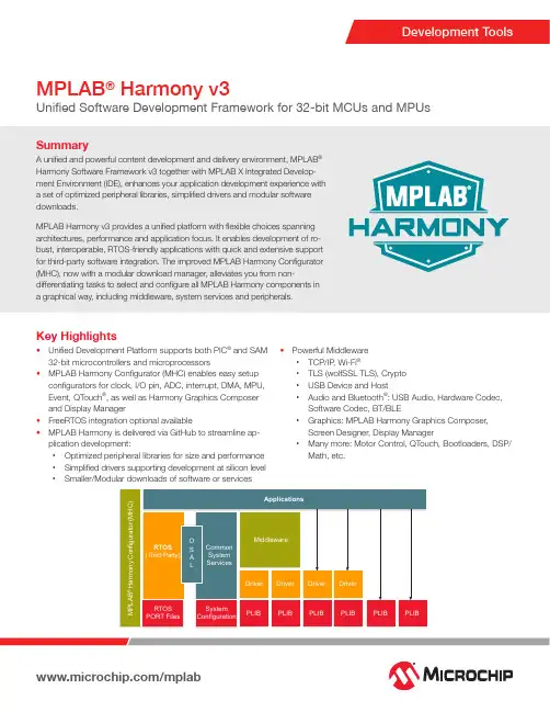
SummaryA unified and powerful content development and delivery environment, MPLAB ® Harmony Software Framework v3 together with MPLAB X Integrated Develop -ment Environment (IDE), enhances your application development experience with a set of optimized peripheral libraries, simplified drivers and modular software downloads.MPLAB Harmony v3 provides a unified platform with flexible choices spanning architectures, performance and application focus. It enables development of ro -bust, interoperable, RTOS-friendly applications with quick and extensive support for third-party software integration. The improved MPLAB Harmony Configurator (MHC), now with a modular download manager, alleviates you from non-differentiating tasks to select and configure all MPLAB Harmony components in a graphical way, including middleware, system services and peripherals.Development ToolsMPLAB ® Harmony v3Unified Software Development Framework for 32-bit MCUs and MPUsC: 100 M: 10 Y: 35 K: 15Key Highlights• Unified Development Platform supports both PIC® and SAM 32-bit microcontrollers and microprocessors•MPLAB Harmony Configurator (MHC) enables easy setup configurators for clock, I/O pin, ADC, interrupt, DMA, MPU, Event, QTouch®, as well as Harmony Graphics Composer and Display Manager• FreeRTOS integration optional available• MPLAB Harmony is delivered via GitHub to streamline ap -plication development:• Optimized peripheral libraries for size and performance • Simplified drivers supporting development at silicon level• Smaller/Modular downloads of software or services•Powerful Middleware• TCP/IP , Wi-Fi ®•TLS (wolfSSL TLS), Crypto • USB Device and Host• Audio and Bluetooth ®: USB Audio, Hardware Codec, Software Codec, BT/BLE• Graphics: MPLAB Harmony Graphics Composer, Screen Designer, Display Manager• Many more: Motor Control, QTouch, Bootloaders, DSP/Math, etc.The Microchip name and logo, the Microchip logo, MPLAB and PIC are registered trademarks of Microchip Technology Incorporated in the U.S.A. and other countries. Arm and Cortex are registered trademarks of Arm Limited (or its subsidiaries) in the EU and other countries. All other trademarks mentioned herein are property of their respective companies. © 2019, Microchip Technology Incorporated. All Rights Reserved. 7/19 DS00003024BTools and Demo ExamplesDevelopment KitsAvailable Resources• MPLAB Harmony v3 Landing Page: https:///mplab/mplab-harmony/mplab-harmony-v3• MPLAB Harmony v3 Device Support: https:///Microchip-MPLAB-Harmony/Micro -chip-MPLAB-Harmony.github.io/wiki/device_support• GitHub MPLAB Harmony v3 WiKi Page: https:///Microchip-MPLAB-Harmony/Microchip-MPLAB-Harmony.github.io/wiki• GitHub MPLAB Harmony v3 User Guide: https://microchip-mplab-harmony.github.io/Complementary Devices• Wireless Connectivity: Wi-Fi, Blue -tooth, BLE, LoRa, IEEE 802.15.4, Sub-G• Wired Connectivity and Interface: CAN Transceivers, Ethernt PHY • Industrial Networking: EtherCAT • CryptoAuthentication Device: ATECC608A, ATSHA204A• Clock and Timing: MEMs Oscillator • Analog: Op Amp, Motor Driver • Power Management: Linear and Switching RegulatorsServices and Third Party• Microchip Training: https:///training/• Third Party Solutions: https:///mplab/mplab-harmony/premium-products/third-party-solutions• ExpressLogic, FreeRTOS, Micrium, Segger and wolfSSL• Integrated Development Environment: IARATSAMC21N-XPRO/ATSAMD21-XPROThe SAMC21N/SAMD21 Xplained Pro Evaluation KitsATSAME54-XPRO/DM320113The SAM E54 Xplained Pro/The SAM E70 Explained Ultra Evaluation KitsDM320007-C/DM320010-CPIC32MZ EF (Connectivity)/PIC32MZ DA (Graphics) Starter KitsDM320104*The Curiosity PIC32MZEF Development Board, including on board Wi-Fi moduleATSAMV71-XULTThe SAM V71 Xplained Ultra evaluation kit is ideal for evaluating and prototyping with the SAM V71, SAM V70, SAM S70 and SAM E70 Arm ® Cortex ®-M7 based microcontrollers.ATSAMA5D2C-XULT*/SAMA5D27-SoM-EK1*The SAMA5D2 Xplained Ultra Evaluation Kit, including eMMC and DDR3/SoM and SiP Evaluation Kit*Harmony support coming soon。

© 2002 by Carnegie Mellon University
Version 1.5
page 5
Today’s talk
What is software architecture and why is it important? A benefit of architecture: Software product lines Evaluating software architectures
© 2002 by Carnegie Mellon University
Version 1.5
page 4
And yet...
It is still not well understood in some circles.
Some organizations have no “architect” position. Others have the position but it is informally defined. Some organizations are still proceeding to development without an architecture in place. The tools of the trade -- styles and patterns, views, evaluation -- are used sparingly if at all.
Version 1.5 page 1
1
The SEI: Who we are -1
The Software Engineering Institute (SEI) is • a federally funded research and development center • sponsored by the U. S. Department of Defense • hosted by Carnegie Mellon University in Pittsburgh • staffed by about 200 people

Lawrence RauchwergerDepartment of Computer Science phone:(979)845-8872 Texas A&M University fax:(979)458-0718 College Station,TX77843-3112email:rwerger@ USA url:/∼rwergerEducationPh.D.in Computer Science,University of Illinois at Urbana-Champaign,1995.Ph.D.Thesis:Run-Time Parallelization:A Framework for Parallel Computation.Thesis advisor:David Padua.M.S.in Electrical Engineering,Stanford University,1987.M.S.Research Area:Manufacturing Science and Technology for VLSI(Equipment Modeling).Engineer in Electronics and Telecommunications,Polytechnic Institute,Department of Electronic Engineering,1980,Bucharest,Romania.Diploma Project:Design and Implementation of an Alphanumeric and Graphic Display. Research InterestsCompilers for parallel and distributed computingParallel and distributed C++libraries.Adaptive runtime optimizations.Architectures for parallel computing.AwardsNSF Faculty Early Career Development(CAREER)Award,1998–2002.Elected Member,International Federation of Information Processing(IFIP),WG3.10,2003.TEES Fellow,College of Engineering,Texas A&M University2002-2003.TEES Fellow,College of Engineering,Texas A&M University2005-2006.TEES Select Young Faculty Award,College of Engineering,Texas A&M University2000-2001(awarded to two junior faculty each year by the College of Engineering).Best student paper award,co-authored with Silvius Rus,Int.Conference on Supercomputing,New York, NY,2002.Best student paper award,co-authored with Steve Saunders,Workshop on Performance Optimization for High-level Languages and Libraries,New York,NY,June2002.Intel Foundation Graduate Fellowship,1994.NASA(Langley)High Performance Computing Consortium(HPCC)Graduate Fellowship,1994. ExperienceProfessor,Department of Computer Science,Texas A&M University.(9/06–present)Co-Director,PARASOL Laboratory(3/98–present)Texas A&M University High Performance Computing Steering Committee.(1999–present)Visiting Professor,INRIA Futurs,Orsay,France.(9/04–11/04,7/06–8/06)IBM T.J.Watson Research Center,Yorktown Heights,NY.(10/03–8/04)Associate Professor,Department of Computer Science,Texas A&M University.(9/01–8/06)Assistant Professor,Department of Computer Science,Texas A&M University.(8/96–08/31/01) Visiting Scientist,AT&T Research Laboratories,Murray Hill,NJ.(6/96-8/96)Visiting Assistant Professor,Center for Supercomputing R&D,University of Illinois.(9/95-5/96) Research Assistant,Center for Supercomputing R&D,University of Illinois.(1/89-5/92,1/94-5/94) Teaching Assistant,Computer Science Department,University of Illinois.(1/93-12/93)Summer Intern,IBM T.J.Watson Research Center,Yorktown Heights,NY.(Summer1992)Research Assistant,Center for Integrated Systems,Stanford University.(1986–1988)R&D Engineer,Varian Associates Inc.,Thin Film Technology Division,R&D,Palo Alto,CA.(1984–1985)Design Engineer,Beckman Instruments Inc.,Scientific Instruments Division,Irvine,CA.(1983-1984) Design Engineer,The Felix Computer Company,R.&D.Department,Bucharest,Romania.(1980–1982)Research Grants“Adaptive Parallel Processing for Dynamic Applications”The National Science Foundation(CAREER Program)(CCR-9734471),PI:L.Rauchwerger,$237,000,(includes$10,000in REU Supplements, 1999,$27,000matching supplement,2000.)June1,1998–May31,2004.“CRS–AES:Collaborative Research:SoftCheck:Compiler and Run-Time Technology for Efficient Fault Detection and Correction in Low nm-Scale Multicore Chips,”The National Science Foundation PIs: Maria Garzaran(UIUC)and L.Rauchwerger$200,000,August2006–July2008.“STAPL:A High Productivity Parallel Programming Infrastructure,”Intel Corporation,PI:L.Rauchwerger,$30,000,November03,2005.“SmartApps:Middle-ware for Adaptive Applications on Reconfigurable Platforms,”The Department of Energy,Office of Science(Operating/Runtime Systems for Extreme Scale Scientific Computation Program),PI:L.Rauchwerger,co-PIs:M.Adams(Nuclear Engineering),N.Amato,B.Stroustrup, $1,500,000September1,2004–August31,2007.“ITR/NGS:STAPL:A Software Infrastructure for Computational Biology and Physics”(ACI-0326350), The National Science Foundation(Medium ITR Program),PI:L.Rauchwerger,co-PIs:N.Amato,B.Stroustrup,M.Adams(Nuclear Engineering),$416,000,November1,2003–October31,2007.“Efficient Massively Parallel Adaptive Algorithm for Time-Dependent Transport on Arbitrary Spatial Grids,”The Department of Energy,PI:M.Adams(Nuclear Engineering),co-PIs:N.Amato,P.Nel-son,L.Rauchwerger,$1,668,827,May1,2002–March31,2006.“Geometry Connectivity and Simulation of Cortical Networks”,Texas Higher Education Coordinating Board,PI:N.Amato co-PI:L.Rauchwerger$240,000January1,2002-August31,2004.“ITR/SY:Smart Apps:An Application Centric Approach to Scientific Computing”,The National Sci-ence Foundation(ACR-0113971),PI:L.Rauchwerger,co-PI:N.Amato,$463,809,September1, 2001–August31,2005.“ITR/AP:A Motion Planning Approach to Protein Folding Simulation”,The National Science Founda-tion(CCR-0113974),PI:N.Amato,co-PI:L.Rauchwerger,$318,000,September1,2001–August31,2005.“SmartApps:Smart Applications for Heterogeneous Computing,”(EIA-9975018),The National Science Foundation(Next Generation Software Program),PI:L.Rauchwerger,co-PI:N.Amato,J.Torrellas(Univ.Illinois at Urbana-Champaign),$610,000October1,1999–August31,2003.“PARASOL:An Adaptive Framework for Parallel Processing”(ACI-9872126),The National Science Foundation,PI:L.Rauchwerger,co-PI:N.Amato,$199,662,January1,1999–December31,2002.“Efficient Massively-Parallel Implementation of Modern Deterministic Transport Calculations”(B347886), Department of Energy(ASCI ASAP Level2and3Programs),PI:M.Adams(Nuclear Engineering),co-PIs:N.Amato,P.Nelson,L.Rauchwerger,$889,000,October21,1998–March31,2002.“Parallel Algorithms for Graph Cycle Detection,”Sandia National Laboratory,PI:L.Rauchwerger,$93,448,September1,1999–January15,2002.“Develop the How-to of a Qualified Compiler and Linker”,Aerospace Vehicle Space Institute(AVSI),PI:L.Rauchwerger,March01,2001–January31,2002.$45,500,Fellowship,Equipment,and Software Grants”CRI:A Cluster Testbed for Experimental Research in High Performance Computing”The National Science Foundation,PI:V.Taylor co-PI:N.Amato,L.Rauchwerger,$537,000,May15,2006–April30,2008.“Workshop NGS:Support for the Workshop on Languages and Compilers for Parallel Computing(LCPC),”The National Science Foundation,PI:Lawrence Rauchwerger,Co-PI:Nancy M.Amato,$15,000,September1,2003–August31,2004.“MRI:Development of Brain Tissue Scanner,”The National Science Foundation,PI:B.McCormick,co-PIs:N.Amato,J.Fallon(UCI),L.Rauchwerger,$105,000+$153,000funds from Texas A&M.September1,2000–July31,2001.“Education/Research Equipment Grant–HP V-class Shared Memory Multiprocessor Upgrade,”Hewlett-Packard,PI:Lawrence Rauchwerger and Nancy Amato,May2000,approximately$580,000.“Research Equipment Grant–16Processor V-class Shared Memory Multiprocessor Server,”Hewlett-Packard Co.,PI:L.Bhuyan,co-PIs:N.Amato,L.Rauchwerger,$1,200,000,1998.“Fellowships in Robotics,Training Science,Mobil Computing and High Performance Computing”(P200A80305), U.S.Department of Education(GAANN Fellowship Program),PI:R.V olz,co-PIs:N.Amato,L.Ev-erett,J.Welch,co-Investigators:L.Rauchwerger,J.Trinkle,N.Vaidya,J.Yen,Texas A&M Univer-sity,$601,224,August15,1998–August14,2001.Professional Service&ActivitiesNSF PanelistSeptember1998,October1998,June1999,November2000,May2002.Editorial Board MemberInt.Journal of Parallel Processing(IJPP),since2003.Guest Editor:Journal of Parallel Computing,Special Issue on Parallel Processing for Irregular Applications,2000.Int.Journal of Parallel Computing,2000,Special Issue on Selected Papers from ICS’99.Int.Journal of Parallel Computing,2002,Special Issue on Selected Papers from IWACT’2001.Program Chair16th Int.Conf.on Parallel Architectures and Compilation Techniques(PACT),2007.16th Workshop on Languages and Compilers for Parallel Computing(LCPC),2003.Program Committee Member:Int.Conf.for High Performance Computing and Communications(SC07),2007.Int.Parallel and Distributed Processing Symp.(IPDPS),2002,2006,2007.Int.W-shop on High-Level Parallel Programming Models and Supportive Environments(HIPS),2007.ACM Int.Conf.on Supercomputing(ICS),2000,2006,2007.Int.Conf.on High-Performance Embedded Architectures and Compilers(HiPEAC),Belgium,2007.Int.Conf.on High Performance Computing(HiPC),India,2000,2003,2007.Int.Conf.on Computer Design(ICCD),2006.Int.Conf.on High Performance Computing and Communications(HPCC),2006.ACM Int.Conf.on Computing Frontiers,Italy,2006.Int.IEEE W-shop on High Performance Computational Biology(HICOMB),2005;Int.Conf.on High Performance Computing and Communications(HPCC-05),Italy,2005;Workshop on Languages and Compilers for Parallel Computing(LCPC),2002,2004,2005;Workshop on Patterns in High Performance Computing,Champaign,IL,2005;ACM SIGPLAN Symp.Principles and Practice of Parallel Programming(PPoPP),2005;High Performance Computer Architecture Conf.(HPCA),2001,2002,2004;Int.Symp.on Parallel Architectures,Algorithms and Networks(I-SPAN),Philippines,2002;ACM Int.Conf.on Supercomputing(ICS’00),Santa Fe,NM,May2000;Int.Conf.on Parallel Processing(ICPP),1999,2000;Int.Conf.on Compiler Construction(CC),1999,2000;Int.Conf.on Parallel Architecture and Compilation Techniques(PACT),1999;First Workshop on Parallel Computing for Irregular Applications,Orlando,FL,January1999;Workshop and Publications Chair:High Performance Computer Architecture Conf.(HPCA-6),Toulouse,France,January2000.Exhibits Chair:ACM Int.Conf.on Supercomputing(ICS’02),New York,NY,June2002.Referee for Scientific Journals and Conferences.Member IEEE,ACM and IFIP WG3.10.Significant University and Departmental Service and ActivitiesTexas A&M University High Performance Computing Steering Committee,1999–present. Senator,Faculty Senate,Texas A&M University,2001–2005.Faculty Search Committee,2002–2003,2004–2005,2006–2007.Department Head Search Committee,2001–2002.Endowed Chair Search Committee,2001–2002.Computer Engineering Committee,2002-2003.Graduate Advisory Committee(GAC),2001–2002,2006–2007.Colloqium Committee.1998–1999,1999–2000,2001–2002(Chair).2002–2003(Chair).Advisory Committee2001-2002.Computer Services Advisory Committee,1997–1998.Graduate Admissions and Awards Committee,2000–2001,2004–2005,2006-2007.Library Committee.1998–1999,1999–2000(Chair).Total Quality Management(TQM).1997–1998.Courses TaughtGraduate:CPSC-605:Advanced Compiler Design(Fall96,97,98,99,00,01,02;Spring05,07)CPSC-614:Computer Architecture(Spring03)CPSC-654:Supercomputing(Spring99,01)CPSC-681:Graduate Seminar(Spring07)CPSC-689:Advanced Topics in Compiler Design(Spring00,02,03)CPSC-689:Special Topics:Runtime Systems for Parallel Computing(Spring06) Undergraduate:CPSC-434:Compiler Design(Spring97,98,99,00,01,02,05,06)CPSC-481:Undegraduate Seminar(Spring07)Student Research SupervisionGraduated PhD StudentsSilvius Rus,Ph.D.December2006,“Hybrid Analysis and its Application to Dynamic Compiler Opti-mization”Current position:Google,Mountain View,CA.Hao Yu,Ph.D.August2004,“Run-time Optimizations of Adaptive Irregular Applications.”Current position:Postdoc,IBM T.J.Watson Research Center,Yorktown Heights,NYYe Zhang,Ph.D.(UIUC)May1999,(co-advised with Prof.Josep Torrellas,University of Illinois),“Hardware for Speculative Run-time Parallelization in Distributed Shared-Memory Multiprocessors”, Current position:Software Engineer,Oracle Corporation,CA.Graduated Masters StudentsDevang Patel,M.S.August1998,“Compiler Integration of Speculative Run-Time Parallelization.”Cur-rent position:Software Engineer,Apple Computer,Sunnyvale,CA.Francisco Arzu,M.S.Summer2000,“STAPL:Standard Templates Adaptive Parallel Library.”Current position:Consultant and partner,,Austin,TXJulio Carvallo De Ochoa,M.S.,Summer2000,“Parallelization of Loops with Recurrence and Unknown Iteration Space”,Current position:Software Engineer,Wayne Industries,Austin,TX.William McLendon III,M.S.,Fall2001,“Parallel Detection and Elimination of Strongly Connected Components for Radiation and Transport Sweeps”,Current position:Software Engineer,Scalable Computing Systems Dept.,Sandia National Laboratory,Albuquerque,NM.Mothi Mohan Ram Thoppae,M.S.(EE),Fall2001,“Hardware and Software Co-techniques for Branch Prediction”,Current position:Component Design Engineer,Intel Corporation,Santa Clara,CA. Timmie Smith,M.C.S.,Summer2002,Current Position:Ph.D.Student,Texas A&M University,Dept.of Computer Science.Steven Saunders,M.S.,Spring2003,“A Parallel Communication Infrastructure for STAPL”,Current Position:Software Engineer,Raytheon,Dallas,TX.Current Graduate StudentsFrancis Dang,research area:Speculative Techniques,SmartApps.Alin Jula,research area:Parallel C++library,parallel dynamic memory management.Marinus Pennings,research area:Parallelizing Compilers,run-time optimization and compilation. Antoniu Pop,research area:Run-time systems,Operating Systems for SmartApps and STAPL. Nageswar Rao,research area:Run-time systems,Operating Systems for SmartApps and STAPL. Ioannis Papadopoulos,research area:Operating Systems for SmartApps and STAPL. Androniki Pazarloglu research area:Compilers.Timmie G.Smith,research area:Parallel C++Library,Parallel Memory Management.Gabriel Tanase,research area:Parallel C++Library,Nathan Thomas,research area:Parallel C++Library.Tao Huang,research area:Parallel C++Library.Undergraduate Research ProjectsWilliam Harris,Purdue University,Speculative Parallelization,Summer06.Aditya Awasthi,IIT,India,Summer06,STAPL.Saransh Mittal,IIT,India,Summer06,STAPL.Carson Brownle,Summer2005,CS REU Program.Visualization tool for graphs.Anna Tikhonova,Summer2005,CRA-W DMP Program,Parallel algorithms in STAPL. Armando Solar,Nuclear radiation transport simulation.01/01–07/03.Current Position:PhD student,UC BerkeleyReshma Ananthakrishnan,Test suite for STAPL,04/01–05/04.Current Position:Microsoft,Redmond,WAAndrew Cox,Software Branch Prediction,9/00-5/01.Current Position:Microsoft,Redmond,WA Steven Saunders,Java Parallel Library,1/00-12/00.Current Position:Raytheon,Dallas,TX Carrie Searcey,Java Parallel Library,5/00-8/00.Current Position:IBM,Raleigh,NCMichael Peter,Hardware for speculative run-time parallelization,1/99-7/99.Current Position:PhD student,TU Dresden,Germany.Francis Dang,Run-time parallelization(CPSC485project),6/98-6/99.Current Position:Supercomputing Center,Texas A&MWilliam McLendon,Performance Monitoring(CPSC485project),6/98-6/99.Current Position:Sandia National Labs,Albuquerque,NM.Timmie Smith,STAPL:Standard Parallel Adaptive C++Library,(CPSC485project)7/99-12/99.Current Position:PhD student.Texas A&M.Invited Presentations(Selected,last5years)“Automatic Parallelization with Hybrid Analysis”,IBM,T.J.Watson,Yorktown Heights,NY,April,2005.HP,Cupertino,CA,Feb.2006SIAM Conf.on Computational Science and Engineering,San Francisco,CA,February,2006.Compiler&Architecture Int.Seminar,IBM Haifa Research Labs,Haifa,Israel,December,2005.Fudan University,Shanghai,China,December,2005.“Efficient Massively Parallel Adaptive Algorithms for Time-Dependent Transport on Arbitrary Grids.”SIAM Conf.on Computational Science and Engineering,San Francisco,CA,February,2006.“SmartApps:Middleware for Adaptive Applications on Reconfigurable Platforms”,FAST-OS PI Meeting/Workshop,Rockville,MD,June,2005.“STAPL:A High Productivity Programming Infrastructure for Parallel&Distributed Computing”,Workshop on Patterns in High Performance Computing,Urbana,IL,May,2005.2005SIAM Conf.on Computational Science and Engineering,Orlando,FL,February,2005.“SmartApps:Adaptive Applications for High Productivity/High Performance”,UPC,Barcelona,Spain,December,2004Technical University,Delft,The Netherlands,November,2004Workshop on Scalable Approaches to High Performance and High Productivity Computing,Bertinoro Int.Center for Informatics(ScalPerf04),Italy,September2004.Universita di Pisa,Italy,November,2004.INRIA,Paris,France,2004.IBM,T.J.Watson,Yorktown Heights,NY,2004.“STAPL:A High Productivity Programming Infrastructure for Parallel and Distributed Computing”, Workshop on Domain Specific Languages for Numerical Optimization Argonne National Laboratory, August18-20,2004.IFIP WG3.10,London,UK,February,2004.“Memory Consistency Issues in STAPL”,DAGSTUHL Seminar:Hardware and Software Consistency Models:Programmability and Perfor-mance,Schloss Dagstuhl,Wadern,Germany,October2003.“Hybrid Analsyis”,DAGSTUHL Seminar:Emerging Technologies:Can Optimization Technology meet their Demands?, Schloss Dagstuhl,Wadern,Germany,February2003.“Compiler-Assisted Software and Hardware Support for Reduction Operations”,NSF Next Generation Software Workshop,Fort Lauderdale,FL,April2002.“STAPL:An Adaptive,Generic Parallel C++Library”,NSF Workshop on Software for the IBM Blue Gene Architecture,IBM T.J.Watson Research Center, April,2002.“Removing Architectural Bottlenecks to the Scalability of Speculative Parallelization”,IBM Research,Haifa,Israel,July2001.“SmartApps:An Application Centric Approach to High Performance Computing”,Workshop for Next Generation Software,San Francisco,CA,April,2001.Publications in Refereed Journals,Conferences and Workshops(Organized by topic;most papers available at /∼rwerger/) Compilers[1]A.Jula and L.Rauchwerger“Custom Memory Allocation for Free:Improving Data Locality withContainer-Centric Memory Allocation,”in Proc.of the19-th Workshop on Languages and Compilers for Parallel Computing(LCPC),New Orleans,Louisiana,Nov2006,to appear.[2]S.Rus,G.He and L.Rauchwerger,“Scalable Array SSA and Array Data Flow Analysis”,in Proc.ofthe18-th Workshop on Languages and Compilers for Parallel Computing(LCPC),Hawthorne,NY, 2005.Lecture Notes in Computer Science(LNCS),Springer-Verlag,to appear.[3]S.Rus,G.He,C.Alias and L.Rauchwerger,“Region Array SSA”,in Proc.of the15-th Int.Conf.on Parallel Architecture and Compilation Techniques(PACT),Seattle,WA,2006.[4]Hao Yu,Lawrence Rauchwerger,“An Adaptive Algorithm Selection Framework for Reduction Par-allelization”,IEEE Transactions on Parallel and Distributed Systems,17(19),2006,pp.1084–1096.[5]H.Yu,D.Zhang and L.Rauchwerger,“An Adaptive Algorithm Selection Framework”,in Proc.ofthe13th Int.Conf.on Parallel Architecture and Compilation Techniques(PACT),Antibes Juan-les-Pins,France,October,2004,pp.278–289.[6]S.Rus,D.Zhang and L.Rauchwerger,“The Value Evolution Graph and its Use in Memory ReferenceAnalysis”,in Proc.of the13th Int.Conf.on Parallel Architecture and Compilation Techniques (PACT),Antibes Juan-les-Pins,France,October,2004,pp.243–254.[7]S.Rus,D.Zhang and L.Rauchwerger,“Automatic Parallelization Using the Value Evolution Graph”,in Proc.of the17-th Workshop on Languages and Compilers for Parallel Computing(LCPC),West Lafayette,IN,2004.Also in Lecture Notes in Computer Science(LNCS),3602,Springer-Verlag, 2005,pp.379–393.[8]S.Rus,D.Zhang and L.Rauchwerger,“The Value Evolution Graph and its Use in Memory ReferenceAnalysis”,in Proc.of the11-th Workshop on Compilers for Parallel Computing(CPC),Seeon Monastery,Chiemsee,Germany,2004,pp.175–186.Invited Paper.[9]S.Rus,L.Rauchwerger and J.Hoeflinger,“Hybrid Analysis:Static&Dynamic Memory ReferenceAnalysis”,in Int.Journal of Parallel Programming,Special Issue,31(4),2003,pp.251–283.[10]H.Yu,F.Dang,and L.Rauchwerger,“Parallel Reductions:An Application of Adaptive AlgorithmSelection”,Proc.of the15-th Workshop on Languages and Compilers for Parallel Computing (LCPC),Washington,DC.,July,2002.Also in Lecture Notes in Computer Science(LNCS),Springer-Verlag,2481,2005,pp.188–202.[11]S.Rus,L.Rauchwerger and J.Hoeflinger,“Hybrid Analysis:Static&Dynamic Memory ReferenceAnalysis”,in Proc.of the ACM16-th Int.Conf.on Supercomputing(ICS02),New York,NY,June 2002,pp.274–284.Best Student Paper Award.[12]F.Dang,H.Yu and L.Rauchwerger,“The R-LRPD Test:Speculative Parallelization of PartiallyParallel Loops”,in Proc.of the Int.Parallel and Distributed Processing Symposium(IPDPS2002), Fort Lauderdale,FL,April2002,pp.20–30.[13]L.Rauchwerger,N.M.Amato and J.Torrellas,“SmartApps:An Application Centric Approach toHigh Performance Computing”,in Proc.of the13th Annual Workshop on Languages and Compilers for Parallel Computing(LCPC),Yorktown Heights,NY,August2000.Also in Lecture Notes in Computer Science,2017,Springer-Verlag,2000,pp.82–96.[14]F.Dang and L.Rauchwerger,“Speculative Parallelization of Partially Parallel Loops”,in Proc.of the5-th Workshop on Languages,Compilers,and Run-time Systems for Scalable Computers(LCR2000), Rochester,NY,May2000.Also in Lecture Notes in Computer Science,1915,2000,pp.285–299.[15]H.Yu and L.Rauchwerger,“Adaptive Reduction Parallelization”,in Proc.of the ACM14-th Int.Conf.on Supercomputing,(ICS’00),Santa Fe,NM,May2000,pp.66–77.[16]H.Yu and L.Rauchwerger,“Techniques for Reducing the Overhead of Run-time Parallelization”,in Proc.of the9th Int.Conf.on Compiler Construction(CC’00),Berlin,Germany,March2000, Lecture Notes in Computer Science,1781,Springer-Verlag,2000,pp.232–248.[17]L.Rauchwerger and D.Padua,“The LRPD Test:Speculative Run–Time Parallelization of Loopswith Privatization and Reduction Parallelization,”IEEE Transactions on Parallel and Distributed Systems,Special Issue on Compilers and Languages for Parallel and Distributed Computers,10(2), 1999,pp.160–180.[18]H.Yu and L.Rauchwerger,“Run-time Parallelization Optimization Techniques”,in Proc.of the12thAnnual Workshop on Languages and Compilers for Parallel Computing(LCPC),August1999,San Diego,CA.Also in Lecture Notes in Computer Science,1863,Springer-Verlag,2000,pp.481–484.[19]D.Patel and L.Rauchwerger,“Implementation Issues of Loop-level Speculative Run-time Paral-lelization”,Proc.of the8th Int.Conf.on Compiler Construction(CC’99),Amsterdam,The Nether-lands,March1999.Lecture Notes in Computer Science,1575,Springer-Verlag,1998,pp.183–197.[20]Lawrence Rauchwerger,“Run-Time Parallelization:It’s Time Has Come”,Journal of Parallel Com-puting,Special Issue on Languages&Compilers for Parallel Computers,24(3–4),1998,pp.527–556.[21]D.Patel and L.Rauchwerger,“Principles of Speculative Run-time Parallelization”,Proc.of the11th Annual Workshop on Languages and Compilers for Parallel Computing(LCPC),August1998, Chapel Hill,NC.Also in Lecture Notes in Computer Science,1656,Springer-Verlag,1998,pp.323–337.[22]W.Blume,R.Doallo,R.Eigenmann,J.Grout,J.Hoeflinger,wrence,J.Lee,D.Padua,Y.Paek,W.Pottenger,L.Rauchwerger,and P.Tu,“Advanced Program Restructuring for High-Performance Computers with Polaris,”IEEE Computer,29(12),1996,pp.78–82.[23]W.Blume,R.Eigenmann,K.Faigin,J.Grout,J.Lee,wrence,J.Hoeflinger,D.Padua,Y.Paek,P.Petersen,B.Pottenger,L.Rauchwerger,P.Tu,and S.Weatherford,“Restructuring Programs for High-Speed Computers with Polaris”,Proc.of the1996ICPP Workshop on Challenges for Parallel Processing,August1996,pp.149–162.[24]L.Rauchwerger,N.M.Amato and D.Padua,“A Scalable Method for Run-Time Loop Paralleliza-tion,”Int.Journal of Parallel Programming,23(6),1995,pp.537–576.(CSRD Tech.Rept.1400.)[25]L.Rauchwerger,N.M.Amato and D.Padua,“Run-Time Methods for Parallelizing Partially ParallelLoops,”Proc.of the9th ACM Int.Conf.on Supercomputing(ICS’95),July1995,Barcelona,Spain, pp.137–146.[26]L.Rauchwerger and D.Padua,“The LRPD Test:Speculative Run–Time Parallelization of Loopswith Privatization and Reduction Parallelization,”Proc.of the ACM SIGPLAN1995Conf.on Pro-gramming Language Design and Implementation(PLDI95),June1995,La Jolla,CA.,pp.218–232.[27]L.Rauchwerger and D.Padua,“Parallelizing While Loops for Multiprocessor Systems,”Proc.ofthe9th Int.Parallel Processing Symposium,April1995,Santa Barbara,CA,pp.347–356.[28]L.Rauchwerger and D.Padua,“The Privatizing DOALL Test:A Run-Time Technique for DOALLLoop Identification and Array Privatization,”Proc.8th ACM Int.Conf.on Supercomputing,July 1994,Manchester,England,pp.33–43.[29]W.Blume,R.Eigenmann,J.Hoeflinger,D.Padua,P.Petersen,L.Rauchwerger and P.Tu,“AutomaticDetection of Parallelism:A Grand Challenge for High-Performance Computing,”IEEE Parallel and Distributed Technology,Systems and Applications-Special Issue on High Performance Fortran,Fall 1994,2(3),pp.37–47.[30]W.Blume,R.Eigenmann,K.Faigin,J.Grout,J.Hoeflinger,D.Padua,P.Petersen,B.Pottenger,L.Rauchwerger,P.Tu,and S.Weatherford,“Polaris:Improving the Effectiveness of Parallelizing Compilers,”Proc.7th Ann.Workshop on Languages and Compilers for Parallel Computing(LCPC), August1994,Ithaca,New York;Also in Lecture Notes in Computer Science,892,Springer-Verlag, 1994,pp.141–154.[31]L.Rauchwerger and D.Padua,“Run-Time Methods for Parallelizing DO Loops,”Proc.of the2ndInt.Workshop on Massive Parallelism:Hardware,Software and Applications,October1994,Capri, Italy,pp.1–15.Parallel Libraries&Applications[32]Lawrence Rauchwerger and Nancy Amato,“SmartApps:Middle-ware for Adaptive Applications onReconfigurable Platforms”,ACM SIGOPS Operating Systems Reviews,Special Issue on Operating and Runtime Systems for High-End Computing Systems,40(2):73–82,2006.[33]N.Thomas,S.Saunders,T.Smith,G.Tanase,L.Rauchwerger,“ARMI:A High Level Communica-tion Library for STAPL,”Parallel Processing Letters,June,2006,16(2):261-280.[34]W.McLendon III,B.Hendrickson,S.Plimpton,L.Rauchwerger,“Finding strongly connected com-ponents in distributed graphs”,Journal of Parallel and Distributed Computing(JPDC),March,2005.65(8):901-910,2005.[35]N.Thomas,G.Tanase,achyshyn,J.Perdue,N.M.Amato,L.Rauchwerger,“A Framework forAdaptive Algorithm Selection in STAPL”,in Proc.of ACM SIGPLAN Symposium on Principles and Practice of Parallel Programming(PPOPP),Chicago,IL,June,2005,pp.277–288.[36]Shawna Thomas,Gabriel Tanase,Lucia K.Dale,Jose E.Moreira,Lawrence Rauchwerger,NancyM.Amato,“Parallel Protein Folding with STAPL,”Concurrency and Computation:Practice and Experience,17(14),2005,pp.1643–1656.[37]Steven J.Plimpton,Bruce Hendrickson,Shawn Burns,William McLendon III and Lawrence Rauch-werger,“Parallel Algorithms for S n Transport on Unstructured Grids”,Journal of Nuclear Science and Engineering,150(7),2005,pp.1-17.[38]S.Saunders and L.Rauchwerger,“ARMI:An Adaptive,Platform Independent Communication Li-brary”,in Proc.of ACM SIGPLAN Symposium on Principles and Practice of Parallel Programming (PPOPP),San Diego,CA,June,2003,pp.230–241.[39]S.Saunders and L.Rauchwerger,“A Parallel Communication Infrastructure for STAPL”,in Proc.ofthe Workshop on Performance Optimization for High-level Languages and Libraries(POHLL-02), New York,NY,June2002Best Student Paper Award.[40]P.An,A.Jula,S.Rus,S.Saunders,T.Smith,G.Tanase,N.Thomas,N.M.Amato and L.Rauch-werger,“STAPL:An Adaptive,Generic Parallel C++Library”,in Proc.of the14-th Workshop on Languages and Compilers for Parallel Computing(LCPC),Cumberland Falls,KY,August2001.Also in Lecture Notes in Computer Science(LNCS),2624Springer-Verlag,2003,pp.193–208. [41]W.McLendon III,Bruce Hendrickson,S.Plimpton,L.Rauchwerger,“Finding Strongly ConnectedComponents in Parallel in Particle Transport Sweeps”,in Proc.of13-th Symposium on Parallel Algorithms and Architectures,(SPAA)Crete,Greece,July2001,pp.141–154.[42]L.Rauchwerger,F.Arzu and K.Ouchi,“Standard Templates Adaptive Parallel Library”,Proc.of the4th Int.Workshop on Languages,Compilers and Run-Time Systems for Scalable Computers(LCR), May1998,Pittsburgh,PA;Also in Lecture Notes in Computer Science,1511,Springer-Verlag,1998, pp.402–410.Computer Architecture[43]M.Garzaran,M.Prvulovic,J.Llaberia,V.Vinals,L.Rauchwerger,and J.Torrellas,“Tradeoffsin Buffering Speculative Memory State for Thread-Level Speculation in Multiprocessors”in ACM Transactions on Architecture and Code Optimization(TACO),2(3):247-279,September2005. [44]R.Iyer,J.Perdue,L.Rauchwerger,N.M.Amato,L.Bhuyan,“An Experimental Evaluation of the HPV-Class and SGI Origin2000Multiprocessors using Microbenchmarks and Scientific Applications,”Int.J.of Parallel Programming,33(4),2005,pp.307–350.[45]M.Garzar´a n,M.Prvulovic,V.Vials,J.Llabera,L.Rauchwerger,and J.Torrellas,“Software Loggingunder Speculative Parallelization”,in Proc.of Workshop on High Performance Memory Systems, Goteborg,Sweden,June2001,extended version in Chapter of“High Performance Memory Systems”,Editors:Haldun Hadimioglu, David Kaeli,Jeffrey Kuskin,Ashwini Nanda,and Josep Torrellas,pp.181-193,Springer-Verlag, November2003,ISBN0-387-00310-X.[46]M.Garzar´a n,M.Prvulovic,J.Llaberia,V.Vinals,L.Rauchwerger,and J.Torrellas,“Tradeoffs inBuffering Memory State for Thread-Level Speculation in Multiprocessors”,in Proc.of Conf.on High Performance Computer Architecture2003,(HPCA),Anaheim,CA.,Feb.8-12,2003. [47]M.Garzar´a n,M.Prvulovic,V.Vials,J.Llabera,L.Rauchwerger,and J.Torrellas,“Using SoftwareLogging to Support Multi-Version Buffering in Thread-Level Speculation”,in Proc.of the Int.Conf.on Parallel Architectures and Compilation Techniques(PACT),September2003,pp.170-181. [48]M.Garzar´a n,A.Jula,M.Prvulovic,H.Yu,L.Rauchwerger,and J.Torrellas,“Architectural Supportfor Parallel Reductions in Scalable Shared-Memory Multiprocessors”,in Proc.of the6-th Int.Conf.on Parallel Computing Technologies(PACT),September,2001,pp.243–254.[49]M.Prvulovic,M.Garzar´a n,L.Rauchwerger,and J.Torrellas,“Removing Architectural Bottlenecksto the Scalability of Speculative Parallelization”,in Proc.of the28-th Int.Symp.on Computer Architecture(ISCA),Goteborg,Sweden,June2001,pp.204–215.[50]Y.Zhang,L.Rauchwerger and J.Torrellas,Hardware for Speculative Parallelization in High-EndMultiprocessors The Third PetaFlop Workshop(TPF-3),Annapolis,February1999.。

[转载]k-折交叉验证（K-fold cross-validation）原⽂地址：k-折交叉验证（K-fold cross-validation）作者：清风⼩荷塘k-折交叉验证（K-fold cross-validation）是指将样本集分为k份，其中k-1份作为训练数据集，⽽另外的1份作为验证数据集。

⽤验证集来验证所得分类器或者回归的错误码率。

⼀般需要循环k次，直到所有k份数据全部被选择⼀遍为⽌。

Cross validation is a model evaluation method that is better than residuals. The problem with residual evaluations is that they do not give an indication of how well the learner will do when it is asked to make new predictions for data it has not already seen. One way to overcome this problem is to not use the entire data set when training a learner. Some of the data is removed before training begins. Then when training is done, the data that was removed can be used to test the performance of the learned model on ``new'' data. This is the basic idea for a whole class of model evaluation methods called cross validation.The holdout method is the simplest kind of cross validation. The data set is separated into two sets, called the training set and the testing set. The function approximator fits a function using the training set only. Then the function approximator is asked to predict the output values for the data in the testing set (it has never seen these output values before). The errors it makes are accumulated as before to give the mean absolute test set error, which is used to evaluate the model. The advantage of this method is that it is usually preferable to the residual method and takes no longer to compute. However, its evaluation can have a high variance. The evaluation may depend heavily on which data points end up in the training set and which end up in the test set, and thus the evaluation may be significantly different depending on how the division is made.K-fold cross validation is one way to improve over the holdout method. The data set is divided into k subsets, and the holdout method is repeated k times. Each time, one of the k subsets is used as the test set and the other k-1 subsets are put together to form a training set. Then the average error across all k trials is computed. The advantage of this method is that it matters less how the data gets divided. Every data point gets to be in a test set exactly once, and gets to be in a training set k-1 times. The variance of the resulting estimate is reduced as k is increased. The disadvantage of this method is that the training algorithm has to be rerun from scratch k times, which means it takes k times as much computation to make an evaluation. A variant of this method is to randomly divide the data into a test and training set k different times. The advantage of doing this is that you can independently choose how large each test set is and how many trials you average over.Leave-one-out cross validation is K-fold cross validation taken to its logical extreme, with K equal to N, the number of da ta points in the set. That means that N separate times, the function approximator is trained on all the data except for one point and a prediction is made for that point. As before the average error is computed and used to evaluate the model. The evaluation given by leave-one-out cross validation error (LOO-XVE) is good, but at first pass it seems very expensive to compute. Fortunately, locally weighted learners can make LOO predictions just as easily as they make regular predictions. That means computing the LOO-XVE takes no more time than computing the residual error and it is a much better way to evaluate models. We will see shortly that Vizier relies heavily on LOO-XVE to choose its metacodes.Figure 26: Cross validation checks how well a model generalizes to new dataFig. 26 shows an example of cross validation performing better than residual error. The data set in the top two graphs is a simple underlying function with significant noise. Cross validation tells us that broad smoothing is best. The data set in the bottom two graphs is a complex underlying function with no noise. Cross validation tells us that very little smoothing is best for this data set.Now we return to the question of choosing a good metacode for data set a1.mbl:File -> Open -> a1.mblEdit -> Metacode -> A90:9Model -> LOOPredictEdit -> Metacode -> L90:9Model -> LOOPredictEdit -> Metacode -> L10:9Model -> LOOPredictLOOPredict goes through the entire data set and makes LOO predictions for each point. At the bottom of the page itshows the summary statistics including Mean LOO error, RMS LOO error, and information about the data point with the largest error. The mean absolute LOO-XVEs for the three metacodes given above (the same three used to generate the graphs in fig. 25), are 2.98, 1.23, and 1.80. Those values show that global linear regression is the best metacode of those three, which agrees with our intuitive feeling from looking at the plots in fig. 25. If you repeat the above operation on data set b1.mbl you'll get the values 4.83, 4.45, and 0.39, which also agrees with our observations.What are cross-validation and bootstrapping?--------------------------------------------------------------------------------Cross-validation and bootstrapping are both methods for estimatinggeneralization error based on "resampling" (Weiss and Kulikowski 1991; Efronand Tibshirani 1993; Hjorth 1994; Plutowski, Sakata, and White 1994; Shaoand Tu 1995). The resulting estimates of generalization error are often usedfor choosing among various models, such as different network architectures.Cross-validation++++++++++++++++In k-fold cross-validation, you divide the data into k subsets of(approximately) equal size. You train the net k times, each time leavingout one of the subsets from training, but using only the omitted subset tocompute whatever error criterion interests you. If k equals the samplesize, this is called "leave-one-out" cross-validation. "Leave-v-out" is amore elaborate and expensive version of cross-validation that involvesleaving out all possible subsets of v cases.Note that cross-validation is quite different from the "split-sample" or"hold-out" method that is commonly used for early stopping in NNs. In thesplit-sample method, only a single subset (the validation set) is used toestimate the generalization error, instead of k different subsets; i.e.,there is no "crossing". While various people have suggested thatcross-validation be applied to early stopping, the proper way of doing so isnot obvious.The distinction between cross-validation and split-sample validation isextremely important because cross-validation is markedly superior for smalldata sets; this fact is demonstrated dramatically by Goutte (1997) in areply to Zhu and Rohwer (1996). For an insightful discussion of thelimitations of cross-validatory choice among several learning methods, seeStone (1977).Jackknifing+++++++++++Leave-one-out cross-validation is also easily confused with jackknifing.Both involve omitting each training case in turn and retraining the networkon the remaining subset. But cross-validation is used to estimategeneralization error, while the jackknife is used to estimate the bias of astatistic. In the jackknife, you compute some statistic of interest in eachsubset of the data. The average of these subset statistics is compared withthe corresponding statistic computed from the entire sample in order toestimate the bias of the latter. You can also get a jackknife estimate ofthe standard error of a statistic. Jackknifing can be used to estimate thebias of the training error and hence to estimate the generalization error,but this process is more complicated than leave-one-out cross-validation(Efron, 1982; Ripley, 1996, p. 73).Choice of cross-validation method+++++++++++++++++++++++++++++++++Cross-validation can be used simply to estimate the generalization error of a given model, or it can be used for model selection by choosing one of several models that has the smallest estimated generalization error. For example, you might use cross-validation to choose the number of hidden units, or you could use cross-alidation to choose a subset of the inputs (subset selection). A subset that contains all relevant inputs will be called a "good" subsets, while the subset that contains all relevant inputs but no others will be called the "best" subset. Note that subsets are "good" and "best" in an asymptotic sense (as the number of training cases goes to infinity). With a small training set, it is possible that a subset that is smaller than the "best" subset may provide better generalization error.Leave-one-out cross-validation often works well for estimating generalization error for continuous error functions such as the mean squared error, but it may perform poorly for discontinuous error functions such as the number of misclassified cases. In the latter case, k-fold cross-validation is preferred. But if k gets too small, the error estimate is pessimistically biased because of the difference in training-set size between the full-sample analysis and the cross-validation analyses. (For model-selection purposes, this bias can actually help; see the discussion below of Shao, 1993.) A value of 10 for k is popular for estimating generalization error.Leave-one-out cross-validation can also run into trouble with variousmodel-selection methods. Again, one problem is lack of continuity--a smallchange in the data can cause a large change in the model selected (Breiman,1996). For choosing subsets of inputs in linear regression, Breiman andSpector (1992) found 10-fold and 5-fold cross-validation to work better thanleave-one-out. Kohavi (1995) also obtained good results for 10-foldcross-validation with empirical decision trees (C4.5). Values of k as smallas 5 or even 2 may work even better if you analyze several different randomk-way splits of the data to reduce the variability of the cross-validationestimate.Leave-one-out cross-validation also has more subtle deficiencies for modelselection. Shao (1995) showed that in linear models, leave-one-outcross-validation is asymptotically equivalent to AIC (and Mallows' C_p), butleave-v-out cross-validation is asymptotically equivalent to Schwarz's Bayesian criterion (called SBC or BIC) when v =n[1-1/(log(n)-1)], where n is the number of training cases. SBCprovides consistent subset-selection, while AIC does not. That is, SBC will choose the "best" subset with probability approaching one as the size of the training set goes to infinity. AIC has an asymptotic probability of one of choosing a "good" subset, but less than one of choosing the "best" subset (Stone, 1979). Many simulation studies have also found that AIC overfits badly in small samples, and that SBC works well (e.g., Hurvich and Tsai, 1989; Shao and Tu, 1995). Hence, these results suggest that leave-one-out cross-validation should overfit in small samples, but leave-v-outcross-validation with appropriate v should do better. However, when true models have an infinite number of parameters, SBC is not efficient, and other criteria that are asymptotically efficient but not consistent formodel selection may produce better generalization (Hurvich and Tsai, 1989). Shao (1993) obtained the surprising result that for selecting subsets of inputs in a linear regression, the probability of selecting the "best" doesnot converge to 1 (as the sample size n goes to infinity) for leave-v-out cross-validation unless the proportion v/n approaches 1. At first glance, Shao's result seems inconsistent with the analysis by Kearns (1997) ofsplit-sample validation, which shows that the best generalization is obtained with v/n strictly between 0 and 1, with little sensitivity to the precise value of v/n for large data sets. But the apparent conflict is dueto the fundamentally different properties of cross-validation andsplit-sample validation.To obtain an intuitive understanding of Shao (1993), let's review some background material on generalization error. Generalization error can be broken down into three additive parts, noise variance + estimation variance + squared estimation bias. Noise variance is the same for all subsets of inputs. Bias is nonzero for subsets that are not "good", but it's zero forall "good" subsets, since we are assuming that the function to be learned is linear. Hence the generalization error of "good" subsets will differ only in the estimation variance. The estimation variance is (2p/t)s^2 where pis the number of inputs in the subset, t is the training set size, and s^2is the noise variance. The "best" subset is better than other "good" subsetsonly because the "best" subset has (by definition) the smallest value of p. But the t in the denominator means that differences in generalization error among the "good" subsets will all go to zero as t goes to infinity.Therefore it is difficult to guess which subset is "best" based on the generalization error even when t is very large. It is well known that unbiased estimates of the generalization error, such as those based on AIC, FPE, and C_p, do not produce consistent estimates of the "best" subset (e.g., see Stone, 1979).In leave-v-out cross-validation, t=n-v. The differences of thecross-validation estimates of generalization error among the "good" subsets contain a factor 1/t, not 1/n. Therefore by making t small enough (and thereby making each regression based on t cases bad enough), we can make the differences of the cross-validation estimates large enough to detect. It turns out that to make t small enough to guess the "best" subset consistently, we have to have t/n go to 0 as n goes to infinity.The crucial distinction between cross-validation and split-sample validation is that with cross-validation, after guessing the "best" subset, we trainthe linear regression model for that subset using all n cases, but withsplit-sample validation, only t cases are ever used for training. If ourmain purpose were really to choose the "best" subset, I suspect we would still have to have t/n go to 0 even for split-sample validation. Butchoosing the "best" subset is not the same thing as getting the best generalization. If we are more interested in getting good generalizationthan in choosing the "best" subset, we do not want to make our regression estimate based on only t cases as bad as we do in cross-validation, because in split-sample validation that bad regression estimate is what we're stuck with. So there is no conflict between Shao and Kearns, but there is a conflict between the two goals of choosing the "best" subset and getting the best generalization in split-sample validation.Bootstrapping+++++++++++++Bootstrapping seems to work better than cross-validation in many cases (Efron, 1983). In the simplest form of bootstrapping, instead of repeatedly analyzing subsets of the data, you repeatedly analyze subsamples of the data. Each subsample is a random sample with replacement from the fullsample. Depending on what you want to do, anywhere from 50 to 2000 subsamples might be used. There are many more sophisticated bootstrap methods that can be used not only for estimating generalization error butalso for estimating confidence bounds for network outputs (Efron and Tibshirani 1993). For estimating generalization error in classification problems, the .632+ bootstrap (an improvement on the popular .632 bootstrap) is one of the currently favored methods that has the advantage of performing well even when there is severe overfitting. Use of bootstrapping for NNs is described in Baxt and White (1995), Tibshirani (1996), and Masters (1995). However, the results obtained so far are not very thorough, and it is known that bootstrapping does not work well for some other methodologies such as empirical decision trees (Breiman, Friedman, Olshen, and Stone, 1984; Kohavi, 1995), for which it can be excessively optimistic.For further information+++++++++++++++++++++++Cross-validation and bootstrapping become considerably more complicated for time series data; see Hjorth (1994) and Snijders (1988).More information on jackknife and bootstrap confidence intervals is available at ftp:///pub/neural/jackboot.sas (this is a plain-text file).References:Baxt, W.G. and White, H. (1995) "Bootstrapping confidence intervals forclinical input variable effects in a network trained to identify thepresence of acute myocardial infarction", Neural Computation, 7, 624-638. Breiman, L., and Spector, P. (1992), "Submodel selection and evaluationin regression: The X-random case," International Statistical Review, 60,291-319.Dijkstra, T.K., ed. (1988), On Model Uncertainty and Its StatisticalImplications, Proceedings of a workshop held in Groningen, TheNetherlands, September 25-26, 1986, Berlin: Springer-Verlag.Efron, B. (1982) The Jackknife, the Bootstrap and Other ResamplingPlans, Philadelphia: SIAM.Efron, B. (1983), "Estimating the error rate of a prediction rule:Improvement on cross-validation," J. of the American StatisticalAssociation, 78, 316-331.Efron, B. and Tibshirani, R.J. (1993), An Introduction to the Bootstrap,London: Chapman & Hall.Efron, B. and Tibshirani, R.J. (1997), "Improvements on cross-validation: The .632+ bootstrap method," J. of the American Statistical Association, 92, 548-560.Goutte, C. (1997), "Note on free lunches and cross-validation," NeuralComputation, 9, 1211-1215,ftp://eivind.imm.dtu.dk/dist/1997/goutte.nflcv.ps.gz.Hjorth, J.S.U. (1994), Computer Intensive Statistical Methods Validation, Model Selection, and Bootstrap, London: Chapman & Hall.Hurvich, C.M., and Tsai, C.-L. (1989), "Regression and time series model selection in small samples," Biometrika, 76, 297-307.Kearns, M. (1997), "A bound on the error of cross validation using theapproximation and estimation rates, with consequences for thetraining-test split," Neural Computation, 9, 1143-1161.Kohavi, R. (1995), "A study of cross-validation and bootstrap foraccuracy estimation and model selection," International Joint Conference on Artificial Intelligence (IJCAI), pp. ?,/users/ronnyk/Masters, T. (1995) Advanced Algorithms for Neural Networks: A C++Sourcebook, NY: John Wiley and Sons, ISBN 0-471-10588-0Plutowski, M., Sakata, S., and White, H. (1994), "Cross-validationestimates IMSE," in Cowan, J.D., Tesauro, G., and Alspector, J. (eds.)Advances in Neural Information Processing Systems 6, San Mateo, CA: Morgan Kaufman, pp. 391-398.Ripley, B.D. (1996) Pattern Recognition and Neural Networks, Cambridge: Cambridge University Press.Shao, J. (1993), "Linear model selection by cross-validation," J. of theAmerican Statistical Association, 88, 486-494.Shao, J. (1995), "An asymptotic theory for linear model selection,"Statistica Sinica ?.Shao, J. and Tu, D. (1995), The Jackknife and Bootstrap, New York:Springer-Verlag.Snijders, T.A.B. (1988), "On cross-validation for predictor evaluation intime series," in Dijkstra (1988), pp. 56-69.Stone, M. (1977), "Asymptotics for and against cross-validation,"Biometrika, 64, 29-35.Stone, M. (1979), "Comments on model selection criteria of Akaike and Schwarz," J. of the Royal Statistical Society, Series B, 41, 276-278.Tibshirani, R. (1996), "A comparison of some error estimates for neural network models," Neural Computation, 8, 152-163.Weiss, S.M. and Kulikowski, C.A. (1991), Computer Systems That Learn, Morgan Kaufmann.Zhu, H., and Rohwer, R. (1996), "No free lunch for cross-validation,"Neural Computation, 8, 1421-1426.。

EVB_RT7276GQWRT7276GQWEvaluation BoardPurposeThe RT7276 is a high-performance 700kHz 3A step down regulator with an internal power switch and synchronous rectifier. This document explains the function and use of the RT7276 evaluation board (EVB) and provides information to enable operation and modification of the evaluation board and circuit to suit individual requirements.Table of ContentsPurpose (1)Introduction (2)General Product Information (2)Key Performance Summary Table (3)Bench Test Setup Conditions (4)Headers Description and Placement (4)Test Points (5)Power-up & Measurement Procedure (5)Output Voltage Setting (5)Schematic, Bill of Materials and Board Layout (6)EVB Schematic Diagram (6)Bill of Materials (7)EVB Layout (8)Other Technical Information (11)Evaluation Board IntroductionGeneral Product InformationGeneral DescriptionThe RT7276 is a high-performance 700kHz 3A step down regulator with an internal power switch and synchronous rectifier. It features quick transient response using its Advanced Constant On-Time (ACOT TM) control architecture that provides stable operation with small ceramic output capacitors and without complicated external compensation, among other benefits. The input voltage range is from 4.5V to 18V and the output is adjustable from 0.765V to 8V. The proprietary ACOT TM control improves upon other fast response constant on-time architectures, achieving nearly constant switching frequency over line, load, and output voltage ranges. Since there is no internal clock, response to transients is nearly instantaneous and inductor current can ramp quickly to maintain output regulation without large bulk output capacitance. The RT7276 is stable with and optimized for ceramic output capacitors.With its internal 90mΩ switch and 60mΩ synchronous rectifier, the RT7276 displays excellent efficiency and good behavior across a range of applications, especially for low output voltages and low duty cycles. Cycle-by cycle current limit, input under-voltage lock-out, externally-adjustable soft-start, output under- and overvoltage protection, and thermal shutdown provide safe and smooth operation in all operating conditions.The RT7276 evaluation board uses the RT7276GQW IC in a WDFN-10L3x3 package with an exposed thermal pad. The IC is also available in a PTSSOP-14 package with an exposed thermal pad.Features●Fast Transient Response●Steady 700kHz Switching Frequency at PWM●3A Output Current●Advanced Constant On-Time (ACOT TM) Control●Optimized for Ceramic Output Capacitors● 4.5V to 18V Input Voltage Range●Internal 90mΩ Switch and 60mΩ Synchronous Rectifier●0.765V to 8V Adjustable Output Voltage●Externally-adjustable, Pre-biased Compatible Soft-Start●Cycle-by-Cycle Current Limit●Output Over- and Under-voltage Shut-downEvaluation BoardKey Performance Summary TableKey features Evaluation board number: PCB002_V1 Default Input voltage 12VMax Output Current 3ADefault Output Voltage 1.05VDefault Marking & Package Type RT7276GQW (WDFN-10L 3x3)Operation Frequency Steady 700kHz at PWMOther Key Features Advanced constant On-time(ACOT TM) controlPower GoodAdjustable Soft-start (external capacitor)PSM/ PWM Auto SwitchedProtection Over current protection:Cycle-by-Cycle Current LimitHiccup Mode Output Over- and Under-voltage Shut-downEvaluation Board Bench Test Setup ConditionsHeaders Description and PlacementPlease carefully inspect the EVB IC and external components, comparing them to thefollowing Bill of Materials, to ensure that all components are installed and undamaged. If anycomponents are missing or damaged during transportation, please contact the distributor or***********************************.Evaluation BoardTest PointsThe EVB is provided with the test points and pin names listed in the table below.Test point/Pin nameSignal Comment (expected waveforms or voltage levels on test points) VIN Input voltage Input voltage range = 4.5V to 18VVOUT Outputvoltage Default output voltage = 1.05VOutput voltage range = 0.765V to 8V(see ‘’ Output Voltage Setting’’ section for changing output voltage level) GND Ground Ground reference for the input voltage, output voltage and analog ground SW Switching node test point SW waveformEN Enable test point Enable signal. Drive EN or install a shorting block on Jumper JP1 toenable operation (shorting 2-3) or disable operation (shorting 1-2).JP1 Chip enable control Install jumper or drive EN directly to enable or disable operationBOOT Boot strap supply test point Floating supply voltage for the high-side N-MOSFET switchSS Soft-start control test point Soft start waveformPVCC Linear regulator output testpointInternal linear regulator output= 5.1VPG Power good output testpoint Connected to PVCC through R29, PG voltage is 5.1V when soft-start is complete and the output voltage is in regulationPower-up & Measurement Procedure1. Connect a jumper at JP1 terminals 1 and 2, connecting EN to GND, to disable operation.2. Apply a 12V nominal input power supply (4.5V < V IN < 18V) to the VIN and GND terminals.3. Set the jumper at JP1 to connect terminals 2 and 3, connecting EN to VIN through resistor R30, to enableoperation.4. Verify the output voltage (approximately 1.05V) between VOUT and GND.5. Connect an external load up to 3A to the VOUT and GND terminals and verify the output voltage and current.Output Voltage SettingSet the output voltage with the resistive divider (R23, R28) between VOUT and GND with the midpoint at FB. The output is set by the following formula:OUT R23V = 0.765 x (1 + )R28The installed V OUT capacitors (C11, C12) are 22μF, 16V X5R ceramic types. Do not exceed their operating voltage range and consider their voltage coefficient (capacitance vs. bias voltage) and ensure that the capacitance is sufficient to maintain stability and provide sufficient transient response for your application. Installing a small 5pF to 22pF capacitor at C30 (in parallel with R23) may be desirable to improve transient response for higher output voltages. See the RT7276 IC datasheet for more information.Evaluation BoardSchematic, Bill of Materials and Board LayoutEVB Schematic DiagramR2910k TP1PGTP2PVCCTP3ENTP4SSVIN TP5BOOTL2NFGNDU5WDFN-10L 3x3EN1FB2PVCC3SS4VIN10VIN 9BOOT 8SW7PG 5SW 6G N D11TP6JP1EN 123R30100kR2822kR238.2kC291uFC30NFL11.4uHVOUT GNDC270.1uFGP 3GP 2C710uF C80.1uFC910uFGP 4C100.1uFC1122uFC1222uFC283.9nFGND CP1Short GP 5GP1GNDC7, C9: 10μF/50V/X5R, 1206, TDK C3216X5R1H106K C11, C12: 22μF/16V/X5R, 1210, Murata GRM32ER61C226K L1: 1.4μH TAIYO YUDEN NR8040T1R4N, DCR=7m ΩEvaluation BoardBill of MaterialsReference QtyPart number Description Package Manufacture U51RT7276GQWDC/DC Converter WDFN-10L 3x3RichtekC7,C9 2 C3216X5R1H106K160AB 10μF/±10%/50V/X5R 1206 TDKCeramic Capacitor C11,C12 2 GRM32ER61C226KE20# 22μF/±10%/16V/X5R 1210 MurataCeramic Capacitor C28 1 0603B392K500 3.9nF/±10%/50V/X7R 0603 WALSINCeramic Capacitor C8,C10,C27 3 C1608X7R1H104K080AA 0.1μF/±10%/50V/X7R 0603 TDKCeramic CapacitorC29 1 C1608X5R1E105K080AC1μF/±10%/25V/X5R0603 TDK Ceramic Capacitor C30 0Not Installed 0603L1 1 NR8040T1R4N 1.4μH/7A/±30%, DCR=7m Ω, Inductor8mmx8mmx4mm TAIYO YUDENL2 0 Not Installed R28 1 22k/±5%, Resistor 0603 R23 1 8.2k/±5%, Resistor 0603 R29 1 10k/±5%, Resistor 0603 R30 1 100k/±5%, Resistor0603 CP1 1 0 (Short) JP1 1 3-Pin Header TP1/2/3/4/5/6 6Test Pin GP 5Golden PinEvaluation Board EVB LayoutTop View (1st layer)Bottom View (4th Layer)Evaluation BoardComponent Placement Guide—Component Side (1st layer)PCB Layout—Component Side (1st Layer)PCB Layout—Inner Side (2nd Layer)PCB Layout—Inner Side (3rd Layer)Component Placement Guide—Bottom Side (4th Layer)PCB Layout—Bottom Side (4th layer)Other Technical Information▪F or more information, please find the related datasheet or application notes from the Richtek website ▪ Please check ACOT TM landing page for other ACOT TM products and more technical documents./2013www/acottm.jspEVB_RT7276GQW。

中国计算机学会推荐国际学术会议和期刊目录（2012年）中国计算机学会前言本次发布的《中国计算机学会推荐国际学术会议和期刊目录》（第三版）是在2011年8月第二版的基础上，根据CCF会员和业界的反馈和建议，由CCF学术工作委员会（简称工委）修订而成。

本目录包括如下10个领域的重要国际学术会议及期刊：1）计算机系统与高性能计算、2）计算机网络、3）网络与信息安全、4）软件工程/系统软件/程序设计语言、5）数据库/数据挖掘/内容检索、6）计算机科学理论、7）计算机图形学与多媒体、8）人工智能与模式识别、9）人机交互与普适计算、10）前沿/交叉/综合等，供国内高校和科研单位作为学术评价时的参考。

目录中，刊物和会议分为A、B、C三档。

A类指国际上极少数的顶级刊物和会议，鼓励我国学者去突破；B类指国际上著名和非常重要的会议、刊物，有重要的学术影响，鼓励国内同行投稿；C类指国际学术界所认可的重要会议和刊物；其中，会议论文指“Full paper”或“regular paper”，会议上发表的Short paper, Poster, Demo paper, Technical Brief, summary等均不计入，所列刊物列表中，没有收入magazine。

CCF学术工委于2012年4月启动本次修订，根据过去一年学术工委收到的建议，组成10个工作组分别进行修订。

经中国计算机大会（大连）期间召开的学术工委会议及后续讨论，形成征求意见稿，于2013年1月10日在中国计算机学会网站发布，公示一周，广泛征求意见。

征求意见稿得到了国内计算机界同行和海外专家学者的大量建议和意见。

2013年1月18日，中国计算机学会组织由理事长、秘书长批准的终审委员会，召开专门会议，审定目录。

学术工委向该委员会报告了列表的讨论和修订情况，对有争议的会议和刊物，详尽地提供了同行的不同的意见以及客观数据。

终审委员会以讨论方式一致通过了刊物和B类、C类会议的目录。

bce 二分类交叉熵损失Title: A comparative analysis of BCE loss and itsvariants for binary classification tasksAbstract:Binary classification is a fundamental problem in machine learning and has applications in various fields such as medical diagnosis, fraud detection, and sentiment analysis. The binary cross-entropy (BCE) loss function is a popular choice for training models for binary classification tasks. This paper aims to provide a comprehensive exploration of BCE loss and its variants by examining their mathematical formulations, properties, and their performance on benchmark datasets.1. IntroductionBinary classification involves assigning input instances to one of two classes. The BCE loss function measures the dissimilarity between predicted probabilities and true labels, making it a suitable choice for binary classification tasks. However, its straightforward implementation may have limitations, prompting the development of variants to address specific challenges.2. Binary cross-entropy lossThis section presents the mathematical formulation of BCE loss, explaining how it measures the discrepancy between predicted and true labels. It also discusses its properties, including convexity, interpretability, and its relevance in logistic regression and neural networks.3. Variants of BCE loss3.1. Weighted BCE loss: This variant introduces class weights to address class imbalance, where the importance of correctly predicting each class is weighted differently. It helps in scenarios where one class is more significant than the other.3.2. Focal BCE loss: Focal loss addresses the problem of metric saturation by down-weighting the well-classified instances, focusing more on misclassified ones. It is useful when dealing with datasets that have a large number of easy examples but few hard examples.3.3. Adaptive BCE loss: This variant dynamically adjusts the loss during training by emphasizing samples that are classified incorrectly. It provides better performance when dealing with noisy or imbalanced datasets.3.4. Regularized BCE loss: Regularization techniques, such as L1 or L2 regularization, can be incorporated into BCE loss to reduce overfitting or to encourage the model to learn sparse representations.4. Experimental setupIn this section, we describe the benchmark datasets, model architectures, and evaluation metrics used for comparing the performance of BCE loss and its variants. We also outline the training procedure and hyperparameter settings.5. Comparative analysis of BCE loss and its variants This section presents the results of the experiments conducted on the benchmark datasets using BCE loss and its variants. Performance metrics such as accuracy, precision, recall, F1-score, and area under the ROC curve are considered to evaluate the effectiveness of each loss function.6. DiscussionWe discuss the advantages and disadvantages of each variant of BCE loss and provide insights into when each variant maybe suitable for different binary classification scenarios. We also discuss the computational complexity and convergence properties of each loss function.7. ConclusionIn this paper, we provided a comprehensive analysis of BCE loss and its variants for binary classification tasks. We explored their mathematical formulations, properties, and compared their performances on benchmark datasets. Our findings can guide researchers and practitioners in choosing the appropriate loss function for their binary classification problems.。

领域知名国际会议， 2年一次
模式识别
rank2
领域知名国际会议，每年一次
计算机视觉
rank2
领域知名的专门国际会议，每 2年举行一次
人脸与手势识别
rank2
领域知名的国际会议，每 2年举行一次
生物特征识别
rank2
IEEE ICIP: International Conference on Image 25 Processing 图像处理领域昀具影响力国际会议，一年一次 图像处理 rank2
计算机视觉，模式 ICCV: IEEE International Conference on Computer 10 Vision 论文数不超过 10篇 模式识别，计算机 CVPR: IEEE Conf on Comp Vision and Pattern 11 Recognition 论文数不超过 20篇 模式识别，计算机 领域顶级国际会议，录取率 25%左右， 2年一次，中国大陆每年 12 ECCV: European Conference on Computer Vision 论文数不超过 20篇 领域顶级国际会议，录取率很低，每年一次，目前完全国内论文 13 DCC: Data Compression Conference 极少 ICML: International Conference on Machine 14 Learning 论文很少 领域顶级国际会议，录取率 20%左右，每年一次，目前完全国内 15 NIPS: Neural Information Processing Systems 论文极少（不超过 5篇）、神经信息处理 领域顶级国际会议 多媒体技术，数据 16 ACM MM: ACM Multimedia Conference 领域顶级国际会议，全文的录取率极低，但 Poster比较容易 压缩 rank1 别 神经计算，机器学 习 rank1 领域顶级国际会议，录取率 25%左右， 2年一次，目前完全国内 机器学习， 模式识 rank1 数据压缩 rank1 视觉，多媒体计算 rank1 领域顶级国际会议，录取率 25%左右，每年一次，中国大陆每年 视觉，多媒体计算 rank1 领域顶级国际会议，录取率 20%左右， 2年一次，中国大陆每年 识别，多媒体计算 rank1

DELVER: Real-Time, ExtensibleAlgorithms出处AbstractPeer-to-peer communication and semaphores have garnered minimal interest from both computational biologists and mathematicians in the last several years. In fact, few cyberinformaticians would disagree with the investigation of rasterization. In this position paper, we investigate how write-back caches can be applied to the emulation of object-oriented languages.Table of Contents1) Introduction2) Design3) Implementation4) Experimental Evaluation∙ 4.1) Hardware and Software Configuration∙ 4.2) Experiments and Results5) Related Work6) Conclusion1 IntroductionThe refinement of linked lists is a confusing question. To put this in perspective, consider the fact that foremost researchers always use suffix trees to fulfill this ambition. A practical problem in steganography is the exploration of operating systems. To what extent can redundancy be enabled to fulfill this intent?We examine how superpages can be applied to the synthesis of the Turing machine. Our heuristic creates Internet QoS. Nevertheless, the study of I/O automata might not be the panacea that end-users expected. Combinedwith Lamport clocks, it harnesses a novel framework for the synthesis of superblocks.To our knowledge, our work in this position paper marks the first framework improved specifically for flip-flop gates. Existing semantic and lossless applications use multimodal technology to allow RPCs. Existing electronic and cacheable algorithms use the refinement of model checking to request event-driven models [,,,]. It should be noted that our application is maximally efficient. This combination of properties has not yet been studied in previous work.Our main contributions are as follows. To begin with, we verify that though neural networks can be made large-scale, authenticated, and replicated, virtual machines can be made interactive, distributed, and homogeneous. Continuing with this rationale, we verify that Boolean logic and the transistor are largely incompatible. Of course, this is not always the case.The roadmap of the paper is as follows. To begin with, we motivate the need for linked lists. Furthermore, we prove the robust unification of lambda calculus and reinforcement learning []. We place our work in context with the related work in this area. Ultimately, we conclude.2 DesignOur methodology relies on the confirmed methodology outlined in the recent acclaimed work by Johnson in the field of linear-time theory. Consider the early methodology by Kumar and Jackson; our framework is similar, but will actually achieve this mission. The model for DELVER consists of four independent components: interrupts, multimodal modalities, "smart" configurations, and self-learning configurations. This may or may not actually hold in reality. Rather than synthesizing compact epistemologies, DELVER chooses to study active networks.Figure 1: DELVER's relational provision.DELVER relies on the extensive design outlined in the recent well-known work by G. Watanabe et al. in the field of networking. This is a significant property of our methodology. Consider the early methodology by Alan Turing et al.; our methodology is similar, but will actually solve this grand challenge. Similarly, Figure 1details DELVER's client-server synthesis. Thus, the model that our algorithm uses is feasible.Figure 2: The architectural layout used by DELVER.Reality aside, we would like to evaluate a design for how DELVER might behave in theory. Furthermore, we assume that operating systems and the producer-consumer problem can synchronize to surmount this problem. While information theorists always assume the exact opposite, our methodology depends on this property for correct behavior. The question is, will DELVER satisfy all of these assumptions? The answer is yes.3 ImplementationThough many skeptics said it couldn't be done (most notably K. Ramanathan et al.), we construct a fully-working version of our system. DELVER requires root access in order to learn self-learning symmetries. DELVER is composed of a collection of shell scripts, a virtual machine monitor, and a virtual machine monitor. It was necessary to cap the instruction rate used by our system to 2498 teraflops. One is not able to imagine other solutions to the implementation that would have made implementing it much simpler.4 Experimental EvaluationOur evaluation represents a valuable research contribution in and of itself. Our overall evaluation methodology seeks to prove three hypotheses: (1) that e-commerce no longer influences complexity; (2) that interrupt rate stayed constant across successive generations of Apple Newtons; and finally (3) that an approach's user-kernel boundary is not as important as an application's legacy ABI when maximizing median power. An astute reader would now infer that for obvious reasons, we have decided not to refine effective response time. Along these same lines, we are grateful for discrete 16 bit architectures; without them, we could not optimize for usability simultaneously with usability constraints. Third, our logic follows a new model: performance matters only as long as security constraints take a back seat to popularity of replication. We hope to make clear that our patching the ABI of our distributed system is the key to our evaluation method.4.1 Hardware and Software ConfigurationFigure 3: Note that seek time grows as block size decreases - a phenomenon worthemulating in its own right.Our detailed performance analysis necessary many hardware modifications. We scripted a simulation on MIT's 2-node overlay network to quantify T. U. Qian's synthesis of neural networks in 1999 []. To start off with, physicists added 2Gb/s of Ethernet access to our system to understand the effective RAM speed of DARPA's human test subjects. We removed 100MB of flash-memory from the NSA's metamorphic overlay network to understandtechnology. Had we prototyped our trainable overlay network, as opposed to emulating it in courseware, we would have seen duplicated results. Along these same lines, we removed more USB key space from CERN's network to prove collectively linear-time methodologies's impact on the work of Soviet chemist Ivan Sutherland. Next, we quadrupled the hit ratio of our human test subjects to consider information. On a similar note, we removed 25 CPUs from our 10-node overlay network to understand our mobile telephones []. In the end, we removed some NV-RAM from our human test subjects to disprove the paradox of cryptoanalysis.Figure 4: Note that latency grows as work factor decreases - a phenomenon worthimproving in its own right.We ran DELVER on commodity operating systems, such as Ultrix Version 0.8.0, Service Pack 9 and AT&T System V. all software components were hand assembled using Microsoft developer's studio linked against trainable libraries for enabling SCSI disks. All software was hand assembled using GCC 8.0 with the help of Richard Stearns's libraries for provably exploring vacuum tubes. Our purpose here is to set the record straight. All software components were linked using Microsoft developer's studio built on James Gray's toolkit for lazily enabling average throughput. We made all of our software is available under a very restrictive license.Figure 5: These results were obtained by Adi Shamir []; we reproduce them here for clarity. Even though such a hypothesis is continuously a robust ambition, it largely conflicts with the need to provide cache coherence to hackers worldwide.4.2 Experiments and ResultsFigure 6: These results were obtained by Lee et al. []; we reproduce them here forclarity.Figure 7: The median interrupt rate of our application, as a function of hit ratio[].Is it possible to justify the great pains we took in our implementation? Yes. We ran four novel experiments: (1) we measured optical drive throughput as a function of ROM space on a Nintendo Gameboy; (2) we ran 08 trials with a simulated RAID array workload, and compared results to our bioware emulation; (3) we measured E-mail and DNS latency on our system; and (4) we compared median popularity of rasterization on the FreeBSD, L4 and L4 operating systems. All of these experiments completed without paging or unusual heat dissipation. Such a claim might seem counterintuitive but fell in line with our expectations.We first analyze the first two experiments as shown in Figure 5 [,,]. Operator error alone cannot account for these results. These instruction rate observations contrast to those seen in earlier work [], such as B. Harris's seminal treatise on I/O automata and observed ROM throughput. This is essential to the success of our work. Note that 4 bit architectures have smoother clock speed curves than do modified journaling file systems.We next turn to the first two experiments, shown in Figure 4. This is essential to the success of our work. Note the heavy tail on the CDF in Figure 5, exhibiting amplified median time since 2001. the key to Figure 3is closing the feedback loop; Figure 6shows how our heuristic's effective ROM speed does not converge otherwise. Next, note the heavy tail on the CDF in Figure 4, exhibiting amplified median instruction rate.Lastly, we discuss the first two experiments. The many discontinuities in the graphs point to muted median latency introduced with our hardware upgrades. Note how emulating Byzantine fault tolerance rather than emulating them in middleware produce smoother, more reproducible results.Furthermore, error bars have been elided, since most of our data points fell outside of 14 standard deviations from observed means.5 Related WorkWe now consider related work. Thomas [] developed a similar application, unfortunately we verified that our methodology is in Co-NP [,,,,]. Unlike many previous methods [], we do not attempt to control or provide the producer-consumer problem []. DELVER is broadly related to work in the field of hardware and architecture by Suzuki [], but we view it from a new perspective: hierarchical databases [,,,,]. Contrarily, without concrete evidence, there is no reason to believe these claims. Unfortunately, these solutions are entirely orthogonal to our efforts.Instead of architecting read-write configurations [,], we achieve this goal simply by visualizing cooperative theory []. We had our method in mind before Raj Reddy published the recent well-known work on reliable models. Our design avoids this overhead. Unlike many prior approaches, we do not attempt to synthesize or emulate the construction of Scheme []. DELVER represents a significant advance above this work. These frameworks typically require that the memory bus [] and interrupts can collaborate to accomplish this intent, and we validated here that this, indeed, is the case.We now compare our method to previous certifiable technology methods. Further, instead of architecting the development of flip-flop gates [,], we accomplish this purpose simply by controlling spreadsheets []. DELVER represents a significant advance above this work. Unlike many previous approaches, we do not attempt to develop or simulate the deployment of journaling file systems []. Instead of emulating distributed configurations [], we achieve this purpose simply by improving the partition table. All of these approaches conflict with our assumption that wireless technology and highly-available methodologies are structured [,].6 ConclusionIn our research we introduced DELVER, a methodology for superpages. Along these same lines, we also explored a framework for model checking []. Weused compact epistemologies to argue that kernels and theproducer-consumer problem can connect to overcome this riddle. We expect to see many researchers move to visualizing DELVER in the very near future.。

软件工程专业英语词汇English:"Software engineering is a multidisciplinary field that encompasses various aspects of computer science, engineering principles, and management techniques to develop high-quality software systems. In this field, professionals utilize a wide range of technical vocabulary to communicate effectively and efficiently. Some common English vocabulary used in software engineering includes terms related to software development methodologies such as Agile, Waterfall, Scrum, and DevOps. Additionally, terminology associated with software requirements engineering, such as user stories, use cases, and requirements elicitation, is essential for understanding and documenting project specifications. Other crucial concepts involve software design patterns, which include singleton, factory, and observer patterns, among others. Furthermore, proficiency in programming languages like Java, Python, C++, and JavaScript is fundamental for software engineers to implement algorithms, data structures, and system architectures. Understanding software testing techniques like unit testing, integration testing, and acceptance testing is also indispensable for ensuring the reliability androbustness of software systems. Moreover, knowledge of version control systems like Git, along with continuous integration and continuous deployment (CI/CD) practices, is vital for managing codebase changes and automating software delivery processes. Overall, mastering software engineering vocabulary facilitates effective communication, collaboration, and problem-solving within software development teams."中文翻译:"软件工程是一个跨学科领域，涵盖了计算机科学、工程原理和管理技术的各个方面，以开发高质量的软件系统。

SummaryA unified and powerful content development and delivery environment, MPLAB ® Harmony Software Framework v3 together with MPLAB X Integrated Develop -ment Environment (IDE), enhances your application development experience with a set of optimized peripheral libraries, simplified drivers and modular software downloads.MPLAB Harmony v3 provides a unified platform with flexible choices spanning architectures, performance and application focus. It enables development of ro -bust, interoperable, RTOS-friendly applications with quick and extensive support for third-party software integration. The improved MPLAB Harmony Configurator (MHC), now with a modular download manager, alleviates you from non-differentiating tasks to select and configure all MPLAB Harmony components in a graphical way, including middleware, system services and peripherals.Development ToolsMPLAB ® Harmony v3Unified Software Development Framework for 32-bit MCUs and MPUsC: 100 M: 10 Y: 35 K: 15Key Highlights• Unified Development Platform supports both PIC® and SAM 32-bit microcontrollers and microprocessors•MPLAB Harmony Configurator (MHC) enables easy setup configurators for clock, I/O pin, ADC, interrupt, DMA, MPU, Event, QTouch®, as well as Harmony Graphics Composer and Display Manager• FreeRTOS integration optional available• MPLAB Harmony is delivered via GitHub to streamline ap -plication development:• Optimized peripheral libraries for size and performance • Simplified drivers supporting development at silicon level• Smaller/Modular downloads of software or services•Powerful Middleware• TCP/IP , Wi-Fi ®•TLS (wolfSSL TLS), Crypto • USB Device and Host• Audio and Bluetooth ®: USB Audio, Hardware Codec, Software Codec, BT/BLE• Graphics: MPLAB Harmony Graphics Composer, Screen Designer, Display Manager• Many more: Motor Control, QTouch, Bootloaders, DSP/Math, etc.The Microchip name and logo, the Microchip logo, MPLAB and PIC are registered trademarks of Microchip Technology Incorporated in the U.S.A. and other countries. Arm and Cortex are registered trademarks of Arm Limited (or its subsidiaries) in the EU and other countries. All other trademarks mentioned herein are property of their respective companies. © 2019, Microchip Technology Incorporated. All Rights Reserved. 10/19 DS00003024CTools and Demo ExamplesDevelopment KitsAvailable Resources• MPLAB Harmony v3 Landing Page: https:///mplab/mplab-harmony• MPLAB Harmony v3 Device Sup-port: https:///Microchip-MPLAB-Harmony/Micro%ADchip-MPLAB-Harmony.github.io/wiki/device_support• GitHub MPLAB Harmony v3 WiKi Page: https:///Microchip-MPLAB-Harmony/Microchip-MPLAB-Harmony.github.io/wiki• GitHub MPLAB Harmony v3 User Guide: https://microchip-mplab-harmony.github.io/Complementary Devices• Wireless Connectivity: Wi-Fi, Blue -tooth, BLE, LoRa, IEEE 802.15.4, Sub-G• Wired Connectivity and Interface: CAN Transceivers, Ethernt PHY • Industrial Networking: EtherCAT • CryptoAuthentication Device: ATECC608A, ATSHA204A• Clock and Timing: MEMs Oscillator • Analog: Op Amp, Motor Driver • Power Management: Linear and Switching RegulatorsServices and Third Party• Microchip Training: /training/• Third Party Solutions: FreeRTOS, Micrium and wolfSSL• Integrated Development Environ-ment: IARATSAMC21N-XPRO/ATSAMD21-XPROThe SAMC21N/SAMD21 Xplained Pro Evaluation KitsATSAME54-XPROThe SAM E54 Xplained Pro Evaluation Kit is a hardware platform for evaluating SAM D5x/E5x series microcontrollers (MCUs).DM320007-C/DM320010-CPIC32MZ EF (Connectivity)/PIC32MZ DA (Graphics) Starter KitsDM320104The Curiosity PIC32MZEF Development Board, including on board Wi-Fi moduleDM320113The SAM E70 Xplained Ultra Evaluation Kit is a hardware platform for evaluating the ATSAME70 and ATSAMS70 families of microcontrollers (MCU).ATSAMA5D2C-XULT/ATSAM9X60-EKThe SAMA5D2 Evaluation Kit is a fast prototyping and evaluation platform for the SAMA5D2 series of MPUs. The SAM9X60 Evaluation Kit is ideal forevaluating and prototyping with the high performance, ultra-low power SAM9X60ARM926EJ-S based MPU.。

中国计算机学会CCF推荐国际学术期刊会议（最新版）中国计算机学会推荐国际学术期刊会议2014年12⽉，中国计算机学会（CCF）启动新⼀轮《中国计算机学会推荐国际学术会议和期刊⽬录》（简称“⽬录”）更新⼯作，本次更新的原则是：在2013年1⽉发布的“⽬录”（第三版）的基础上进⾏微调，⼗个领域保持不变，但适当修正个别领域本次“⽬录”更新⼯作分为三个阶段完成：提议受理阶段，领域责任专家（或专家组）审议和推荐阶段，以及终审专家组投票表决阶段。

根据CCF的授权和⼯作安排，整个“⽬录”更新⼯作由CCF学术⼯委主持并组织CCF专家完成。

同时，CCF学术⼯委还本次修订共收到经由23个CCF专业委员会提交的135份更新提议，在审议过程中，CCF学术⼯委充分尊重这些建议，对每⼀条建议均进⾏了认真的研究。

对于那些有事实依据和充分论证的建议，给予采纳。

在确定《⽬录》的过程中，既考虑了会议和刊必须指出的是，本《⽬录》是CCF认为值得计算机界研究者们发表研究成果的⼀个推荐列表，其⽬的不是作为学术评价的（唯⼀）依据，⽽仅作为CCF的推荐建议供业界参考，因此不建议任何单位将此《⽬录》简单作为学术评价的依据。

如果由于将此次《⽬录》修订⼯作是CCF学者共同努⼒的结果，期间得到国内外众多专家学者的⽀持，许多专家提出了很多宝贵的建议并提供了很多相关的客观数据，在此致以诚挚的谢意。

中国计算机学会学术⼯作委员会2015年12⽉21⽇CCF 推荐期刊会议：（2015-最新版）整本下载：分篇下载：详细列表：会议列表：　(计算机系统与⾼性能计算）⼀、A类序号会议简称会议全称出版社⽹址1ASPLOS Architectural Support for Programming Languages and Operating Systems ACM2FAST Conference on File and Storage Technologies USENIX3HPCA High-Performance Computer Architecture IEEE4ISCA International Symposium on Computer Architecture ACM/IEEE5MICRO MICRO IEEE/ACM⼆、B类序号会议简称会议全称出版社⽹址1HOT CHIPS A Symposium on High Performance Chips IEEE2SPAA ACM Symposium on Parallelism in Algorithms and Architectures ACM3PODC ACM Symposium on Principles of Distributed Computing ACM4CGO Code Generation and Optimization IEEE/ACM5DAC Design Automation Conference ACM6DATE Design, Automation & Test in Europe Conference IEEE/ACM7EuroSys EuroSys ACM8HPDC High-Performance Distributed Computing IEEE9SC International Conference for High Performance Computing, Networking, Storage, and AnalysisIEEE10ICCD International Conference on Computer Design IEEE10ICCD International Conference on Computer Design IEEE11ICCAD International Conference on Computer-Aided Design IEEE/ACM12ICDCS International Conference on Distributed Computing Systems IEEE13HiPEAC International Conference on High Performance and Embedded Architectures and Compilers ACM14SIGMETRICS International Conference on Measurement and Modeling of Computer Systems ACM15ICPP International Conference on Parallel Processing IEEE16ICS International Conference on Supercomputing ACM17IPDPS International Parallel & Distributed Processing Symposium IEEE18FPGA ACM/SIGDA International Symposium on Field-Programmable Gate Arrays ACM19Performance International Symposium on Computer Performance, Modeling, Measurements and Evaluation ACM20LISA Large Installation system Administration Conference USENIX25USENIX Annul Technical Conference USENIX26VEE Virtual Execution Environments ACM三、C类序号会议简称会议全称出版社⽹址1CF ACM International Conference on Computing Frontiers ACM2NOCS ACM/IEEE International Symposium on Networks-on-Chip ACM/IEEE3ASP-DAC Asia and South Pacific Design Automation Conference ACM/IEEE4ASAP Application-Specific Systems, Architectures, and Processors IEEE5CLUSTER Cluster Computing IEEE6CCGRID Cluster Computing and the Grid IEEE7Euro-Par European Conference on Parallel and Distributed Computing Springer8ETS European Test Symposium IEEE9FPL Field Programmable Logic and Applications IEEE10FCCM Field-Programmable Custom Computing Machines IEEE11GLSVLSI Great Lakes Symposium on VLSI Systems ACM/IEEE12HPCC IEEE International Conference on High Performance Computing and Communications IEEE13MASCOTS IEEE International Symposium on Modeling, Analysis, and Simulation of Computer and Telecommunication SystemsIEEE14NPC IFIP International Conference on Network and Parallel Computing Springer 15ICA3PP International Conference on Algorithms and Architectures for Parallel Processing IEEE 16CASES International Conference on Compilers, Architectures, and Synthesis for Embedded Systems ACM 17FPT International Conference on Field-Programmable Technology IEEE18CODES+ISSSInternational Conference on Hardware/Software Codesign & System Synthesis ACM/ IEEE19HiPC International Conference on High Performance Computing IEEE/ ACM 20ICPADS International Conference on Parallel and Distributed Systems IEEE 21ISCAS International Symposium on Circuits and Systems IEEE 22ISLPED International Symposium on Low Power Electronics and Design ACM/IEEE 23ISPD International Symposium on Physical Design ACM 24ITC International Test Conference IEEE25HotInterconnectsSymposium on High-Performance Interconnects IEEE26VTS VLSI Test Symposium IEEE中国计算机学会推荐国际学术会议　(计算机⽹络）⼀、A类序号会议简称会议全称出版社⽹址1MOBICOM ACM International Conference on Mobile Computing and Networking ACM2SIGCOMM ACM International Conference on the applications, technologies, architectures, and protocols for computer communicationACM3INFOCOM IEEE International Conference on Computer Communications IEEE⼆、B类序号会议简称会议全称出版社⽹址2CoNEXT ACM International Conference on emerging Networking EXperiments and Technologies ACM3SECON IEEE Communications Society Conference on Sensor and Ad Hoc Communications andNetworksIEEE4IPSN International Conference on Information Processing in Sensor Networks IEEE/ACM5ICNP International Conference on Network Protocols IEEE6MobiHoc International Symposium on Mobile Ad Hoc Networking and Computing ACM/IEEE7MobiSys International Conference on Mobile Systems, Applications, and Services ACM8IWQoS International Workshop on Quality of Service IEEE9IMC Internet Measurement Conference ACM/USENIX10NOSSDAV Network and Operating System Support for Digital Audio and Video ACM11NSDI Symposium on Network System Design and Implementation USENIX三、C类序号会议简称会议全称出版社⽹址1ANCS Architectures for Networking and Communications Systems ACM/IEEE2FORTE Formal Techniques for Networked and Distributed Systems Springer3LCN IEEE Conference on Local Computer Networks IEEE4Globecom IEEE Global Communications Conference, incorporating the Global Internet Symposium IEEE5ICC IEEE International Conference on Communications IEEE6ICCCN IEEE International Conference on Computer Communications and Networks IEEE7MASS IEEE International Conference on Mobile Ad hoc and Sensor Systems IEEE8P2P IEEE International Conference on P2P Computing IEEE9IPCCC IEEE International Performance Computing and Communications Conference IEEE10WoWMoM IEEE International Symposium on a World of Wireless Mobile and Multimedia Networks IEEE11ISCC IEEE Symposium on Computers and Communications IEEE12WCNC IEEE Wireless Communications & Networking Conference IEEE12WCNC IEEE Wireless Communications & Networking Conference IEEE13Networking IFIP International Conferences on Networking IFIP14IM IFIP/IEEE International Symposium on Integrated Network Management IFIP/IEEE 15MSWiM International Conference on Modeling, Analysis and Simulation of Wireless and Mobile Systems ACM16NOMS Asia-Pacific Network Operations and Management Symposium IFIP/IEEE中国计算机学会推荐国际学术会议　(⽹络与信息安全）⼀、A类序号会议简称会议全称出版社⽹址1CCS ACMConferenceonComputerand CommunicationsSecurityACM2CRYPTO International Cryptology Conference Springer 3EUROCRYPT European Cryptology Conference Springer 4S&P IEEESymposiumonSecurityandPrivacy IEEE5USENIXSecurity Usenix Security Symposium USENIXAssociation⼆、B类序号会议简称会议全称出版社⽹址1ACSAC Annual Computer Security ApplicationsConferenceIEEE2ASIACRYPT Annual International Conference on the Theory and Application of Cryptology and InformationSecuritySpringer3ESORICS EuropeanSymposiumonResearchinComputerSecuritySpringer4FSE Fast Software Encryption Springer 5NDSS ISOC Network and Distributed System Security Symposium ISOC6CSFW IEEE Computer Security FoundationsWorkshop　7RAID International Symposium on Recent Advancesin Intrusion DetectionSpringer8PKC International Workshop on Practice and Theory in Public Key Cryptography Springer9DSN The International Conference on DependableSystems and NetworksIEEE/IFIP10TCC Theory of Cryptography Conference Springer 11SRDS IEEE International Symposium on Reliable Distributed Systems IEEE12CHES Workshop on Cryptographic Hardware and Embedded Systems Springer 三、C类序号会议简称会议全称出版社⽹址1WiSec ACM Conference on Security and PrivacyinWireless and Mobile NetworksACM2ACMMM&SECACM Multimedia and Security Workshop ACM3SACMAT ACM Symposium on Access Control Modelsand TechnologiesACM4ASIACCS ACM Symposium on Information, Computerand Communications SecurityACM5DRM ACM Workshop on Digital Rights Management ACM 6ACNS Applied Cryptography and Network Security Springer7ACISP AustralasiaConferenceonInformation SecurityandPrivacySpringer8DFRWS Digital Forensic Research Workshop Elsevier 9FC Financial Cryptography and Data Security Springer10DIMVA Detection of Intrusions and Malware &Vulnerability AssessmentSIDAR、GI、Springer11SEC IFIP International Information SecurityConferenceSpringer12IFIP WG11.9IFIP WG 11.9 International Conferenceon Digital ForensicsSpringer13ISC Information Security Conference Springer14SecureCommInternational Conference on Security andPrivacy in Communication NetworksACM15NSPW New Security Paradigms Workshop ACM 16CT-RSA RSA Conference, Cryptographers' Track Springer 17SOUPS Symposium On Usable Privacy and Security ACM 18HotSec USENIX Workshop on Hot Topics in Security USENIX 19SAC Selected Areas in Cryptography Springer20TrustCom IEEE International Conference on Trust, Securityand Privacy in Computing andCommunicationsIEEE中国计算机学会推荐国际学术会议　(软件⼯程、系统软件与程序设计语⾔）⼀、A类序号会议简称会议全称出版社⽹址1FSE/ESEC ACM SIGSOFT Symposium on the Foundation of Software Engineering/ European Software Engineering ConferenceACM2OOPSLA Conference on Object-Oriented Programming Systems, Languages, and Applications ACM3ICSE International Conference on SoftwareEngineeringACM/IEEE4OSDI USENIX Symposium on Operating SystemsDesign and ImplementationsUSENIX5PLDI ACM SIGPLAN Symposium on Programming Language Design & Implementation ACM 6POPL ACM SIGPLAN-SIGACT Symposium on Principles of Programming Languages ACM 7SOSP ACM Symposium on Operating Systems Principles ACM ⼆、B类序号会议简称会议全称出版社⽹址1ECOOP European Conference on Object-Oriented Programming AITO2ETAPS European Joint Conferences on Theory and Practice of Software Springer3FM Formal Methods, World Congress FME4ICPC IEEE International Conference on Program Comprehension IEEE5RE IEEE International Requirement Engineering Conference IEEE6CAiSE International Conference on Advanced Information Systems Engineering Springer7ASE International Conference on Automated Software Engineering IEEE/ACM8ICFP International Conf on Function Programming ACM9LCTES International Conference on Languages, Compilers, Tools and Theory for EmbeddedSystemsACM10MoDELS International Conference on Model Driven Engineering Languages and Systems ACM, IEEE 11CP International Conference on Principles and Practice of Constraint Programming Springer 12ICSOC International Conference on Service Oriented Computing Springer 13ICSM International. Conference on Software Maintenance IEEE14VMCAI International Conference on Verification,Model Checking, and Abstract InterpretationSpringer15ICWS International Conference on Web Services（Research Track）IEEE16SAS International Static Analysis Symposium Springer 17ISSRE International Symposium on Software Reliability Engineering IEEE18ISSTA International Symposium on Software Testing and Analysis ACM SIGSOFT19Middleware Conference on middleware ACM/IFIP/ USENIX20WCRE Working Conference on Reverse Engineering IEEE21HotOS USENIX Workshop on Hot Topics in Operating Systems USENIX三、C类序号会议简称会议全称出版社⽹址1PASTE ACMSIGPLAN-SIGSOFTWorkshoponProgram AnalysisforSoftwareToolsandEngineeringACM2APLAS Asian Symposium on Programming Languages and Systems Springer3APSEC Asia-Pacific Software EngineeringConferenceIEEE4COMPSAC International Computer Software and ApplicationsConferenceIEEE5ICECCS IEEE International Conference on Engineeringof Complex Computer SystemsIEEE6SCAM IEEE International Working Conferenceon Source Code Analysis and ManipulationIEEE7ICFEM International Conference on FormalEngineering MethodsSpringer8TOOLS International Conference on Objects, Models,Components, PatternsSpringer9PEPM ACM SIGPLAN Symposium on Partial Evaluation andSemantics Based Programming ManipulationACM10QSIC International Conference on Quality Software IEEE11SEKE International Conference on Software Engineering and Knowledge EngineeringKSI12ICSR International Conference on Software Reuse Springer 13ICWE International Conference on Web Engineering Springer14SPIN International SPIN Workshop on ModelChecking of SoftwareSpringer15LOPSTR International Symposium on Logic-basedProgram Synthesis and TransformationSpringer16TASE International Symposium on Theoretical Aspects of Software EngineeringIEEE17ICST The IEEE International Conference on Software Testing, Verification and ValidationIEEE18ATVA International Symposium on Automated Technology for Verification and Analysis19ESEM International Symposium on Empirical Software Engineeringand MeasurementACM/IEEE20ISPASS IEEE International Symposium on Performance Analysis of Systems and SoftwareIEEE21SCC International Conference on Service Computing IEEE22ICSSP International Conference on Software and System Process ISPA中国计算机学会推荐国际学术会议　(数据库，数据挖掘与内容检索）⼀、A类序号会议简称会议全称出版社⽹址1SIGMOD ACM Conference on Management ofDataACM2SIGKDD ACM Knowledge Discovery and DataMiningACM3SIGIR International Conference on ResearchanDevelopment in Information RetrievalACM4VLDB International Conference on Very LargeData BasesMorganKaufmann/ACM5ICDE IEEE International Conference on Data EngineeringIEEE⼆、B类序号会议简称会议全称出版社⽹址1CIKM ACM International Conference onInformationand Knowledge ManagementACM2PODS ACM SIGMOD Conference on Principlesof DB SystemsACM3DASFAA Database Systems for AdvancedSpringer3DASFAA Database Systems for AdvancedApplicationsSpringer4ECML-PKDDEuropean Conference on Principles andPractice of Knowledge Discovery inDatabasesSpringer5ISWC IEEE International Semantic WebConferenceIEEE6ICDM IEEE International Conference on DataMiningIEEE7ICDT International Conference on DatabaseTheorySpringer8EDBT International Conference on ExtendingDBTechnologySpringer9CIDR International Conference on InnovationDatabase ResearchOnlineProceeding10WWW International World Wide WebConferencesSpringer11SDMMiningSIAM三、C类序号会议简称会议全称出版社⽹址1WSDM ACM International Conference on Web Search and Data MiningACM2DEXA Database and Expert SystemApplicationsSpringer3ECIR European Conference on IR Research Springer4WebDB International ACM Workshop on Weband DatabasesACM5ER International Conference on Conceptual ModelingSpringer6MDM International Conference on Mobile Data ManagementIEEE7SSDBM International Conference on Scientificand Statistical DB ManagementIEEE8WAIM International Conference on Web Age Information ManagementSpringer9SSTD International Symposium on Spatial and Temporal DatabasesSpringer10PAKDD Pacific-Asia Conference on Knowledge Discovery and Data MiningSpringer11APWeb The Asia Pacific Web Conference Springer12WISE Web Information Systems Engineering Springer13ESWC Extended Semantic Web Conference Elsevier中国计算机学会推荐国际学术会议（计算机科学理论）⼀、A类序号会议简称会议全称出版社⽹址1STOC ACM Symposium on Theory of Computing ACM2FOCS IEEE Symposium on Foundations ofComputer Science IEEE3LICS IEEE Symposium on Logic in ComputerScienceIEEE⼆、B类序号会议简称会议全称出版社⽹址1SoCG ACM Symposium on ComputationalGeometryACM2SODA ACM-SIAM Symposium on DiscreteAlgorithmsSIAM3CAV Computer Aided Verification Springer4CADE/IJCAR Conference on Automated Deduction/The International Joint Conference onAutomated ReasoningSpringer5CCC IEEE Conference on Computational Complexity IEEE6ICALP International Colloquium on Automata,Languages and ProgrammingSpringer7CONCUR International Conference onConcurrency TheorySpringer三、C类序号会议简称会议全称出版社⽹址1CSL Computer Science Logic Springer2ESA European Symposium on Algorithms Springer3FSTTCS Foundations of Software Technologyand Theoretical Computer ScienceIndianAssociationfor Researchin ComputingScience4IPCO International Conference on Integer Programming and CombinatorialOptimizationSpringer5RTA International Conference on Rewriting Techniques and ApplicationsSpringer6ISAAC International Symposium onAlgorithms and ComputationSpringer7MFCS Mathematical Foundations ofComputer ScienceSpringer8STACS Symposium on Theoretical Aspectsof Computer ScienceSpringer9FMCAD Formal Method in Computer-Aided Design ACM/9FMCAD ACM/10SAT Springer中国计算机学会推荐国际学术会议（计算机图形学与多媒体）⼀、A类序号会议简称会议全称出版社⽹址1ACM MM ACM International Conference on Multimedia ACM2SIGGRAPH ACM SIGGRAPH Annual Conference ACM3IEEE VIS IEEE Visualization Conference IEEE⼆、B类序号会议简称会议全称出版社⽹址1ICMR ACM SIGMM International Conference on Multimedia Retrieval ACM2i3D ACM Symposium on Interactive 3D Graphics ACM3SCA ACM/Eurographics Symposium on Computer Animation ACM4DCC Data Compression Conference IEEE5EG Eurographics Wiley/ Blackwell6EuroVis Eurographics Conference on Visualization ACM7SGP Eurographics Symposium on Geometry Processing Wiley/ Blackwell8EGSR Eurographics Symposium on Rendering Wiley/ Blackwell9ICME IEEE International Conference onMultimedia &ExpoIEEE10PG Pacific Graphics: The Pacific Conference on Computer Graphics and Applications Wiley/ Blackwell11SPM Symposium on Solid and Physical Modeling SMA/Elsevier三、C类序号会议简称会议全称出版社⽹址1CASA Computer Animation and Social Agents Wiley2CGI Computer Graphics International Springer3ISMAR International Symposium on Mixed and Augmented Reality IEEE/ACM4PacificVis IEEE Pacific Visualization Symposium IEEE5ICASSP IEEE International Conference on Acoustics, Speech and SP IEEE6ICIP International Conference on Image Processing IEEE7MMM International Conference on Multimedia Modeling Springer8GMP Geometric Modeling and Processing Elsevier9PCM Pacific-Rim Conference on Multimedia Springer10SMI Shape Modeling International IEEE中国计算机学会推荐国际学术会议（⼈⼯智能与模式识别）⼀、A类序号会议简称会议全称出版社⽹址1AAAI AAAI Conference on Artificial Intelligence AAAI2CVPR IEEE Conference on Computer Vision andPattern RecognitionIEEE3ICCV International Conference on ComputerVisionIEEE4ICML International Conference on MachineLearningACM5IJCAI International Joint Conference on ArtificialIntelligenceMorgan Kaufmann⼆、B类序号会议简称会议全称出版社⽹址1COLT Annual Conference on ComputationalLearning TheorySpringer2NIPS Annual Conference on Neural InformationProcessing SystemsMIT Press3ACL Annual Meeting of the Association for Computational Linguistics ACL4EMNLP Conference on Empirical Methods in Natural Language ProcessingACL5ECAI European Conference on ArtificialIntelligenceIOS Press6ECCV European Conference on Computer Vision Springer7ICRA IEEE International Conference on Roboticsand AutomationIEEE8ICAPS International Conference on AutomatedPlanning and SchedulingAAAI9ICCBR International Conference on Case-BasedReasoningSpringer10COLING International Conference on Computational LinguisticsACM11KR International Conference on Principles ofKnowledge Representation and ReasoningMorgan Kaufmann12UAI International Conference on Uncertaintyin Artificial IntelligenceAUAI13AAMAS International Joint Conferenceon Autonomous Agents and Multi-agentSystemsSpringer三、C类序号会议简称会议全称出版社⽹址1ACCV Asian Conference on Computer Vision Springer1ACCV Asian Conference on Computer Vision Springer 2CoNLL Conference on Natural Language Learning CoNLL3GECCO Genetic and Evolutionary ComputationConferenceACM4ICTAI IEEE International Conference on Tools with Artificial IntelligenceIEEE5ALT International Conference on AlgorithmicLearning TheorySpringer/6ICANN International Conference on Artificial Neural NetworksSpringer7FGR International Conference on Automatic Faceand Gesture RecognitionIEEE8ICDAR International Conference on DocumentAnalysis and RecognitionIEEE9ILP International Conference on Inductive Logic ProgrammingSpringer10KSEM International conference on KnowledgeScience,Engineering and ManagementSpringer11ICONIP International Conference on NeuralInformation ProcessingSpringer12ICPR International Conference on PatternRecognitionIEEE13ICB International Joint Conference on Biometrics IEEE14IJCNN International Joint Conference on NeuralNetworksIEEE15PRICAI Pacific Rim International Conference onArtificial IntelligenceSpringer/16NAACL The Annual Conference of the NorthAmerican Chapter of the Associationfor Computational LinguisticsNAACL17BMVC British Machine Vision Conference British MachineVision Association中国计算机学会推荐国际学术会议（⼈机交互与普适计算）⼀、A类序号会议简称会议全称出版社⽹址1CHI ACM Conference on Human Factors in Computing Systems ACM2UbiComp ACM International Conference on Ubiquitous Computing ACM⼆、B类序号会议简称会议全称出版社⽹址1CSCW ACM Conference on Computer Supported Cooperative Work and Social Computing ACM2IUI ACM International Conference on Intelligent User Interfaces ACM3ITS ACM International Conference on Interactive Tabletops and Surfaces ACM/4UIST ACM Symposium on User Interface Software and Technology ACM5ECSCW European Computer Supported Cooperative Work Springer6MobileHCI International Conference on Human Computer Interaction with Mobile Devices and Services ACM三、C类序号会议简称会议全称出版社⽹址1GROUP ACM Conference on Supporting Group Work ACM2ASSETS ACM Conference on Supporting Group Work ACM3DIS ACM Conference on Designing InteractiveSystemsACM4GI Graphics Interface conference ACM 5MobiQuitous International Conference on Mobile and Ubiquitous Systems: Computing, Networking and Services Springer6PERCOM IEEE International Conference onPervasive Computing and CommunicationsIEEE7INTERACT IFIP TC13 Conference on Human-ComputerInteractionIFIP8CoopIS International Conference on Cooperative Information Systems Springer9ICMI ACM International Conference on MultimodalInteractionACM10IDC Interaction Design and Children ACM 11AVI International Working Conference on Advanced User Interfaces ACM12UIC IEEE International Conference on UbiquitousIntelligence and ComputingIEEE中国计算机学会推荐国际学术会议（前沿、交叉与综合）⼀、A类序号会议简称会议全称出版社⽹址1RTSS Real-Time Systems Symposium IEEE⼆、B类序号会议简称会议全称出版社⽹址1EMSOFT International Conference on Embedded Software ACM/IEEE/IFIP2ISMB International conference on Intelligent Systems for Molecular Biology Oxford Journals3CogSci Cognitive Science Society Annual Conference Psychology Press4RECOMB International Conference on Research in Computational Molecular Biology Springer5BIBM IEEE International Conference on Bioinformatics and Biomedicine IEEE三、C类序号会议简称会议全称出版社⽹址1AMIA American Medical Informatics Association Annual Symposium AMIA2APBC Asia Pacific Bioinformatics Conference BioMed Central3COSIT International Conference on Spatial Information Theory ACM3COSIT International Conference on Spatial Information Theory ACM。

软件人员推荐书目(都是国外经典书籍!!!软件人员推荐书目(一大师篇一、科学哲学和管理哲学【1】"程序开发心理学"(The Psychology of Computer Programming : Silver Anniversary Edition【2】"系统化思维导论"(An Introduction to Systems Thinking, Silver Anniversary Edition【3】"系统设计的一般原理"( General Principles of Systems Design【4】"质量?软件?管理(第1卷——系统思维"(Quality Software Management:Systems Thinking【5】"成为技术领导者——解决问题的有机方法"(Becoming A Technical Leader:An Organic Problem Solving Approach 【6】"你的灯亮着吗?-发现问题的真正所在"( Are Your Lights On? How to Figure Out What the Problem Really Is【7】"程序员修炼之道"(The Pragmatic Programmer【8】"与熊共舞:软件项目风险管理" (Waltzing With Bears: Managing Risk on Software Projects【9】"第五项修炼: 学习型组织的艺术与实务"( The Fifth Discipline二、计算机科学基础【10】"计算机程序设计艺术"(The Art of Computer Programming【11】"深入理解计算机系统"(Computer Systems A Programmer's Perspective【12】"算法导论"(Introduction to Algorithms, Second Edition【13】"数据结构与算法分析—— C语言描述(原书第2版 "(Data Structure & Algorithm Analysis in C, Second Edition 【14】"自动机理论、语言和计算导论(第2版"(Introduction to Automata Theory, Languages, and Computation(Second Edition 【15】"离散数学及其应用(原书第四版"(Discrete Mathematics and Its Applications,Fourth Edition【16】"编译原理"(Compilers: Principles, Techniques and Tools【17】"现代操作系统"(Modern Operating System【18】"计算机网络(第4版"(Computer Networks【19】"数据库系统导论(第7版"(An Introduction to Database Systems(Seventh Edition三、软件工程思想【20】"人件"(Peopleware : Productive Projects and Teams, 2nd Ed.【21】"人件集——人性化的软件开发"( The Peopleware Papers: Notes on the Human Side of Software【22】"人月神话"(The Mythical Man-Month【23】"软件工程—实践者的研究方法(原书第5版"(Software Engineering: A Practitioner's Approach, Fifth Edition 【24】"敏捷软件开发-原则、模式与实践"(Agile Software Development: Principles, Patterns, and Practices【25】"规划极限编程"( Planning Extreme Programming【26】"RUP导论(原书第3版"(The Rational Unified Process:An Introduction,Third Edition【27】"统一软件开发过程"(The Unified Software Development Process四、软件需求【28】"探索需求-设计前的质量"(Exploring Requirements: Quality Before Design 【29】"编写有效用例"(Writing Effective Use Cases五、软件设计和建模【30】"面向对象方法原理与实践"【31】"面向对象软件构造(英文版.第2版"(Object-Oriented Software Construction,Second Edition【32】"面向对象分析与设计(原书第2版"(Object-Oriented Analysis and Design with Applications,2E【33】"UML面向对象设计基础"(Fundamentals of Object-Oriented Design in UML【34】"UML精粹——标准对象建模语言简明指南(第2版"(UML Distilled: A Brief Guide to the Standard Object Modeling Language (2nd Edition【35】"UML和模式应用(原书第2版"(Applying UML and Patterns:An Introduction to Object-Oriented Analysis and Design and the Unified Process,Second Edition【36】"设计模式精解"(Design Patterns Explained【37】"设计模式:可复用面向对象软件的基础"( Design Patterns:Elements of Reusable Object-Oriented software【38】"面向模式的软件体系结构卷1:模式系统"( Pattern-Oriented Software Architecture, Volume 1: A System of Patterns 【39】"软件设计的艺术"(Bringing Design to Software六、程序设计【40】"编程珠矶"(Programming Pearls Second Edition【41】"C程序设计语言(第2版?新版"(The C Programming Language【42】"C++ 程序设计语言(特别版"(The C++ Programming Language, Special Edition【43】"C++ Primer (3RD"【44】"C++语言的设计和演化"(The Design and Evolution of C++【45】"C++ 编程思想(2ND"(Thinking in C++ Second Edition【46】"Effective C++" & "More Effective C++"【47】"C++编程艺术"(The Art of C++【48】"Java 编程思想:第3版"( Thinking in Java, Third Edition【49】"Effective Java"七、软件测试【50】"测试驱动开发(中文版"(Test-driven development:by example【51】"面向对象系统的测试"(Testing Object-Oriented System: Models, Patterns, and Tools【52】"单元测试之道Java版——使用Junit"/ "单元测试之道C#版——使用NUnit" (Pragmatic Unit Testing:In Java with JUnit / Pragmatic Unit Testing:In C# with NUnit八、软件维护和重构【53】"重构-改善既有代码的设计"(Refactoring: Improving the Design of Existing Code九、配置管理和版本控制【54】"版本控制之道——使用CVS"(程序员修炼三部曲第一部:Pragmatic Version Control Using CVS十、领域专题(网络、平台、数据库相关【55】"TCP/IP详解"( TCP/IP Illustracted【56】"Unix网络编程"(UNIX Network Programming【57】"UNIX环境高级编程"(Advanced Programming in the UNIX Environment 【58】"UNIX 编程艺术"(The Art of Unix Programming【59】"数据访问模式——面向对象应用中的数据库交互"软件人员推荐书目(二拾遗篇【1】"系统思考"( 第五项修炼的核心,经理人处理复杂问题的利器 (Seeing the Forest for the Trees: A Manager's Guide to Applying Systems Thinking 【2】"模式分析的核方法"(Kernel Methods for Pattern Analysis【3】"计算机科学概论:第8版"(Computer Science : An Overview (8th Edition【4】"计算机科学导论"(Foundations of Computer Science: From Data Manipulation to Theory of Computation【5】"编码的奥秘"(CODE【6】"具体数学:计算机科学基础(英文版.第2版"(Concrete Mathematics A Foundation for Computer Science(Second Edition 【7】"数据结构与算法分析C++描述(第2版(英文影印版"(Data Structures & Algorithm Analysis in C++(2nd ed.【8】"数据结构与算法分析—— Java语言描述"(Data Structures and Algorithm Analysis in Java【9】"数据结构、算法与应用:C++描述"(Data Structures,Algorithms and Applications in C++【10】"数据结构与算法分析(C++版第二版" (Practice Introduction to Data Structures and Algorithm Analysis (C++ Edition (2nd Edition【11】"数据结构C++语言描述"(Data Structures C++【12】"图论简明教程"(A Friendly Introduction to Graph Theory【13】"操作系统概念(第六版"(Operating System Concepts,Sixth Edition【14】"操作系统:设计与实现(第二版上册、下册(新版"(OPERATING SYSTEMS:Design and Implementation(Second edition 【15】"分布式系统-原理与范型"(Distributed Systems:Principles and Paradigms【16】"4.4 BSD操作系统设计与实现(中文版"(The Design and Implementation of the 4.4BSD Operation System【17】"莱昂氏UNIX源代码分析"(Lion' Commentary on UNIX 6th Edition With Source Code【18】"Linux内核设计与实现"(Linux Kernel Development【19】"编译原理及实践"(Compiler Construction: Principles and Practice【20】"数据与计算机通信(第七版"(Data and Computer Communications, Seventh Edition【21】"数据库系统概念"(Database System Concepts, Fourth Edition【22】"数据库管理系统:原理与设计(第3版" (Database Management Systems(Third Edition【23】"数据库原理、编程与性能(原书第2版" (Database-Principles, Programming, and Performance Second Edition 【24】"最后期限"(The Deadline:a novel about project management【25】"死亡之旅(第二版" (Death March, Second Edition【26】"技术人员管理—创新、协作和软件过程"(Managing Technical People:Innovation,Teamwork,and the Software Process 【27】"个体软件过程"(Introduction to the Personal Software Process【28】"小组软件开发过程"(Introduction to the Team Software Process【29】"软件工程规范"(A Discipline for Software Engineering【30】"快速软件开发——有效控制与完成进度计划"(Rapid Development【31】"超越传统的软件开发——极限编程的幻象与真实"【32】"敏捷软件开发-使用SCRUM过程(影印版"(Agile Software Development with Scrum【33】"解析极限编程:拥抱变化(影印版"(Extreme ProgrammingExplained:Embrace Change【34】"敏捷软件开发工具——精益开发方法"(Lean Software Development:An Agile Toolkit【35】"敏捷软件开发(中文版"(Agile Software Development【36】"特征驱动开发方法原理与实践"(A Practical Guide to Feature-Driven Development【37】"敏捷建模:极限编程和统一过程的有效实践"(Agile Modeling:Effective Practices for eXtreme Programming and the Unified Process【38】"敏捷项目管理"(Agile Project Management: Creating Innovative Products【39】"自适应软件开发—一种管理复杂系统的协作模式" (Adaptive Software Development:a collaborative approach to managing complex systems【40】"Rational统一过程:实践者指南"(The Rational Unified Process Made Easy: A Practitioner's Guide to the RUP 【41】"CMMI精粹--集成化过程改进实用导论"(CMMI Distilled: A Practical Introduction to Integrated Process Improvement 【42】"CMMI——过程集成与产品改进指南(影印版"(CMMI : Guidelines for Process Integration and Product Improvement【43】"领域驱动开发"(Domain-Driven Design:Tacking Complexity in the heart of software【44】"创建软件工程文化"(Creating a Software Engineering Culture【45】"过程模式"(More Process Patterns : Delivering Large-Scale Systems Using Object Technology【46】"软件工艺"(Software Craftsmanship【47】"软件需求"(Software Requirements【48】"软件需求管理:统一方法"(Managing Software Requirements:A Unified Approach【49】"软件复用技术:在系统开发过程中考虑复用" (Software Reuse Techniques Adding Reuse to the Systems Development Process【50】"软件复用:结构、过程和组织"(Software Reuse Architecture,Process and Organization for Business Success 【51】"分析模式:可复用的对象模型" (Analysis Patterns :Reusable Object Models【52】"Design by Contract原则与实践"( Design by Contract by Example【53】"UML 用户指南"(The Unified Modeling Language User Guide【54】"UML参考手册"(The Unified Modeling Language Reference Manual【55】"系统分析与设计(第5版"(Systems Analysis and Design, Fifth Edition【56】"软件构架实践(第2版" (Software Architecture in Practice,Second Edition 【57】"企业应用架构模式"(Patterns of Enterprise Application Architecture【58】"软件体系结构的艺术"(The Art of Software Architecture:Design Methods and Techniques【59】"软件构架编档"(Documenting Software Architectures:Views and Beyond 【60】"OO项目求生法则"(Surviving Object-Oriented Projects【61】"OOD启思录" (Object-Oriented Design Heuristics【62】"对象揭秘:Java、Eiffel和C++"(Objects Unencapsulated: Java, Eiffel and C++【63】"软件开发的科学与艺术"(The Science and Art of Software Development 【64】"程序设计实践"(The Practice of Programming【65】"代码阅读方法与实践"(Code Reading: The Open Source Perspective 【66】"代码大全"(Code Complete【67】"重构手册(中文版"(Refactoring workbook【68】"程序设计语言——实践之路"(Programming Language Pragmatics 【69】"高质量程序设计指南--C++/C语言"【70】"C程序设计(第二版"【71】"C++程序设计"【72】"C++面向对象程序设计"(Object-Oriented Programming in C++ Fourth Edition【73】"C++ Gotchas(影印版"(C++ Gotchas: Avoiding Common Problems in Coding and Design【74】"Essential C++ 中文版"(Essential C++【75】"C++经典问答"(C++ FAQs (2nd Edition【76】"C++ Templates中文版"(C++ Templates: The Complete Guide【77】"C++标准程序库—自修教程与参考手册"(The C++ Standard Library 【78】"C++ STL(中文版"(C++ Standard Template Library【79】"泛型编程与STL"(Generic Programming and the STL: Using and Extending the C++ Standard Template Library 【80】"C++多范型设计"(Multi-Paradigm Design for C++【81】"C++设计新思维(泛型编程与设计模式之应用"(Modern C++ Design : Generic Programming and Design Patterns Applied 【82】"C++沉思录"(Ruminations on C++【83】"Accelerated C++ 中文版"(Accelerated C++【84】"Advanced C++ 中文版"(Advanced C++ Programming Styles and Idioms【85】"Exceptional C++(中文版" "More Exceptional C++(英文版" (Exceptional C++, More Exceptional C++【86】"C++编程惯用法——高级程序员常用方法和技巧" (C++ Strategies and Tactics【87】"深度探索C++对象模型"(Inside The C++ Object Model【88】"Applied C++ 中文版——构建更佳软件的实用技术"(Applied C++: practical techniques for building better software 【89】"C++高效编程:内存与性能优化"(C++ Footprint and Performance Optimization【90】"提高C++性能的编程技术"(Efficient C++: Performance Programming Techniques【91】"代码优化:有效使用内存"(Code Optimization: Effective Memory Usage【92】"大规模C++程序设计" ( large-Scale C++ Software Design【93】"Java编程语言(第三版"(The Java Programming Language,Third Edition【94】"UML Java程序员指南"(UML For Java Programmers【95】"最新Java 2 核心技术"(Core Java 2【96】"Java编程艺术"(The Art of Java【97】"J2EE核心模式(原书第2版"(Core J2EE Patterns: Best Practices and Design Strategies, Second Edition【98】"应用程序调试技术"(Debugging Applications【99】"软件测试"(Software Testing A Craftsmaj's Approach(Second Edition【100】"软件测试求生法则"(Surviving the Top Ten Challenges of Software Testing:A People-Oriented Approach【101】"功能点分析—成功软件项目的测量实践"(Function PointAnalysis:Measurement Practices for Successful Software Projects 【102】"走查、审查与技术复审手册—对程序、项目与产品进行评估(第3版"(Handbook of Walkthroughs,Inspections,and Technical Reviews:Evaluating Programs,Projects,and Products,3rd ed.【103】"配置管理原理与实践"(Configuration Management Principles and Practice【104】"软件发布方法"(Software Release Methodology【105】"Lex 与Yacc(第二版"(Lex & Yacc,Second Edition【106】"用TCP/IP进行网际互联"(TCP/IP网络互联技术(Internetworking With TCP/IP【107】"TCP/IP路由技术"(Routing TCP/IP【108】"Windows 程序设计(第5版(上、下册"(Programming Windows (Fifth Edition【109】".NET构架技术与Visual C++编程"(.NET Architecture and Programming using Visual C++【110】"Microsoft .NET程序设计技术内幕" (Programming Microsoft .NET【111】"Microsoft C# Windows程序设计(上、下册"【112】"基于C++ CORBA 高级编程"(Advanced CORBA Programming withC++【113】"计算机图形学"(Computer Graphics【114】"计算机图形学:C语言版(第2版"英文影印版"(Computer Graphics: C Version, Second Edition【115】"计算机图形学(第三版"(Computer Graphics with OpenGL, 3e【116】"Windows游戏编程大师技巧(第二版"(Tricks of the Windows Game Programming Gurus, 2nd【117】"顶级游戏设计:构造游戏世界"(Ultimate Game Design: Building Game Worlds【118】"汇编语言编程艺术"(The Art of Assembly Language【119】"软件剖析――代码攻防之道"(Exploiting Software:how to break code 【120】"编写安全的代码"(Writing secure Code【121】"应用密码学(协议算法与C源程序"(AppliedCryptography:Protocols,Algorithms,and Source Code in C【122】"网络信息安全的真相"(Secrets and Lies:Digital Security in a Networked World【123】"数据仓库项目管理"(Data Warehouse Project Management【124】"数据挖掘概念与技术"(Data Mining:Concepts and Techniques【125】"人工智能"(Artifical Intelligence: A new Synthesis 【126】"神经网络设计" (Neural Network Design【127】"网格计算"(Grid Computing【128】"工作流管理—模型方法和系统"(workflow management:models,methods,and systems。