
例错误!文档中没有指定样式的文字。-1
%周期信号(方波)的展开,fb_jinshi.m
close all;
clear all;
N=100; %取展开式的项数为2N+1项
T=1;
fs=1/T;
N_sample=128; %为了画出波形,设置每个周期的采样点数
dt = T/N_sample;
t=0:dt:10*T-dt;
n=-N:N;
Fn = sinc(n/2).*exp(-j*n*pi/2);
Fn(N+1)=0;
ft = zeros(1,length(t));
for m=-N:N
ft = ft + Fn(m+N+1)*exp(j*2*pi*m*fs*t);
end
plot(t,ft)
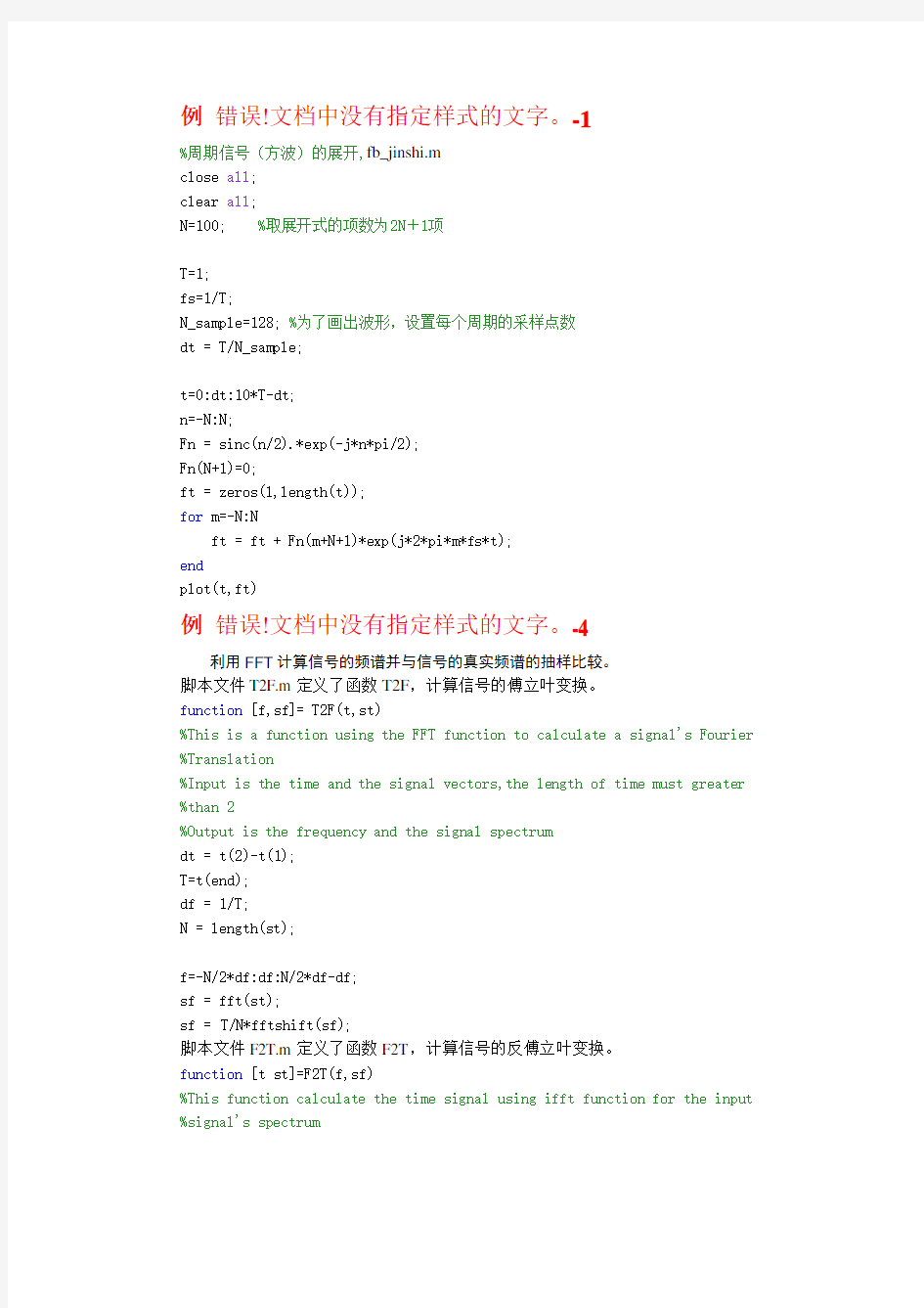
例错误!文档中没有指定样式的文字。-4
利用FFT计算信号的频谱并与信号的真实频谱的抽样比较。
脚本文件T2F.m定义了函数T2F,计算信号的傅立叶变换。
function [f,sf]= T2F(t,st)
%This is a function using the FFT function to calculate a signal's Fourier %Translation
%Input is the time and the signal vectors,the length of time must greater %than 2
%Output is the frequency and the signal spectrum
dt = t(2)-t(1);
T=t(end);
df = 1/T;
N = length(st);
f=-N/2*df:df:N/2*df-df;
sf = fft(st);
sf = T/N*fftshift(sf);
脚本文件F2T.m定义了函数F2T,计算信号的反傅立叶变换。
function [t st]=F2T(f,sf)
%This function calculate the time signal using ifft function for the input %signal's spectrum
df = f(2)-f(1);
Fmx = ( f(end)-f(1) +df);
dt = 1/Fmx;
N = length(sf);
T = dt*N;
%t=-T/2:dt:T/2-dt;
t = 0:dt:T-dt;
sff = fftshift(sf);
st = Fmx*ifft(sff);
另写脚本文件fb_spec.m如下:
%方波的傅氏变换, fb_spec.m
clear all;close all;
T=1;
N_sample = 128;
dt=T/N_sample;
t=0:dt:T-dt;
st=[ones(1,N_sample/2), -ones(1,N_sample/2)]; %方波一个周期
subplot(211);
plot(t,st);
axis([0 1 -2 2]);
xlabel('t'); ylabel('s(t)');
subplot(212);
[f sf]=T2F(t,st); %方波频谱
plot(f,abs(sf)); hold on;
axis([-10 10 0 1]);
xlabel('f');ylabel('|S(f)|');
%根据傅氏变换计算得到的信号频谱相应位置的抽样值
sff= T^2*j*pi*f*0.5.*exp(-j*2*pi*f*T).*sinc(f*T*0.5).*sinc(f*T*0.5);
plot(f,abs(sff),'r-')
例错误!文档中没有指定样式的文字。-5
%信号的能量计算或功率计算,sig_pow.m
clear all;
close all;
dt = 0.01;
t = 0:dt:5;
s1 = exp(-5*t).*cos(20*pi*t);
s2 = cos(20*pi*t);
E1 = sum(s1.*s1)*dt; %s1(t)的信号能量
P2 = sum(s2.*s2)*dt/(length(t)*dt); %s2(t)的信号功率s
[f1 s1f]= T2F(t,s1);
[f2 s2f]= T2F(t,s2);
df = f1(2)-f1(1);
E1_f = sum(abs(s1f).^2)*df; %s1(t)的能量,用频域方式计算
df = f2(2)-f2(1);
T = t(end);
P2_f = sum(abs(s2f).^2)*df/T; %s2(t)的功率,用频域方式计算
figure(1)
subplot(211)
plot(t,s1);
xlabel('t'); ylabel('s1(t)');
subplot(212)
plot(t,s2)
xlabel('t'); ylabel('s2(t)');
例错误!文档中没有指定样式的文字。-6
%方波的傅氏变换,sig_band.m
clear all;
close all;
T=1;
N_sample = 128;
dt=1/N_sample;
t=0:dt:T-dt;
st=[ones(1,N_sample/2) -ones(1,N_sample/2)];
df=0.1/T;
Fx = 1/dt;
f=-Fx:df:Fx-df;
%根据傅氏变换计算得到的信号频谱
sff= T^2*j*pi*f*0.5.*exp(-j*2*pi*f*T).*sinc(f*T*0.5).*sinc(f*T*0.5);
plot(f,abs(sff),'r-')
axis([-10 10 0 1]);
hold on;
sf_max = max(abs(sff));
line([f(1) f(end)],[sf_max sf_max]);
line([f(1) f(end)],[sf_max/sqrt(2) sf_max/sqrt(2)]); %交点处为信号功率下降3dB处Bw_eq = sum(abs(sff).^2)*df/T/sf_max.^2; %信号的等效带宽
例错误!文档中没有指定样式的文字。-7
%带通信号经过带通系统的等效基带表示,sig_bandpass.m
clear all;
close all;
dt = 0.01;
t = 0:dt:5;
s1 = exp(-t).*cos(20*pi*t); %输入信号
[f1 s1f]= T2F(t,s1); %输入信号的频谱
s1_lowpass = hilbert(s1).*exp(-j*2*pi*10*t); %输入信号的等效基带信号[f2 s2f]=T2F(t,s1_lowpass); %输入等效基带信号的频谱
h2f = zeros(1,length(s2f));
[a b]=find( abs(s1f)==max(abs(s1f)) ); %找到带通信号的中心频率
h2f( 201-25:201+25 )= 1;
h2f( 301-25:301+25) = 1;
h2f = h2f.*exp(-j*2*pi*f2); %加入线性相位,
[t1 h1] = F2T(f2,h2f); %带通系统的冲激响应
h1_lowpass = hilbert(h1).*exp(-j*2*pi*10*t1); %等效基带系统的冲激响应
figure(1)
subplot(521);
plot(t,s1);
xlabel('t'); ylabel('s1(t)'); title('带通信号');
subplot(523);
plot(f1,abs(s1f));
xlabel('f'); ylabel('|S1(f)|'); title('带通信号幅度谱');
subplot(522)
plot(t,real(s1_lowpass));
xlabel('t');ylabel('Re[s_l(t)]');title('等效基带信号的实部');
subplot(524)
plot(f2,abs(s2f));
xlabel('f');ylabel('|S_l(f)|');title('等效基带信号的幅度谱');
%画带通系统及其等效基带的图
subplot(525)
plot(f2,abs(h2f));
xlabel('f');ylabel('|H(f)|');title('带通系统的传输响应幅度谱'); subplot(527)
plot(t1,h1);
xlabel('t');ylabel('h(t)');title('带通系统的冲激响应');
subplot(526)
[f3 hlf]=T2F(t1,h1_lowpass);
plot(f3,abs(hlf));
xlabel('f');ylabel('|H_l(f)|');title('带通系统的等效基带幅度谱');
subplot(528)
plot(t1,h1_lowpass);
xlabel('t');ylabel('h_l(t)');title('带通系统的等效基带冲激响应');
%画出带通信号经过带通系统的响应及等效基带信号经过等效基带系统的响应
tt = 0:dt:t1(end)+t(end);
yt = conv(s1,h1);
subplot(529)
plot(tt,yt);
xlabel('t');ylabel('y(t)');title('带通信号与带通系统响应的卷积')
ytl = conv(s1_lowpass,h1_lowpass).*exp(j*2*pi*10*tt);
subplot(5,2,10)
plot(tt,real(yt));
xlabel('t');ylabel('y_l(t)cos(20*pi*t');
title('等效基带与等效基带系统响应的卷积×中心频率载波')
例3-6
%例:窄带高斯过程,文件 zdpw.m
clear all; close all;
N0=1; %双边功率谱密度
fc=10; %中心频率
B=1; %带宽
dt=0.01;
T=100;
t=0:dt:T-dt;
%产生功率为N0*B的高斯白噪声
P = N0*B;
st = sqrt(P)*randn(1,length(t));
%将上述白噪声经过窄带带通系统,
[f,sf] = T2F(t,st); %高斯信号频谱
figure(1)
plot(f,abs(sf)); %高斯信号的幅频特性
[tt gt]=bpf(f,sf,fc-B/2,fc+B/2); %高斯信号经过带通系统
glt = hilbert(real(gt)); %窄带信号的解析信号,调用hilbert函数得到解析信号glt = glt.*exp(-j*2*pi*fc*tt);
[ff,glf]=T2F( tt, glt );
figure(2)
plot(ff,abs(glf));
xlabel('频率(Hz)'); ylabel('窄带高斯过程样本的幅频特性')
figure(3)
subplot(411);
plot(tt,real(gt));
title('窄带高斯过程样本')
subplot(412)
plot(tt,real(glt).*cos(2*pi*fc*tt)-imag(glt).*sin(2*pi*fc*tt))
title('由等效基带重构的窄带高斯过程样本')
subplot(413)
plot(tt,real(glt));
title('窄带高斯过程样本的同相分量')
subplot(414)
plot(tt,imag(glt));
xlabel('时间t(秒)'); title('窄带高斯过程样本的正交分量')
%求窄带高斯信号功率;注:由于样本的功率近似等于随机过程的功率,因此可能出现一些偏差
P_gt=sum(real(gt).^2)/T;
P_glt_real = sum(real(glt).^2)/T;
P_glt_imag = sum(imag(glt).^2)/T;
%验证窄带高斯过程的同相分量、正交分量的正交性
a = real(glt)*(imag(glt))'/T;
用到的子函数
function [t,st]=bpf(f,sf,B1,B2)
%This function filter an input at frequency domain by an ideal bandpass filter %Inputs:
% f: frequency samples
% sf: input data spectrum samples
% B1: bandpass's lower frequency
% B2: bandpass's higher frequency
%Outputs:
% t: frequency samples
% st: output data's time samples
df = f(2)-f(1);
T = 1/df;
hf = zeros(1,length(f));
bf = [floor( B1/df ): floor( B2/df )] ;
bf1 = floor( length(f)/2 ) + bf;
bf2 = floor( length(f)/2 ) - bf;
hf(bf1)=1/sqrt(2*(B2-B1));
hf(bf2)=1/sqrt(2*(B2-B1));
yf=hf.*sf.*exp(-j*2*pi*f*0.1*T);
[t,st]=F2T(f,yf);
例4-1
%显示模拟调制的波形及解调方法DSB,文件mdsb.m %信源
close all;
clear all;
dt = 0.001; %时间采样间隔
fm=1; %信源最高频率
fc=10; %载波中心频率
T=5; %信号时长
t = 0:dt:T;
mt = sqrt(2)*cos(2*pi*fm*t); %信源
%N0 = 0.01; %白噪单边功率谱密度
%DSB modulation
s_dsb = mt.*cos(2*pi*fc*t);
B=2*fm;
%noise = noise_nb(fc,B,N0,t);
%s_dsb=s_dsb+noise;
figure(1)
subplot(311)
plot(t,s_dsb);hold on; %画出DSB信号波形plot(t,mt,'r--'); %标示mt的波形
title('DSB调制信号');
xlabel('t');
%DSB demodulation
rt = s_dsb.*cos(2*pi*fc*t);
rt = rt-mean(rt);
[f,rf] = T2F(t,rt);
[t,rt] = lpf(f,rf,2*fm);
subplot(312)
plot(t,rt); hold on;
plot(t,mt/2,'r--');
title('相干解调后的信号波形与输入信号的比较'); xlabel('t')
subplot(313)
[f,sf]=T2F(t,s_dsb);
psf = (abs(sf).^2)/T;
plot(f,psf);
axis([-2*fc 2*fc 0 max(psf)]);
title('DSB信号功率谱');
xlabel('f');
function [t st]=lpf(f,sf,B)
%This function filter an input data using a lowpass filter %Inputs: f: frequency samples
% sf: input data spectrum samples
% B: lowpass's bandwidth with a rectangle lowpass
%Outputs: t: time samples
% st: output data's time samples
df = f(2)-f(1);
T = 1/df;
hf = zeros(1,length(f));
bf = [-floor( B/df ): floor( B/df )] + floor( length(f)/2 ); hf(bf)=1;
yf=hf.*sf;
[t,st]=F2T(f,yf);
st = real(st);
例4-2
%显示模拟调制的波形及解调方法AM,文件mam.m
%信源
close all;
clear all;
dt = 0.001; %时间采样间隔
fm=1; %信源最高频率
fc=10; %载波中心频率
T=5; %信号时长
t = 0:dt:T;
mt = sqrt(2)*cos(2*pi*fm*t); %信源
%N0 = 0.01; %白噪单边功率谱密度
%AM modulation
A=2;
s_am = (A+mt).*cos(2*pi*fc*t);
B = 2*fm; %带通滤波器带宽
%noise = noise_nb(fc,B,N0,t); %窄带高斯噪声产生
%s_am = s_am + noise;
figure(1)
subplot(311)
plot(t,s_am);hold on; %画出AM信号波形
plot(t,A+mt,'r--'); %标示AM的包络
title('AM调制信号及其包络');
xlabel('t');
%AM demodulation
rt = s_am.*cos(2*pi*fc*t); %相干解调
rt = rt-mean(rt);
[f,rf] = T2F(t,rt);
[t,rt] = lpf(f,rf,2*fm); %低通滤波
subplot(312)
plot(t,rt); hold on;
plot(t,mt/2,'r--');
title('相干解调后的信号波形与输入信号的比较'); xlabel('t')
subplot(313)
[f,sf]=T2F(t,s_am);
psf = (abs(sf).^2)/T;
plot(f,psf);
axis([-2*fc 2*fc 0 max(psf)]);
title('AM信号功率谱');
xlabel('f');
例4-3
%显示模拟调制的波形及解调方法SSB,文件mssb.m
%信源
close all;
clear all;
dt = 0.001; %时间采样间隔
fm=1; %信源最高频率
fc=10; %载波中心频率
T=5; %信号时长
t = 0:dt:T;
mt = sqrt(2)*cos(2*pi*fm*t); %信源
%N0 = 0.01; %白噪单边功率谱密度
%SSB modulation
s_ssb = real( hilbert(mt).*exp(j*2*pi*fc*t) ); B=fm;
%noise = noise_nb(fc,B,N0,t);
%s_ssb=s_ssb+noise;
figure(1)
subplot(311)
plot(t,s_ssb);hold on; %画出SSB信号波形plot(t,mt,'r--'); %标示mt的波形
title('SSB调制信号');
xlabel('t');
%SSB demodulation
rt = s_ssb.*cos(2*pi*fc*t);
rt = rt-mean(rt);
[f,rf] = T2F(t,rt);
[t,rt] = lpf(f,rf,2*fm);
subplot(312)
plot(t,rt); hold on;
plot(t,mt/2,'r--');
title('相干解调后的信号波形与输入信号的比较');
xlabel('t')
subplot(313)
[f,sf]=T2F(t,s_ssb);
psf = (abs(sf).^2)/T;
plot(f,psf);
axis([-2*fc 2*fc 0 max(psf)]);
title('SSB信号功率谱');
xlabel('f');
例4-4
%显示模拟调制的波形及解调方法VSB,文件mvsb.m
%信源
close all;
clear all;
dt = 0.001; %时间采样间隔
fm=5; %信源最高频率
fc=20; %载波中心频率
T=5; %信号时长
t = 0:dt:T;
mt = sqrt(2)*( cos(2*pi*fm*t)+sin(2*pi*0.5*fm*t) ); %信源%VSB modulation
s_vsb = mt.*cos(2*pi*fc*t);
B=1.2*fm;
[f,sf] = T2F(t,s_vsb);
[t,s_vsb] = vsbpf(f,sf,0.2*fm,1.2*fm,fc);
figure(1)
subplot(311)
plot(t,s_vsb);hold on; %画出VSB信号波形
plot(t,mt,'r--'); %标示mt的波形
title('VSB调制信号');
xlabel('t');
%VSB demodulation
rt = s_vsb.*cos(2*pi*fc*t);
[f,rf] = T2F(t,rt);
[t,rt] = lpf(f,rf,2*fm);
subplot(312)
plot(t,rt); hold on;
plot(t,mt/2,'r--');
title('相干解调后的信号波形与输入信号的比较');
xlabel('t')
subplot(313)
[f,sf]=T2F(t,s_vsb);
psf = (abs(sf).^2)/T;
plot(f,psf);
axis([-2*fc 2*fc 0 max(psf)]);
title('VSB信号功率谱');
xlabel('f');
function [t,st]=vsbpf(f,sf,B1,B2,fc)
%This function filter an input by an residual bandpass filter %Inputs: f: frequency samples
% sf: input data spectrum samples
% B1: residual bandwidth
% B2: highest freq of the basedband signal
%Outputs: t: frequency samples
% st: output data's time samples
df = f(2)-f(1);
T = 1/df;
hf = zeros(1,length(f));
bf1 = [floor( (fc-B1)/df ): floor( (fc+B1)/df )] ;
bf2 = [floor( (fc+B1)/df )+1: floor( (fc+B2)/df )];
f1 = bf1 + floor( length(f)/2 ) ;
f2 = bf2 + floor( length(f)/2 ) ;
stepf = 1/length(f1);
hf(f1)=0:stepf:1-stepf;
hf(f2)=1;
f3 = -bf1 + floor( length(f)/2 ) ;
f4 = -bf2 + floor( length(f)/2) ;
hf(f3)=0:stepf:(1-stepf);
hf(f4)=1;
yf=hf.*sf;
[t,st]=F2T(f,yf);
st = real(st);
例4-5
%显示模拟调制的波形及解调方法AM、DSB、SSB, %信源
close all;
clear all;
dt = 0.001;
fm=1;
fc=10;
t = 0:dt:5;
mt = sqrt(2)*cos(2*pi*fm*t);
N0 = 0.1;
%AM modulation
A=2;
s_am = (A+mt).*cos(2*pi*fc*t);
B = 2*fm;
noise = noise_nb(fc,B,N0,t);
s_am = s_am + noise;
figure(1)
subplot(321)
plot(t,s_am);hold on;
plot(t,A+mt,'r--');
%AM demodulation
rt = s_am.*cos(2*pi*fc*t);
rt = rt-mean(rt);
[f,rf] = T2F(t,rt);
[t,rt] = lpf(f,rf,2*fm);
title('AM信号');xlabel('t');
subplot(322)
plot(t,rt); hold on;
plot(t,mt/2,'r--');
title('AM解调信号');xlabel('t');
%DSB modulation
s_dsb = mt.*cos(2*pi*fc*t);
B=2*fm;
noise = noise_nb(fc,B,N0,t);
s_dsb=s_dsb+noise;
subplot(323)
plot(t,s_dsb);hold on;
plot(t,mt,'r--');
title('DSB信号');xlabel('t');
%DSB demodulation
rt = s_dsb.*cos(2*pi*fc*t);
rt = rt-mean(rt);
[f,rf] = T2F(t,rt);
[t,rt] = lpf(f,rf,2*fm);
subplot(324)
plot(t,rt); hold on;
plot(t,mt/2,'r--');
title('DSB解调信号');xlabel('t');
%SSB modulation
s_ssb = real( hilbert(mt).*exp(j*2*pi*fc*t) );
B=fm;
noise = noise_nb(fc,B,N0,t);
s_ssb=s_ssb+noise;
subplot(325)
plot(t,s_ssb);
title('SSB信号');xlabel('t');
%SSB demodulation
rt = s_ssb.*cos(2*pi*fc*t);
rt = rt-mean(rt);
[f,rf] = T2F(t,rt);
[t,rt] = lpf(f,rf,2*fm);
subplot(326)
plot(t,rt); hold on;
plot(t,mt/2,'r--');
title('SSB解调信号');xlabel('t');
function [out] = noise_nb(fc,B,N0,t)
%output the narrow band gaussian noise sample with single-sided power spectrum N0 %at carrier frequency equals fc and bandwidth euqals B
dt = t(2)-t(1);
Fmx = 1/dt;
n_len = length(t);
p = N0*Fmx;
rn = sqrt(p)*randn(1,n_len);
[f,rf] = T2F(t,rn);
[t,out] = bpf(f,rf,fc-B/2,fc+B/2);
%FM modulation and demodulation,mfm.m
clear all;
close all;
Kf = 5;
fc = 10;
T=5;
dt=0.001;
t = 0:dt:T;
%信源
fm= 1;
%mt = cos(2*pi*fm*t) + 1.5*sin(2*pi*0.3*fm*t); %信源信号
mt = cos(2*pi*fm*t); %信源信号
%FM 调制
A = sqrt(2);
%mti = 1/2/pi/fm*sin(2*pi*fm*t) -3/4/pi/0.3/fm*cos(2*pi*0.3*fm*t); %mt的积分函数
mti = 1/2/pi/fm*sin(2*pi*fm*t) ; %mt的积分函数
st = A*cos(2*pi*fc*t + 2*pi*Kf*mti);
figure(1)
subplot(311);
plot(t,st); hold on;
plot(t,mt,'r--');
xlabel('t');ylabel('调频信号')
subplot(312)
[f sf] = T2F(t,st);
plot(f, abs(sf));
axis([-25 25 0 3])
xlabel('f');ylabel('调频信号幅度谱')
%FM 解调
for k=1:length(st)-1
rt(k) = (st(k+1)-st(k))/dt;
end
rt(length(st))=0;
subplot(313)
plot(t,rt); hold on;
plot(t,A*2*pi*Kf*mt+A*2*pi*fc,'r--');
xlabel('t');ylabel('调频信号微分后包络')
%数字基带信号的功率谱密度 digit_baseband.m
clear all; close all;
Ts=1;
N_sample = 8; %每个码元的抽样点数
dt = Ts/N_sample; %抽样时间间隔
N = 1000; %码元数
t = 0:dt:(N*N_sample-1)*dt;
gt1 = ones(1,N_sample); %NRZ非归零波形
gt2 = ones(1,N_sample/2); %RZ归零波形
gt2 = [gt2 zeros(1,N_sample/2)];
mt3 = sinc((t-5)/Ts); % sin(pi*t/Ts)/(pi*t/Ts)波形,截段取10个码元gt3 = mt3(1:10*N_sample);
d = ( sign( randn(1,N) ) +1 )/2;
data = sigexpand(d,N_sample); %对序列间隔插入N_sample-1个0
st1 = conv(data,gt1); %Matlab自带卷积函数
st2 = conv(data,gt2);
d = 2*d-1; %变成双极性序列
data= sigexpand(d,N_sample);
st3 = conv(data,gt3);
[f,st1f] = T2F(t,[st1(1:length(t))]);
[f,st2f] = T2F(t,[st2(1:length(t))]);
[f,st3f] = T2F(t,[st3(1:length(t))]);
figure(1)
subplot(321)
plot(t,[st1(1:length(t))] );grid
axis([0 20 -1.5 1.5]);ylabel('单极性NRZ波形');
subplot(322);
plot(f,10*log10(abs(st1f).^2/T) );grid
axis([-5 5 -40 10]); ylabel('单极性NRZ功率谱密度(dB/Hz)');
subplot(323)
plot(t,[st2(1:length(t))] );
axis([0 20 -1.5 1.5]);grid
ylabel('单极性RZ波形');
subplot(324)
plot(f,10*log10(abs(st2f).^2/T));
axis([-5 5 -40 10]);grid
ylabel('单极性RZ功率谱密度(dB/Hz)');
subplot(325)
plot(t-5,[st3(1:length(t))] );
axis([0 20 -2 2]);grid
ylabel('双极性sinc波形');xlabel('t/Ts');
subplot(326)
plot(f,10*log10(abs(st3f).^2/T));
axis([-5 5 -40 10]);grid
ylabel('sinc波形功率谱密度(dB/Hz)');xlabel('f*Ts');
function [out]=sigexpand(d,M)
%将输入的序列扩展成间隔为N-1个0的序列
N = length(d);
out = zeros(M,N);
out(1,:) = d;
out = reshape(out,1,M*N);
例5-2
%数字基带信号接收示意 digit_receive.m
clear all;
close all;
N =100;
N_sample=8; %每码元抽样点数
Ts=1;
dt = Ts/N_sample;
t=0:dt:(N*N_sample-1)*dt;
gt = ones(1,N_sample); %数字基带波形
d = sign(randn(1,N)); %输入数字序列
a = sigexpand(d,N_sample);
st = conv(a,gt); %数字基带信号
ht1 = gt;
rt1 = conv(st,ht1);
ht2 = 5*sinc(5*(t-5)/Ts);
rt2 = conv(st,ht2);
figure(1)
subplot(321)
plot( t,st(1:length(t)) );
axis([0 20 -1.5 1.5]); ylabel('输入双极性NRZ数字基带波形'); subplot(322)
stem( t,a);
axis([0 20 -1.5 1.5]); ylabel('输入数字序列')
subplot(323)
plot( t,[0 rt1(1:length(t)-1)]/8 );
axis([0 20 -1.5 1.5]);ylabel('方波滤波后输出');
subplot(324)
dd = rt1(N_sample:N_sample:end);
ddd= sigexpand(dd,N_sample);
stem( t,ddd(1:length(t))/8 );
axis([0 20 -1.5 1.5]);ylabel('方波滤波后抽样输出');
subplot(325)
plot(t-5, [0 rt2(1:length(t)-1)]/8 );
axis([0 20 -1.5 1.5]);
xlabel('t/Ts'); ylabel('理想低通滤波后输出');
subplot(326)
dd = rt2(N_sample-1:N_sample:end);
ddd=sigexpand(dd,N_sample);
stem( t-5,ddd(1:length(t))/8 );
axis([0 20 -1.5 1.5]);
xlabel('t/Ts'); ylabel('理想低通滤波后抽样输出');
例5-7
%部分响应信号眼图示意,pres.m
clear all; close all;
Ts=1;
N_sample=16;
eye_num = 11;
N_data=1000;
dt = Ts/N_sample;
t = -5*Ts:dt:5*Ts;
%产生双极性数字信号
d = sign(randn(1,N_data));
dd= sigexpand(d,N_sample);
%部分响应系统冲击响应
ht = sinc((t+eps)/Ts)./(1- (t+eps)./Ts);
ht( 6*N_sample+1 ) = 1;
st = conv(dd,ht);
tt = -5*Ts:dt:(N_data+5)*N_sample*dt-dt;
figure(1)
subplot(211);
plot(tt,st);
axis([0 20 -3 3]);xlabel('t/Ts');ylabel('部分响应基带信号'); subplot(212)
%画眼图
ss=zeros(1,eye_num*N_sample);
ttt = 0:dt:eye_num*N_sample*dt-dt;
for k=5:50
ss = st(k*N_sample+1:(k+eye_num)*N_sample);
drawnow;
plot(ttt,ss); hold on;
end
%plot(ttt,ss);
xlabel('t/Ts');ylabel('部分响应信号眼图');
例6-1
%2ASK,2PSK,文件名binarymod.m
clear all;
close all;
A=1;
fc = 2; %2Hz;
N_sample = 8;
N = 500; %码元数
Ts = 1; %1 baud/s
dt = Ts/fc/N_sample; %波形采样间隔
t = 0:dt:N*Ts-dt;
Lt = length(t);
%产生二进制信源
d = sign(randn(1,N));
dd = sigexpand((d+1)/2,fc*N_sample);
gt = ones(1,fc*N_sample); %NRZ波形
figure(1)
subplot(221); %输入NRZ信号波形(单极性)
d_NRZ = conv(dd,gt);
plot(t,d_NRZ(1:length(t)));
axis([0 10 0 1.2]); ylabel('输入信号');
subplot(222); %输入NRZ频谱
[f,d_NRZf]=T2F( t,d_NRZ(1:length(t)) );
plot(f,10*log10(abs(d_NRZf).^2/T));
axis([-2 2 -50 10]);ylabel('输入信号功率谱密度(dB/Hz)');
%2ASK信号
ht = A*cos(2*pi*fc*t);
s_2ask = d_NRZ(1:Lt).*ht;
subplot(223)
plot(t,s_2ask);
axis([0 10 -1.2 1.2]); ylabel('2ASK');
[f,s_2askf]=T2F(t,s_2ask );
subplot(224)
plot(f,10*log10(abs(s_2askf).^2/T));
axis([-fc-4 fc+4 -50 10]);ylabel('2ASK功率谱密度(dB/Hz)');
figure(2)
%2PSK信号
d_2psk = 2*d_NRZ-1;
s_2psk = d_2psk(1:Lt).*ht;
subplot(221)
plot(t,s_2psk);
axis([0 10 -1.2 1.2]); ylabel('2PSK');
subplot(222)
[f,s_2pskf] = T2F(t,s_2psk);
plot( f,10*log10(abs(s_2pskf).^2/T) );
axis([-fc-4 fc+4 -50 10]);ylabel('2PSK功率谱密度(dB/Hz)');
% 2FSK
% s_2fsk = Acos(2*pi*fc*t + int(2*d_NRZ-1) );
sd_2fsk = 2*d_NRZ-1;
s_2fsk = A*cos(2*pi*fc*t + 2*pi*sd_2fsk(1:length(t)).*t );
subplot(223)
plot(t,s_2fsk);
axis([0 10 -1.2 1.2]);xlabel('t'); ylabel('2FSK')
subplot(224)
[f,s_2fskf] = T2F(t,s_2fsk);
plot(f,10*log10(abs(s_2fskf).^2/T));
axis([-fc-4 fc+4 -50 10]);xlabel('f');ylabel('2FSK功率谱密度(dB/Hz)');
例6-3
%QPSK & OQPSK
clear all;
close all;
M = 4;
Ts= 1;
fc= 10;
N_sample = 16;
N_num = 100;
dt = 1/fc/N_sample;
t = 0:dt:N_num*Ts-dt;
T = dt*length(t);
py1f = zeros(1,length(t)); %功率谱密度1
py2f = zeros(1,length(t)); %功率谱密度2
for PL=1:100 %输入100段N_num个码字的波形,为了使功率谱密度看起来更加平滑,%可以取这100段信号功率谱密度的平均
d1 = sign(randn(1,N_num));
d2 = sign(randn(1,N_num));
gt = ones(1,fc*N_sample);
%QPSK调制
s1 = sigexpand(d1,fc*N_sample);
s2 = sigexpand(d2,fc*N_sample);
b1 = conv(s1,gt);
b2 = conv(s2,gt);
s1 = b1(1:length(s1));
s2 = b2(1:length(s2));
st_qpsk = s1.*cos(2*pi*fc*t) - s2.*sin(2*pi*fc*t);
s2_delay= [-ones(1,N_sample*fc/2) s2(1:end-N_sample*fc/2)];
st_oqpsk= s1.*cos(2*pi*fc*t) - s2_delay.*sin(2*pi*fc*t);
%经过带通后,再经过非线性电路
[f y1f] = T2F(t,st_qpsk);
[f y2f] = T2F(t,st_oqpsk);
[t y1] = bpf(f,y1f,fc-1/Ts,fc+1/Ts);
[t y2] = bpf(f,y2f,fc-1/Ts,fc+1/Ts);
subplot(221);