The Exciting Star of the Berkeley 59Cepheus OB4 Complex and Other Chance Variable Star Disc

2020年广东省中小学生天文知识竞赛试题（低年组）注意事项：1、本卷为闭卷考试，请答卷人按照自己的真实水平独立完成。

2、选择题全部为单项选择，考生直接在试题页面中点选一个最接近正确的答案，答错不扣分。

3、总分100分，每题2分，考试时间100分钟。

4、本场考试允许使用不具编程功能的计算器。

5、考试过程中不得切出考试页面，否则平台将自动收卷。

6、比赛结果将在广东天文学会网站和微信公众号公布。

_______________________________________________________________________________________________ Part 1. 天文热点1. 我国首个自主发射的火星探测器“天问一号”计划于何时入轨火星？ BA. 2020年12月底左右B. 2021年2月底左右C. 2021年5月中左右D. 2022年7月底左右2. 我国嫦娥五号探测器在今年何时发射升空？ CA. 12月24日B. 12月7日C. 11月24日D. 11月28日3. 2020年的诺贝尔物理学奖分别颁发给罗杰·彭罗斯、莱因哈特·根策尔和安德烈娅·盖兹。

其中彭罗斯获奖的理由是“发现黑洞形成是广义相对论的一个预言”，那根策尔和盖兹获奖的理由是？ AA. 发现银河系中心的超大质量致密天体B. 发现第一颗环绕类太阳恒星运动的系外行星C. 验证了引力波的存在D. 发现了一种测量宇宙大尺度结构的探针4. 以下哪所高校在今年正式成立天文系？ DA. 香港科技大学B. 贵州大学C. 中山大学D. 广州大学5. 今年7月，一颗“黑马”彗星亮度达到2等以上，吸引了很多爱好者拍摄。

这颗彗星是？CA. C/2019 Y4 (ATLAS)B. C/2020 F8 (SWAN)C. C/2020 F3（NEOWISE）D. C/2019 U6 (Lemmon)6. 关于今年6月21日的日环食，下列哪个地点位于环食带之外？ BA. 纳木错B. 武汉C. 厦门D. 泸州7. 今年4月24日是我国首个人造卫星“东方红一号”成功发射_______周年。

高一地球与宇宙探索英语阅读理解25题1<背景文章>The Earth is a complex and fascinating planet. It is composed of several layers. The outermost layer is the crust. The crust is relatively thin compared to the other layers. It is made up of different types of rocks and minerals.The mantle lies beneath the crust. It is much thicker and hotter than the crust. The mantle is made up of solid rock that can flow very slowly over long periods of time.The core is the innermost layer of the Earth. It is divided into two parts: the outer core and the inner core. The outer core is liquid and mainly composed of iron and nickel. The inner core is solid and also made up of iron and nickel.The Earth's surface is constantly changing due to geological processes such as plate tectonics. Plate tectonics is the movement of large sections of the Earth's crust. These plates can move apart, come together, or slide past each other.V olcanoes and earthquakes are common features on the Earth's surface. V olcanoes occur when magma from deep within the Earth erupts onto the surface. Earthquakes are caused by the movement of tectonicplates.1. The outermost layer of the Earth is called the ___.A. mantleB. coreC. crustD. magma答案：C。

【课⽂】 First listen and then answer the following question. 听录⾳，然后回答以下问题。

What does the 'uniquely rational way' for us to communicate with other intelligent beings in space depend on? We must conclude from the work of those who have studied the origin of life, that given a planet only approximately like our own, life is almost certain to start. Of all the planets in our solar system, we ware now pretty certain the Earth is the only one on which life can survive. Mars is too dry and poor in oxygen, Venus far too hot, and so is Mercury, and the outer planets have temperatures near absolute zero and hydrogen-dominated atmospheres. But other suns, start as the astronomers call them, are bound to have planets like our own, and as is the number of stars in the universe is so vast, this possibility becomes virtual certainty. There are one hundred thousand million starts in our own Milky Way alone, and then there are three thousand million other Milky Ways, or galaxies, in the universe. So the number of the stars that we know exist is now estimated at about 300 million million million. Although perhaps only 1 per cent of the life that has started somewhere will develop into highly complex and intelligent patterns, so vast is the number of planets, that intelligent life is bound to be a natural part of the universe. If then we are so certain that other intelligent life exists in the universe, why have we had no visitors from outer space yet? First of all, they may have come to this planet of ours thousands or millions of years ago, and found our then prevailing primitive state completely uninteresting to their own advanced knowledge. Professor Ronald Bracewell, a leading American radio astronomer, argued in Nature that such a superior civilization, on a visit to our own solar system, may have left an automatic messenger behind to await the possible awakening of an advanced civilization. Such a messenger, receiving our radio and television signals, might well re-transmit them back to its home-planet, although what impression any other civilization would thus get from us is best left unsaid. But here we come up against the most difficult of all obstacles to contact with people on other planets -- the astronomical distances which separate us. As a reasonable guess, they might, on an average, be 100 light years away. (A light year is the distance which light travels at 186,000 miles per second in one year, namely 6 million million miles.) Radio waves also travel at the speed of light, and assuming such an automatic messenger picked up our first broadcasts of the 1920's, the message to its home planet is barely halfway there. Similarly, our own present primitive chemical rockets, though good enough to orbit men, have no chance of transporting us to the nearest other star, four light years away, let alone distances of tens or hundreds of light years. Fortunately, there is a 'uniquely rational way' for us to communicate with other intelligent beings, as Walter Sullivan has put it in his excellent book, We Are not Alone. This depends on the precise radio frequency of the 21-cm wavelength, or 1420 megacycles per second. It is the natural frequency of emission of the hydrogen atoms in space and was discovered by us in 1951; it must be known to any kind of radio astronomer in the universe. Once the existence of this wave-length had been discovered, it was not long before its use as the uniquely recognizable broadcasting frequency for interstellar communication was suggested. Without something of this kind, searching for intelligences on other planets would be like trying to meet a friend in London without a pre-arranged rendezvous and absurdly wandering the streets in the hope of a chance encounter. ANTHONY MICHAELIS Are There Strangers in Space? from The Weekend Telegraph 【New words and expressions ⽣词和短语】 Mercury n. ⽔星 hydrogen n. 氢⽓ prevailing adj. 普遍的 radio astronomer 射电天⽅学家 uniquely adv. 地 rational adj. 合理的 radio frequency ⽆线电频率 cm n. 厘⽶ megacycle n. 兆周 emission n. 散发 intersteller adj.星际的 rendezvous n. 约会地点 【课⽂注释】 1.that given a planet only approximately like our own, life is almost certain to start 这是⼀个宾语从句，作动词conclude的宾语，其中given a planet...our own,过去分词短语作条件状语，given与if的意思相近，这个过去分词短语可译成“如果⼀个⾏星与我们所在的⾏星⼤致相同的话”。

《宇宙的奇迹》BBC和CCTV9纪录片合集，中英文字幕（包含文本）《宇宙的奇迹》有BBC和CCTV9制作的两个版本，每个版本都是分4集，在头条号《小智雅汇》用了8篇的篇幅，内容比较分散。

考虑到今日头条内容管理的扁平化，不便于数据的分类管理，为方便查看特制作此合集。

目录1（BBC制作，中英文字幕，英文语音，同时可查看中英文字幕的文本）宇宙的奇迹1 时间之箭(BBC纪录片，BrianCox讲述)宇宙的奇迹2 星尘(BBC纪录片，Brian Cox讲述)宇宙的奇迹3 引力(BBC纪录片，Brian Cox讲述)宇宙的奇迹4 信使(BBC纪录片，Brian Cox讲述)目录2（CCTV9制作，中文字幕，中文语音）宇宙的奇迹1 《命运》 Destiny(CCTV9纪录片)宇宙的奇迹2《星尘》Stardust(CCTV9纪录片)宇宙的奇迹3《引力》Gravity(CCTV9纪录片)宇宙的奇迹4《信使》(CCTV9纪录片)《宇宙的奇迹》（Wonders of the Universe）是BBC制作的一部纪录片，由Brian Cox布赖恩·考克斯教授带我们用物理学揭开种种宇宙奇迹的奥秘，阐释了人类和宇宙的深邃联系。

布赖恩·考克斯教授将带领我们穿越时间与空间，开始一段充满真知灼见而又令人兴奋的旅程：你会见证那个137亿年之久，930亿光年之广，1000亿个星系星罗棋布，而每个星系又包含着千亿、万亿颗恒星的无法想象的庞然大物。

我们把这个地方称作我们的宇宙。

它是如此广阔，如此复杂，几乎无法想象它能被人类所了解。

然而在过去的100年里，科学家们开始认识宇宙，开始将宇宙看似无穷无尽的复杂性化简成人类能够理解的知识，并总结出适用于所有时间、所有地点中的所有事物的自然规律。

由于这些规律适用于所有时间、所有地点中的所有事物，考克斯教授将会用地球上我们所熟悉的事物，为我们解释甚至带我们体验深空中那些宏大而深奥的现象，将那个变幻莫测、不可思议的宇宙带入活生生的现实。

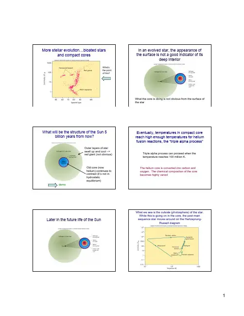
What the core is doing is not obvious from the surface of the starWhat will be the structure of the Sun 5billion years from now?Outer layers of starswell up and cool -->red giant (not obvious)Old core (nowhelium) continues tocontract (it’s not inhydrostaticequilibrium)demoEventually, temperatures in compact core reach high enough temperatures for helium fusion reactions, the “triple alpha process”Triple alpha process can proceed when thetemperature reaches 100 million K.Later in the future life of the SunRussell diagramnebulas, revealing the weird coressaw it during the field trip)As cores contract, the density goes to “astronomical” levels, matter acts in funnyways•Gas in this room, the “perfect gas law”PV=nRT. Pressure depends on both density and temperature•Extremely dense, “degenerate” gasPV=Kn. Pressure depends only on density•DemoThe contracted core reaches a new balance between gravity and degenerategas pressureWhat are the physical properties of theseobjects?Gas pressure Self gravityView from a spaceship in the Sirius system We know the white dwarfs must have the properties as described (we’re not makingthis up)There are many known examples of white dwarfs;they are a common phenomenon in the galaxy / WDCatalog/index.html。

Unit 5 Into the unknown 学案1．There is a profound charm in mystery. —Chatfield神秘事物具有深奥的魅力。

2．Nature is not governed except by obeying her. —Bacon自然不可驾驭，除非顺从她。

3．To be beautiful and to be calm is the ideal of nature. —Richard Jefferies美与宁静是自然的理想。

4．Mix a little mystery with everything，and the very mystery arouses veneration.任何事都掺一点神秘性，唯其神秘才引起崇拜。

5．He had lived long enough to know it is unwise to wish everything explained.长时期的生活经历足以使他懂得要想把一切都解释清楚是不明智的。

6．Man masters nature not by force but by understanding. —Bronwski人征服大自然不是凭力量，而是凭对它的认识。

The “Monster of Lake Tianchi” in the Changbai Mountains in Jilin Province，northeast China，is back in the news after several recent sightings.The director of a local tourist office，Meng Fanying，said the monster，which seemed to be black in color，was ten meters from the edge of the lake during the most recent sighting.“It jumped out of the water like a seal—about 200 people on Changbai's western peak saw it，”he said.“Although no one really got a clear look at the mysterious creature，Xue Junlin，a local photographer，claimed that its head looked like a horse.”In another recent sighting，a group of soldiers claim they saw an animal moving on the surface of the water.“It was greenish­black and had a round head with 10­centimeter horns”，one of the soldiers said.Mike Taylor，a university student in the study of prehistoric life forms for his Ph.D.，discovered a brand­new species of dinosaur，while conducting research at the Natural History Museum in the United Kingdom.This new species was identified as part of the sauropod family of dinosaurs.The sauropods were four-legged，vegetarian dinosaurs，with very long necks and tails，and relatively small skulls and brains.One of their most unusual characteristics was their nostrils，which were higher up in their head，almost near the eyes.So far，the sauropod bones have been found in every continent except Antarctica，and they are one of the longest living group of dinosaurs，spanning over 100 million years.This new species，named Xenoposeidon proneneukos，which means forward sloping，lived about 140 million years ago.Mike Taylor，who has spent five years studying sauropod vertebrae，immediately knew that this was the backbone of a sauropod.However，he had never seen one like this before.Further research proved this was indeed a new kind of sauropod.The bone，which had been discovered in the 1890s，had never been examined.[探究发现]1．Find out the main idea of the passage.Mike Taylor discovered a brand-new species of dinosaur.2．Find out the new dinosaur's most obvious characteristic.Nostril.3．Find out the time that the bone was discovered.In the 1890s.Ⅰ.匹配词义A．单词匹配()1.intrigue A．n.气旋；旋风()2.pyramid B．n.金字塔()3.astronomy C．n.衰败()4.tropical D．adj.来自热带的；产于热带的()5.cyclone E．v.(因奇特或神秘而)激起……的兴()6.downfall F．n.天文学()7.megadrought G．n.超级干旱[答案]1－5EBFDA6－7CGB．短语匹配()1.fall into ruin A．相当于()2.make a discovery B．收回()3.correspond to C．做出发现；发现()4.take back D．将……应用于……()5.apply...to... E．(因无人照料而)衰落，败落[答案]1－5ECABDⅡ.默写单词1．civilisation n．文明(社会)2．bury v. 将……埋在下面3．canal n. 运河4．ruin n. 残垣断壁，废墟5．abandon v. 离弃，逃离6．dismiss v. 拒绝考虑，否定7.expansion n. 扩大；增加Ⅰ.语境填词astronomy；dismiss；expansion；abandon；civilisation；was buried；canal；ruin The Victorians regarded the railways as bringing progress and civilisation．2．The truth has been buried in her memory since then.3．Astronomy is the scientific study of the sun，moon，stars，planets，etc. 4．A canal is a passage dug in the ground for boats and ships to travel along. 5．The old mill is now little more than a ruin．6．The cold weather forced us to abandon going out.7．I think we can safely dismiss their objections.8．Despite the difficulties the company is confident of further expansion．Ⅱ.语法填空之派生词1．Hunger and drought led to the collapse of Mayan civilisation(civilise)a millennium ago.2．The child was found abandoned(abandon)but unharmed.3．The buildings were in a ruinous (ruin)condition.4．Expansionism(expansion)was advocated by many British politicians in the late 19th century.5．There are no previous statistics for comparison(compare)．6．They questioned the accuracy(accurate)of the information in the file.7．The test can accurately (accurate)predict what a bigger explosion would do.8．Her dismissal(dismiss)of the threats seemed irresponsible.1．Although his theory has been dismissed by scholars，it shows how powerful the secrets of Ancient Maya civilisation are among people.虽然他的理论已经被学者们所否定，但它显示了古代玛雅文明的奥秘在人们心中是多么的有影响力。

全部图书(20)1. The Information 作者: James Gleick 出版社: Pantheon 2012添加2. The Wave Watcher's Companion作者: Pretor-Pinney, Ga vin 20113. Life Ascending 作者: Nick Lane 出版社: Profile Books 评语 : 20104. The Age of Wonder 作者: Richard Holmes 出版社: Pantheon 20095. 好奇年代 作者: [英]理查德·霍姆斯 出版社: 湖南科学技术出版社 20096. Six Degrees 作者: Mark Lynas 出版社: National Geographic20087. 撞上快乐作者: (美)丹尼尔.吉尔伯特出版社: 中信出版社20078. Electric Universe作者: David Bodanis出版社: Broadway20069. Critical Mass作者: Philip Ball出版社: Farrar, Straus and Giroux 200510. 万物简史作者: [美] 比尔·布莱森出版社: 接力出版社: 200411. 右手.左手作者: 麦克马纳斯出版社: 北京理工大学出版社200312. 果壳中的宇宙作者: [英] 史蒂芬·霍金出版社: 湖南科学技术出版社: 200213. Mapping the Deep作者: Kunzig, Robert出版社: W W Norton & Co Inc 200114. The Elegant Universe作者: Brian Greene出版社: Vintage Books200015. 数字情种作者: [美] 保罗·霍夫曼出版社: 上海科技教育出版社199916. 枪炮、病菌与钢铁作者: (美)贾雷德・戴蒙德出版社: 上海译文出版社199817. The Wisdom of the Bones作者: Alan Walker/Pat Shipman出版社: Vintage: 199718. 第三种猩猩作者: 杰拉德・戴蒙德出版社: 海南出版社199219. Wonderful Life作者: Stephen Jay Gould出版社: W. W. Norton & Company 199120. 皇帝新脑作者: 罗杰·彭罗斯出版社: 湖南科学技术出版社1990。

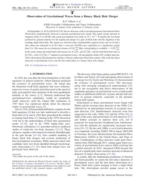
Observation of Gravitational Waves from a Binary Black Hole MergerB.P.Abbott et al.*(LIGO Scientific Collaboration and Virgo Collaboration)(Received21January2016;published11February2016)On September14,2015at09:50:45UTC the two detectors of the Laser Interferometer Gravitational-Wave Observatory simultaneously observed a transient gravitational-wave signal.The signal sweeps upwards in frequency from35to250Hz with a peak gravitational-wave strain of1.0×10−21.It matches the waveform predicted by general relativity for the inspiral and merger of a pair of black holes and the ringdown of the resulting single black hole.The signal was observed with a matched-filter signal-to-noise ratio of24and a false alarm rate estimated to be less than1event per203000years,equivalent to a significance greaterthan5.1σ.The source lies at a luminosity distance of410þ160−180Mpc corresponding to a redshift z¼0.09þ0.03−0.04.In the source frame,the initial black hole masses are36þ5−4M⊙and29þ4−4M⊙,and the final black hole mass is62þ4−4M⊙,with3.0þ0.5−0.5M⊙c2radiated in gravitational waves.All uncertainties define90%credible intervals.These observations demonstrate the existence of binary stellar-mass black hole systems.This is the first direct detection of gravitational waves and the first observation of a binary black hole merger.DOI:10.1103/PhysRevLett.116.061102I.INTRODUCTIONIn1916,the year after the final formulation of the field equations of general relativity,Albert Einstein predicted the existence of gravitational waves.He found that the linearized weak-field equations had wave solutions: transverse waves of spatial strain that travel at the speed of light,generated by time variations of the mass quadrupole moment of the source[1,2].Einstein understood that gravitational-wave amplitudes would be remarkably small;moreover,until the Chapel Hill conference in 1957there was significant debate about the physical reality of gravitational waves[3].Also in1916,Schwarzschild published a solution for the field equations[4]that was later understood to describe a black hole[5,6],and in1963Kerr generalized the solution to rotating black holes[7].Starting in the1970s theoretical work led to the understanding of black hole quasinormal modes[8–10],and in the1990s higher-order post-Newtonian calculations[11]preceded extensive analytical studies of relativistic two-body dynamics[12,13].These advances,together with numerical relativity breakthroughs in the past decade[14–16],have enabled modeling of binary black hole mergers and accurate predictions of their gravitational waveforms.While numerous black hole candidates have now been identified through electromag-netic observations[17–19],black hole mergers have not previously been observed.The discovery of the binary pulsar system PSR B1913þ16 by Hulse and Taylor[20]and subsequent observations of its energy loss by Taylor and Weisberg[21]demonstrated the existence of gravitational waves.This discovery, along with emerging astrophysical understanding[22], led to the recognition that direct observations of the amplitude and phase of gravitational waves would enable studies of additional relativistic systems and provide new tests of general relativity,especially in the dynamic strong-field regime.Experiments to detect gravitational waves began with Weber and his resonant mass detectors in the1960s[23], followed by an international network of cryogenic reso-nant detectors[24].Interferometric detectors were first suggested in the early1960s[25]and the1970s[26].A study of the noise and performance of such detectors[27], and further concepts to improve them[28],led to proposals for long-baseline broadband laser interferome-ters with the potential for significantly increased sensi-tivity[29–32].By the early2000s,a set of initial detectors was completed,including TAMA300in Japan,GEO600 in Germany,the Laser Interferometer Gravitational-Wave Observatory(LIGO)in the United States,and Virgo in binations of these detectors made joint obser-vations from2002through2011,setting upper limits on a variety of gravitational-wave sources while evolving into a global network.In2015,Advanced LIGO became the first of a significantly more sensitive network of advanced detectors to begin observations[33–36].A century after the fundamental predictions of Einstein and Schwarzschild,we report the first direct detection of gravitational waves and the first direct observation of a binary black hole system merging to form a single black hole.Our observations provide unique access to the*Full author list given at the end of the article.Published by the American Physical Society under the terms of the Creative Commons Attribution3.0License.Further distri-bution of this work must maintain attribution to the author(s)and the published article’s title,journal citation,and DOI.properties of space-time in the strong-field,high-velocity regime and confirm predictions of general relativity for the nonlinear dynamics of highly disturbed black holes.II.OBSERVATIONOn September14,2015at09:50:45UTC,the LIGO Hanford,W A,and Livingston,LA,observatories detected the coincident signal GW150914shown in Fig.1.The initial detection was made by low-latency searches for generic gravitational-wave transients[41]and was reported within three minutes of data acquisition[43].Subsequently, matched-filter analyses that use relativistic models of com-pact binary waveforms[44]recovered GW150914as the most significant event from each detector for the observa-tions reported here.Occurring within the10-msintersite FIG.1.The gravitational-wave event GW150914observed by the LIGO Hanford(H1,left column panels)and Livingston(L1,rightcolumn panels)detectors.Times are shown relative to September14,2015at09:50:45UTC.For visualization,all time series are filtered with a35–350Hz bandpass filter to suppress large fluctuations outside the detectors’most sensitive frequency band,and band-reject filters to remove the strong instrumental spectral lines seen in the Fig.3spectra.Top row,left:H1strain.Top row,right:L1strain.GW150914arrived first at L1and6.9þ0.5−0.4ms later at H1;for a visual comparison,the H1data are also shown,shifted in time by this amount and inverted(to account for the detectors’relative orientations).Second row:Gravitational-wave strain projected onto each detector in the35–350Hz band.Solid lines show a numerical relativity waveform for a system with parameters consistent with those recovered from GW150914[37,38]confirmed to99.9%by an independent calculation based on[15].Shaded areas show90%credible regions for two independent waveform reconstructions.One(dark gray)models the signal using binary black hole template waveforms [39].The other(light gray)does not use an astrophysical model,but instead calculates the strain signal as a linear combination of sine-Gaussian wavelets[40,41].These reconstructions have a94%overlap,as shown in[39].Third row:Residuals after subtracting the filtered numerical relativity waveform from the filtered detector time series.Bottom row:A time-frequency representation[42]of the strain data,showing the signal frequency increasing over time.propagation time,the events have a combined signal-to-noise ratio(SNR)of24[45].Only the LIGO detectors were observing at the time of GW150914.The Virgo detector was being upgraded, and GEO600,though not sufficiently sensitive to detect this event,was operating but not in observational mode.With only two detectors the source position is primarily determined by the relative arrival time and localized to an area of approximately600deg2(90% credible region)[39,46].The basic features of GW150914point to it being produced by the coalescence of two black holes—i.e., their orbital inspiral and merger,and subsequent final black hole ringdown.Over0.2s,the signal increases in frequency and amplitude in about8cycles from35to150Hz,where the amplitude reaches a maximum.The most plausible explanation for this evolution is the inspiral of two orbiting masses,m1and m2,due to gravitational-wave emission.At the lower frequencies,such evolution is characterized by the chirp mass[11]M¼ðm1m2Þ3=5121=5¼c3G596π−8=3f−11=3_f3=5;where f and_f are the observed frequency and its time derivative and G and c are the gravitational constant and speed of light.Estimating f and_f from the data in Fig.1, we obtain a chirp mass of M≃30M⊙,implying that the total mass M¼m1þm2is≳70M⊙in the detector frame. This bounds the sum of the Schwarzschild radii of thebinary components to2GM=c2≳210km.To reach an orbital frequency of75Hz(half the gravitational-wave frequency)the objects must have been very close and very compact;equal Newtonian point masses orbiting at this frequency would be only≃350km apart.A pair of neutron stars,while compact,would not have the required mass,while a black hole neutron star binary with the deduced chirp mass would have a very large total mass, and would thus merge at much lower frequency.This leaves black holes as the only known objects compact enough to reach an orbital frequency of75Hz without contact.Furthermore,the decay of the waveform after it peaks is consistent with the damped oscillations of a black hole relaxing to a final stationary Kerr configuration. Below,we present a general-relativistic analysis of GW150914;Fig.2shows the calculated waveform using the resulting source parameters.III.DETECTORSGravitational-wave astronomy exploits multiple,widely separated detectors to distinguish gravitational waves from local instrumental and environmental noise,to provide source sky localization,and to measure wave polarizations. The LIGO sites each operate a single Advanced LIGO detector[33],a modified Michelson interferometer(see Fig.3)that measures gravitational-wave strain as a differ-ence in length of its orthogonal arms.Each arm is formed by two mirrors,acting as test masses,separated by L x¼L y¼L¼4km.A passing gravitational wave effec-tively alters the arm lengths such that the measured difference isΔLðtÞ¼δL x−δL y¼hðtÞL,where h is the gravitational-wave strain amplitude projected onto the detector.This differential length variation alters the phase difference between the two light fields returning to the beam splitter,transmitting an optical signal proportional to the gravitational-wave strain to the output photodetector. To achieve sufficient sensitivity to measure gravitational waves,the detectors include several enhancements to the basic Michelson interferometer.First,each arm contains a resonant optical cavity,formed by its two test mass mirrors, that multiplies the effect of a gravitational wave on the light phase by a factor of300[48].Second,a partially trans-missive power-recycling mirror at the input provides addi-tional resonant buildup of the laser light in the interferometer as a whole[49,50]:20W of laser input is increased to700W incident on the beam splitter,which is further increased to 100kW circulating in each arm cavity.Third,a partially transmissive signal-recycling mirror at the outputoptimizes FIG. 2.Top:Estimated gravitational-wave strain amplitude from GW150914projected onto H1.This shows the full bandwidth of the waveforms,without the filtering used for Fig.1. The inset images show numerical relativity models of the black hole horizons as the black holes coalesce.Bottom:The Keplerian effective black hole separation in units of Schwarzschild radii (R S¼2GM=c2)and the effective relative velocity given by the post-Newtonian parameter v=c¼ðGMπf=c3Þ1=3,where f is the gravitational-wave frequency calculated with numerical relativity and M is the total mass(value from Table I).the gravitational-wave signal extraction by broadening the bandwidth of the arm cavities [51,52].The interferometer is illuminated with a 1064-nm wavelength Nd:Y AG laser,stabilized in amplitude,frequency,and beam geometry [53,54].The gravitational-wave signal is extracted at the output port using a homodyne readout [55].These interferometry techniques are designed to maxi-mize the conversion of strain to optical signal,thereby minimizing the impact of photon shot noise (the principal noise at high frequencies).High strain sensitivity also requires that the test masses have low displacement noise,which is achieved by isolating them from seismic noise (low frequencies)and designing them to have low thermal noise (intermediate frequencies).Each test mass is suspended as the final stage of a quadruple-pendulum system [56],supported by an active seismic isolation platform [57].These systems collectively provide more than 10orders of magnitude of isolation from ground motion for frequen-cies above 10Hz.Thermal noise is minimized by using low-mechanical-loss materials in the test masses and their suspensions:the test masses are 40-kg fused silica substrates with low-loss dielectric optical coatings [58,59],and are suspended with fused silica fibers from the stage above [60].To minimize additional noise sources,all components other than the laser source are mounted on vibration isolation stages in ultrahigh vacuum.To reduce optical phase fluctuations caused by Rayleigh scattering,the pressure in the 1.2-m diameter tubes containing the arm-cavity beams is maintained below 1μPa.Servo controls are used to hold the arm cavities on resonance [61]and maintain proper alignment of the optical components [62].The detector output is calibrated in strain by measuring its response to test mass motion induced by photon pressure from a modulated calibration laser beam [63].The calibration is established to an uncertainty (1σ)of less than 10%in amplitude and 10degrees in phase,and is continuously monitored with calibration laser excitations at selected frequencies.Two alternative methods are used to validate the absolute calibration,one referenced to the main laser wavelength and the other to a radio-frequencyoscillator(a)FIG.3.Simplified diagram of an Advanced LIGO detector (not to scale).A gravitational wave propagating orthogonally to the detector plane and linearly polarized parallel to the 4-km optical cavities will have the effect of lengthening one 4-km arm and shortening the other during one half-cycle of the wave;these length changes are reversed during the other half-cycle.The output photodetector records these differential cavity length variations.While a detector ’s directional response is maximal for this case,it is still significant for most other angles of incidence or polarizations (gravitational waves propagate freely through the Earth).Inset (a):Location and orientation of the LIGO detectors at Hanford,WA (H1)and Livingston,LA (L1).Inset (b):The instrument noise for each detector near the time of the signal detection;this is an amplitude spectral density,expressed in terms of equivalent gravitational-wave strain amplitude.The sensitivity is limited by photon shot noise at frequencies above 150Hz,and by a superposition of other noise sources at lower frequencies [47].Narrow-band features include calibration lines (33–38,330,and 1080Hz),vibrational modes of suspension fibers (500Hz and harmonics),and 60Hz electric power grid harmonics.[64].Additionally,the detector response to gravitational waves is tested by injecting simulated waveforms with the calibration laser.To monitor environmental disturbances and their influ-ence on the detectors,each observatory site is equipped with an array of sensors:seismometers,accelerometers, microphones,magnetometers,radio receivers,weather sensors,ac-power line monitors,and a cosmic-ray detector [65].Another∼105channels record the interferometer’s operating point and the state of the control systems.Data collection is synchronized to Global Positioning System (GPS)time to better than10μs[66].Timing accuracy is verified with an atomic clock and a secondary GPS receiver at each observatory site.In their most sensitive band,100–300Hz,the current LIGO detectors are3to5times more sensitive to strain than initial LIGO[67];at lower frequencies,the improvement is even greater,with more than ten times better sensitivity below60Hz.Because the detectors respond proportionally to gravitational-wave amplitude,at low redshift the volume of space to which they are sensitive increases as the cube of strain sensitivity.For binary black holes with masses similar to GW150914,the space-time volume surveyed by the observations reported here surpasses previous obser-vations by an order of magnitude[68].IV.DETECTOR VALIDATIONBoth detectors were in steady state operation for several hours around GW150914.All performance measures,in particular their average sensitivity and transient noise behavior,were typical of the full analysis period[69,70]. Exhaustive investigations of instrumental and environ-mental disturbances were performed,giving no evidence to suggest that GW150914could be an instrumental artifact [69].The detectors’susceptibility to environmental disturb-ances was quantified by measuring their response to spe-cially generated magnetic,radio-frequency,acoustic,and vibration excitations.These tests indicated that any external disturbance large enough to have caused the observed signal would have been clearly recorded by the array of environ-mental sensors.None of the environmental sensors recorded any disturbances that evolved in time and frequency like GW150914,and all environmental fluctuations during the second that contained GW150914were too small to account for more than6%of its strain amplitude.Special care was taken to search for long-range correlated disturbances that might produce nearly simultaneous signals at the two sites. No significant disturbances were found.The detector strain data exhibit non-Gaussian noise transients that arise from a variety of instrumental mecha-nisms.Many have distinct signatures,visible in auxiliary data channels that are not sensitive to gravitational waves; such instrumental transients are removed from our analyses [69].Any instrumental transients that remain in the data are accounted for in the estimated detector backgrounds described below.There is no evidence for instrumental transients that are temporally correlated between the two detectors.V.SEARCHESWe present the analysis of16days of coincident observations between the two LIGO detectors from September12to October20,2015.This is a subset of the data from Advanced LIGO’s first observational period that ended on January12,2016.GW150914is confidently detected by two different types of searches.One aims to recover signals from the coalescence of compact objects,using optimal matched filtering with waveforms predicted by general relativity. The other search targets a broad range of generic transient signals,with minimal assumptions about waveforms.These searches use independent methods,and their response to detector noise consists of different,uncorrelated,events. However,strong signals from binary black hole mergers are expected to be detected by both searches.Each search identifies candidate events that are detected at both observatories consistent with the intersite propa-gation time.Events are assigned a detection-statistic value that ranks their likelihood of being a gravitational-wave signal.The significance of a candidate event is determined by the search background—the rate at which detector noise produces events with a detection-statistic value equal to or higher than the candidate event.Estimating this back-ground is challenging for two reasons:the detector noise is nonstationary and non-Gaussian,so its properties must be empirically determined;and it is not possible to shield the detector from gravitational waves to directly measure a signal-free background.The specific procedure used to estimate the background is slightly different for the two searches,but both use a time-shift technique:the time stamps of one detector’s data are artificially shifted by an offset that is large compared to the intersite propagation time,and a new set of events is produced based on this time-shifted data set.For instrumental noise that is uncor-related between detectors this is an effective way to estimate the background.In this process a gravitational-wave signal in one detector may coincide with time-shifted noise transients in the other detector,thereby contributing to the background estimate.This leads to an overestimate of the noise background and therefore to a more conservative assessment of the significance of candidate events.The characteristics of non-Gaussian noise vary between different time-frequency regions.This means that the search backgrounds are not uniform across the space of signals being searched.To maximize sensitivity and provide a better estimate of event significance,the searches sort both their background estimates and their event candidates into differ-ent classes according to their time-frequency morphology. The significance of a candidate event is measured against the background of its class.To account for having searchedmultiple classes,this significance is decreased by a trials factor equal to the number of classes [71].A.Generic transient searchDesigned to operate without a specific waveform model,this search identifies coincident excess power in time-frequency representations of the detector strain data [43,72],for signal frequencies up to 1kHz and durations up to a few seconds.The search reconstructs signal waveforms consistent with a common gravitational-wave signal in both detectors using a multidetector maximum likelihood method.Each event is ranked according to the detection statistic ηc ¼ffiffiffiffiffiffiffiffiffiffiffiffiffiffiffiffiffiffiffiffiffiffiffiffiffiffiffiffiffiffiffiffiffiffiffi2E c =ð1þE n =E c Þp ,where E c is the dimensionless coherent signal energy obtained by cross-correlating the two reconstructed waveforms,and E n is the dimensionless residual noise energy after the reconstructed signal is subtracted from the data.The statistic ηc thus quantifies the SNR of the event and the consistency of the data between the two detectors.Based on their time-frequency morphology,the events are divided into three mutually exclusive search classes,as described in [41]:events with time-frequency morphology of known populations of noise transients (class C1),events with frequency that increases with time (class C3),and all remaining events (class C2).Detected with ηc ¼20.0,GW150914is the strongest event of the entire search.Consistent with its coalescence signal signature,it is found in the search class C3of events with increasing time-frequency evolution.Measured on a background equivalent to over 67400years of data and including a trials factor of 3to account for the search classes,its false alarm rate is lower than 1in 22500years.This corresponds to a probability <2×10−6of observing one or more noise events as strong as GW150914during the analysis time,equivalent to 4.6σ.The left panel of Fig.4shows the C3class results and background.The selection criteria that define the search class C3reduce the background by introducing a constraint on the signal morphology.In order to illustrate the significance of GW150914against a background of events with arbitrary shapes,we also show the results of a search that uses the same set of events as the one described above but without this constraint.Specifically,we use only two search classes:the C1class and the union of C2and C3classes (C 2þC 3).In this two-class search the GW150914event is found in the C 2þC 3class.The left panel of Fig.4shows the C 2þC 3class results and background.In the background of this class there are four events with ηc ≥32.1,yielding a false alarm rate for GW150914of 1in 8400years.This corresponds to a false alarm probability of 5×10−6equivalent to 4.4σ.FIG.4.Search results from the generic transient search (left)and the binary coalescence search (right).These histograms show the number of candidate events (orange markers)and the mean number of background events (black lines)in the search class where GW150914was found as a function of the search detection statistic and with a bin width of 0.2.The scales on the top give the significance of an event in Gaussian standard deviations based on the corresponding noise background.The significance of GW150914is greater than 5.1σand 4.6σfor the binary coalescence and the generic transient searches,respectively.Left:Along with the primary search (C3)we also show the results (blue markers)and background (green curve)for an alternative search that treats events independently of their frequency evolution (C 2þC 3).The classes C2and C3are defined in the text.Right:The tail in the black-line background of the binary coalescence search is due to random coincidences of GW150914in one detector with noise in the other detector.(This type of event is practically absent in the generic transient search background because they do not pass the time-frequency consistency requirements used in that search.)The purple curve is the background excluding those coincidences,which is used to assess the significance of the second strongest event.For robustness and validation,we also use other generic transient search algorithms[41].A different search[73]and a parameter estimation follow-up[74]detected GW150914 with consistent significance and signal parameters.B.Binary coalescence searchThis search targets gravitational-wave emission from binary systems with individual masses from1to99M⊙, total mass less than100M⊙,and dimensionless spins up to 0.99[44].To model systems with total mass larger than 4M⊙,we use the effective-one-body formalism[75],whichcombines results from the post-Newtonian approach [11,76]with results from black hole perturbation theory and numerical relativity.The waveform model[77,78] assumes that the spins of the merging objects are alignedwith the orbital angular momentum,but the resultingtemplates can,nonetheless,effectively recover systemswith misaligned spins in the parameter region ofGW150914[44].Approximately250000template wave-forms are used to cover this parameter space.The search calculates the matched-filter signal-to-noiseratioρðtÞfor each template in each detector and identifiesmaxima ofρðtÞwith respect to the time of arrival of the signal[79–81].For each maximum we calculate a chi-squared statisticχ2r to test whether the data in several differentfrequency bands are consistent with the matching template [82].Values ofχ2r near unity indicate that the signal is consistent with a coalescence.Ifχ2r is greater than unity,ρðtÞis reweighted asˆρ¼ρ=f½1þðχ2rÞ3 =2g1=6[83,84].The final step enforces coincidence between detectors by selectingevent pairs that occur within a15-ms window and come fromthe same template.The15-ms window is determined by the10-ms intersite propagation time plus5ms for uncertainty inarrival time of weak signals.We rank coincident events basedon the quadrature sumˆρc of theˆρfrom both detectors[45]. To produce background data for this search the SNR maxima of one detector are time shifted and a new set of coincident events is computed.Repeating this procedure ∼107times produces a noise background analysis time equivalent to608000years.To account for the search background noise varying acrossthe target signal space,candidate and background events aredivided into three search classes based on template length.The right panel of Fig.4shows the background for thesearch class of GW150914.The GW150914detection-statistic value ofˆρc¼23.6is larger than any background event,so only an upper bound can be placed on its false alarm rate.Across the three search classes this bound is1in 203000years.This translates to a false alarm probability <2×10−7,corresponding to5.1σ.A second,independent matched-filter analysis that uses adifferent method for estimating the significance of itsevents[85,86],also detected GW150914with identicalsignal parameters and consistent significance.When an event is confidently identified as a real gravitational-wave signal,as for GW150914,the back-ground used to determine the significance of other events is reestimated without the contribution of this event.This is the background distribution shown as a purple line in the right panel of Fig.4.Based on this,the second most significant event has a false alarm rate of1per2.3years and corresponding Poissonian false alarm probability of0.02. Waveform analysis of this event indicates that if it is astrophysical in origin it is also a binary black hole merger[44].VI.SOURCE DISCUSSIONThe matched-filter search is optimized for detecting signals,but it provides only approximate estimates of the source parameters.To refine them we use general relativity-based models[77,78,87,88],some of which include spin precession,and for each model perform a coherent Bayesian analysis to derive posterior distributions of the source parameters[89].The initial and final masses, final spin,distance,and redshift of the source are shown in Table I.The spin of the primary black hole is constrained to be<0.7(90%credible interval)indicating it is not maximally spinning,while the spin of the secondary is only weakly constrained.These source parameters are discussed in detail in[39].The parameter uncertainties include statistical errors and systematic errors from averaging the results of different waveform models.Using the fits to numerical simulations of binary black hole mergers in[92,93],we provide estimates of the mass and spin of the final black hole,the total energy radiated in gravitational waves,and the peak gravitational-wave luminosity[39].The estimated total energy radiated in gravitational waves is3.0þ0.5−0.5M⊙c2.The system reached apeak gravitational-wave luminosity of3.6þ0.5−0.4×1056erg=s,equivalent to200þ30−20M⊙c2=s.Several analyses have been performed to determine whether or not GW150914is consistent with a binary TABLE I.Source parameters for GW150914.We report median values with90%credible intervals that include statistical errors,and systematic errors from averaging the results of different waveform models.Masses are given in the source frame;to convert to the detector frame multiply by(1þz) [90].The source redshift assumes standard cosmology[91]. Primary black hole mass36þ5−4M⊙Secondary black hole mass29þ4−4M⊙Final black hole mass62þ4−4M⊙Final black hole spin0.67þ0.05−0.07 Luminosity distance410þ160−180MpcSource redshift z0.09þ0.03−0.04。

飞屋环游记（双语剧本注释版）田哥书斋（/）欢迎你推荐优秀藏品，共赏！[Movie Fan News presents: Spotlight on "Adventure"]spotlight: 聚光灯-Overtone: What you are now witnessing is footage never before seen by civilized humanity,witness: 目击 footage: 影片镜头 civilized: 文明的 humanity: 人类什么是现代没有看过的东西?A lost world in South America, lurking in the shadow of Majestic Paradise Fallslost: 消失的 South America: 南美洲 lurk: 潜伏 majestic: 宏伟的paradise: 天堂 falls: 瀑布在南美洲消失的国家看到天堂般的瀑布。

It's full of plants and animals undiscovered by science.full of: 充满 undiscovered: 未被发现的 science: 科学那里遍布着连科学家都未知的动植物。

Who would dare set foot on this inhospitable summit? Why, our subject today, Charles Muntz.dare: 敢 inhospitable: 格格不入的 summit: 高峰 subject: 主角有谁，胆敢闯入这处高高在上的胜境？我们今天主角Charles。

The beloved explorer lands his dirigible, "The Spirit of Adventure", into Hampshire,beloved:受喜爱的 land:使着陆 dirigible:飞船 spirit: 灵魂，精神adventure:冒险Hampshire: 新罕布什尔州这位备受喜爱的探险家，架着他那飞艇“探险精神号”，来到新罕布什尔州，this week, completing a year long expedition to the lost world.complete: 完成 expedition: 探险完成了他在迷失大陆上为期一年的考察。