
SAS/Graph实用基础教程(Gplot、Gchart)(2008-11-28 16:16:54)
标签:gplot gchart sas graph教育分类:Graph专题
An Introduction to the Simplicity and Power of SAS/Graph?
SAS/Graph实用基础教程(Gplot、Gchart)
原文地址:https://www.doczj.com/doc/e510230956.html,/proceedings/sugi30/262-30.pdf
转载请注明出处:https://www.doczj.com/doc/e510230956.html,/s/blog_5d3b177c0100bams.html
SAS/Graph太强大了,本文主要讲一些常用且功能强大的Graph相关的过程步。
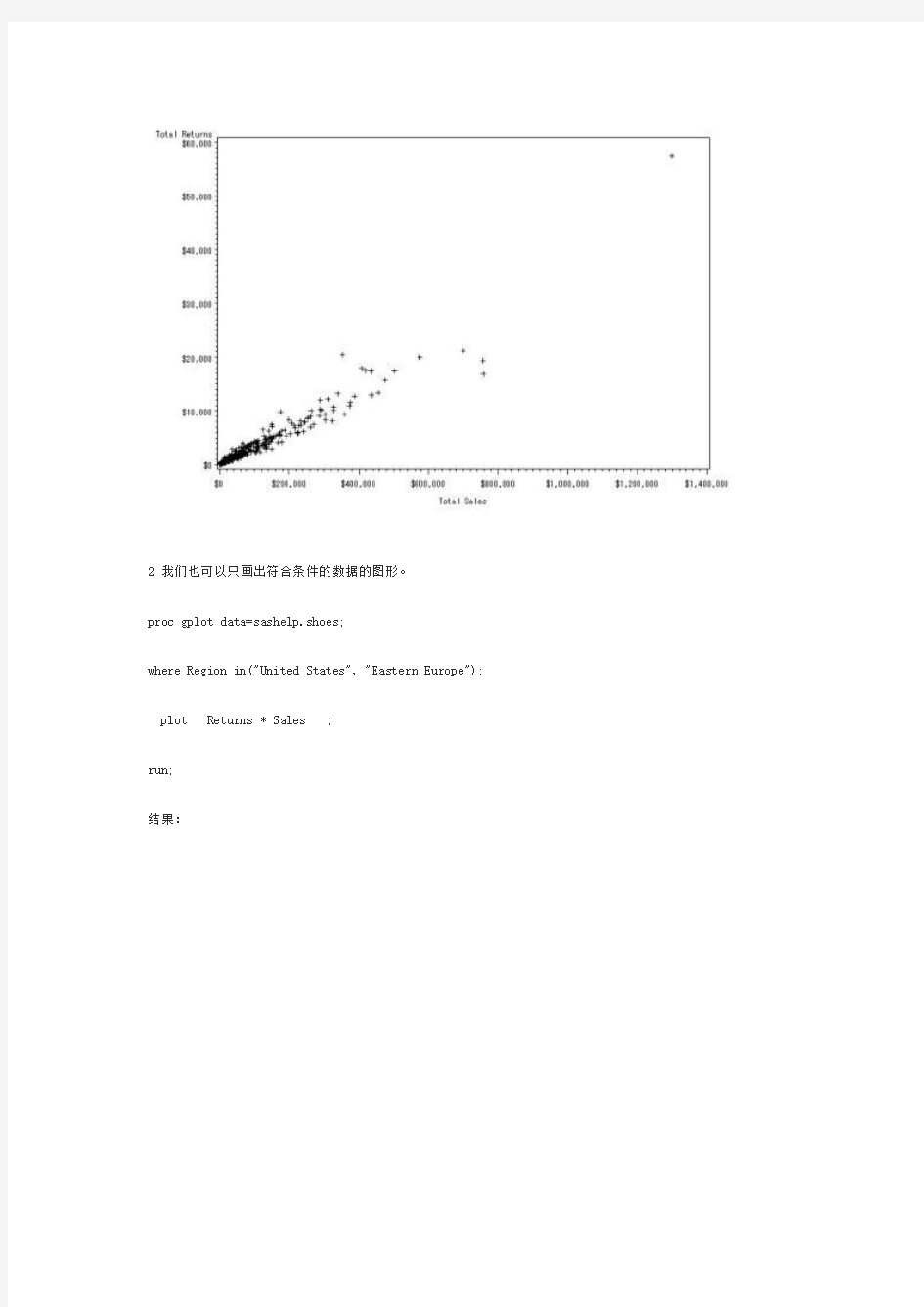
1 proc gplot的简单例子
proc gplot data=sashelp.shoes;
plot Returns * Sales ;
run;
结果:
2 我们也可以只画出符合条件的数据的图形。
proc gplot data=sashelp.shoes;
where Region in("United States", "Eastern Europe"); plot Returns * Sales ;
run;
结果:
3 输出的图像都是默认的黑色的小十字,因此我们不能区分来自不同地区的数据,下面的程序就是为了解决这一问题
proc gplot data=sashelp.shoes;
where Region in("United States", "Eastern Europe");
plot Returns * Sales= Region;
run;
结果:
这里红色的来自美国,黑色的来自东欧,当然我们也可以自己设定颜色(SAS基本颜色有:black, red, green, blue, cyan, magenta, grey, pink, orange, brown, and yellow)。
4 设定坐标轴和所有文字和颜色
proc gplot data=sashelp.shoes;
where Region in("United States", "Eastern Europe");
plot Returns * Sales= Region/
caxis=blue
ctext=red
grid;
run;
结果:
5 如果要对网格进行更精细地设置,则要用到AUTOHREF和AUTOVREF选项。AUTOHREF中,LHREF设置水平线的线类型,CHREF设置水平线的线颜色;AUTOVREF中,LVREF设置垂直线的线类型,CVREF设置垂直线的线颜色。
proc gplot data=sashelp.shoes;
where Region in("United States", "Eastern Europe");
plot Returns * Sales= Region/
autohref lhref=2
chref=lime
autovref lvref=5
cvref=pink
caxis=blue
ctext=red ;
run;
结果:
6 还可以用VAXIS和HAXIS分别设置纵轴和横轴的刻度。注意:如果某个数据超过了你指定的这个刻度,那么这个数据将不会被输出,因此在用这两个选项时要非常小心。
proc gplot data=sashelp.shoes;
where Region in("United States", "Eastern Europe");
plot Returns * Sales= Region/
vaxis=0 to 15000 by 5000
autohref lhref=2
chref=lime
autovref lvref=5
cvref=pink
caxis=blue
ctext=red ;
run;
结果:
7 下面介绍一些有关Graph相关过程的全局(global)设置
title1 c=darkblue h=2.5 f=swissb "SAS/Graph "
c=darkred h=3.0 f=swissbi "GPLOT Example"; axis1
label=(c=darkorange h=1.5 f=zapfbi
j=r "Total Returns")
offset=(0.2 in )
order=(0 to 15000 by 5000)
value=(c=darkorange f=swissl );
axis2
label=(c=darkgreen h=1.5 f=zapfbi)
order=(0 to 500000 by 50000)
value=(f=swissl c=darkgreen);
symbol1 c=red h=2 v=# ;
symbol2 c=blue h=3 v=diamond;
proc gplot data=sashelp.shoes;
where Region in("United States","Eastern Europe"); plot Returns * Sales=Region /
vaxis=axis1 haxis=axis2
autohref lhref=2 chref=lime
autovref lvref=5 cvref=pink
caxis=blue ctext=red ;
run;
结果:
我们还可以设置这些Symbol是否用线连接起来,即INTERPOLATION=(I=)设置连接方式,以及WIDTH=(W=)设置线的宽度。
symbol1 c=red h=2 v=# i=sm50s w=2;
symbol2 c=blue h=3 v=diamond i=splines w=2.5;
结果略。
8 下面开始介绍Gchart,首先是一个简单的gchart过程步的一个简单应用。
title1 c=darkblue h=2.5 f=swissb "SAS/Graph "
c=darkred h=3.0 f=swissbi "GChart Example";
proc gchart data=sashelp.shoes;
vbar3d Product /
caxis=blue
ctext=darkblue
autoref lref=2 cref=lime;
run;
结果:
9 设置背景色和图形形状
axis1
label=(c=darkgreen h=1.5 f=zapfbi)
value=(f=swissb c=darkgreen h=0.75); proc gchart data=sashelp.shoes;
vbar3d Product /
caxis=blue
ctext=darkblue
autoref lref=2 cref=lime
maxis=axis1
shape=star
cframe=cyan;
run;
10 柱状图求和显示
axis1 label=(c=darkgreen h=1.5 f=zapfbi) value=(f=swissb c=darkgreen h=0.70); axis2 label=(c=darkorange h=1.5 f=zapfbi) value=(c=darkorange f=swissl) ;
proc gchart data=sashelp.shoes;
vbar3d Product /
caxis=blue ctext=darkblue
autoref lref=2 cref=lime
sum sumvar=sales
maxis=axis1 raxis=axis2
shape=star cframe=cyan;
run;
结果:
11 用patternid将各个柱子设为不同颜色
axis1 label=(c=darkgreen h=1.5 f=zapfbi) value=(f=swissb c=darkgreen h=0.70);
axis2 label=(c=darkorange h=1.5 f=zapfbi) value=(c=darkorange f=swissl) ;
proc gchart data=sashelp.shoes;
vbar3d Product /
caxis=blue ctext=darkblue
autoref lref=2 cref=lime
sum sumvar=sales
maxis=axis1 raxis=axis2
shape=star cframe=cyan
patternid=midpoint;
run;
结果:
12 根据分组分别显示柱状图
axis1 label=(c=darkgreen h=1.5 f=zapfbi)
value=(f=swissb c=darkgreen h=0.70);
axis2 label=(c=darkorange h=1.5 f=zapfbi)
value=(c=darkorange f=swissl) ;
axis3 label=(c=blue h=1.5 f=centbi)
value=(f=swissb c=blue h=1.5);
proc gchart data=sashelp.shoes;
where Region in("United States","Western Europe"); vbar3d Product /
caxis=blue ctext=darkblue
autoref lref=2 cref=lime
sum sumvar=sales
maxis=axis1 raxis=axis2
shape=star cframe=cyan
patternid=MIDPOINT
group=Region gaxis=axis3;
run;
结果:
13 设置subgroup。
axis1 label=(c=darkgreen h=1.5 f=zapfbi)
value=(f=swissb c=darkgreen h=0.70);
axis2 label=(c=darkorange h=1.5 f=zapfbi)
value=(c=darkorange f=swissl) ;
proc gchart data=sashelp.shoes;
where Region in("United States","Western Europe"); vbar3d Product /
caxis=blue ctext=darkblue
autoref lref=2 cref=lime
sum sumvar=sales
maxis=axis1 raxis=axis2
shape=star cframe=cyan
subgroup=Region;
run;
结果:
14 下面设置legend
axis1 label=(c=darkgreen h=1.5 f=zapfbi) value=(f=swissb c=darkgreen h=0.70); axis2 label=(c=darkorange h=1.5 f=zapfbi) value=(c=darkorange f=swissl) ;
legend1 frame
position=(top center inside) label=none
value=(f=swissb h=1.5
t=1 c=red
t=2 c=green);
proc gchart data=sashelp.shoes;
where Region in("United States","Western Europe"); vbar3d Product /
caxis=blue ctext=darkblue
autoref lref=2 cref=lime
sum sumvar=sales
maxis=axis1 raxis=axis2
shape=star cframe=cyan
subgroup=Region legend=legend1;
run;
结果:
15 Goptions
太多了,就随便列一些吧:
Border|Noborder--put a border around the entire graph. Cback= -- Color of background of entire graph.
Cby= -- Color of BY line.
Ctext= -- Color for all text in the body of the graph. Ctitle= -- Color for all titles.
Device= -- Device driver.
Fby= -- Font for BY lines.
Ftext= -- Font for all text in the body of the graph. Ftitle= -- Font for all titles.
Gsfname= -- Fileref of output file.
Gsfmode=append|replace -- disposition of output file.
Hby= -- Height of BY line
Htext= -- Height of all text in the body of the graph.
Htitle= -- Height of all titles.
Reset=(all|global|axis|symbol|pattern|legend|title) -- Reset back to system default. Targetdevice= -- Device driver that will eventually be used to produce final graph. Colors=() -- Colors list.
Hsize= -- Physical size of graph in horizontal inches.
Hpos= -- Number of cells in the horizontal.
Xpixels= -- Physical size of graph in horizontal pixels.
Vsize= -- Physical size of graph in vertical inches.
Vpos= -- Number of cells in the vertical.
Ypixels= -- Physical size of graph in vertical pixels.
举例:
filename graphs 'C:\';
goptions device=gif
hpos=150 vpos=60
xpixels=1200 ypixels=800
gsfmode=replace
gsfname=graphs;
proc gchart data=sashelp.shoes;
where Region in("United States","Western Europe"); vbar3d Product /
shape=star caxis=blue ctext=black
maxis=axis1 raxis=axis2
autoref lref=2 cref=lime
cframe=cyan sum sumvar=sales
subgroup=Region patternid=subgroup
legend=legend1
name='gchart4';
run;