Jitter Analysis_The dual-Dirac

第18卷 第6期 太赫兹科学与电子信息学报Vo1.18，No.6 2020年12月 Journal of Terahertz Science and Electronic Information Technology Dec.，2020 文章编号：2095-4980(2020)06-1003-07分布式相参雷达多脉冲积累相参参数估计方法王雪琦，涂刚毅，吴少鹏(中国船舶重工集团公司第七二四研究所，江苏南京 211106)摘 要：分布式相参雷达(DCAR)是目前国内外雷达领域的重要研究方向，精确的参数估计是实现其良好相参性能的前提和核心。

基于动目标模型，提出一种基于多脉冲积累的相参参数估计方法。

该方法通过对多脉冲信号进行快、慢时间匹配滤波处理，实现多脉冲相参积累；再利用互相关法进行相参参数估计。

仿真分析对比了不同脉冲个数和不同输入信噪比下的参数估计性能和相参性能，仿真结果表明，该方法具有可行性，且可以有效提高低信噪比情况下的参数估计性能和相参性能。

关键词：分布式相参；参数估计；动目标；多脉冲积累中图分类号：TN957.51文献标志码：A doi：10.11805/TKYDA2019182Coherent parameters estimation method for distributed coherent radarbased on multi-pulse accumulationWANG Xueqi，TU Gangyi，WU Shaopeng(No.724 Research Institute of CSIC，Nanjing Jiangshu 211106，China)Abstract：Distributed Coherent Aperture Radar(DCAR) is an important research direction in the field of radar at home and abroad. Accurate parameter estimation is the premise and core of good coherenceperformance. Based on the moving target model, a coherent parameter estimation method based onmulti-pulse accumulation is proposed. The method performs fast-time and slow-time match filtering formulti-pulse signals, and obtains the results of multi-pulse coherent accumulation. Then thecross-correlation method is utilized to estimate the coherent parameters. The performance of parameterestimation and correlation under different numbers of pulses and different input signal-to-noise ratios arecompared by simulation analysis. The simulation results show that the method is feasible and caneffectively improve the performance of parameter estimation and coherence in low signal-to-noise ratio.Keywords：distributed coherence；parameter estimation；moving target；multi-pulse accumulation分布式相参雷达(DCAR)因具有较好的探测性能、高角度分辨力、灵活性和机动性等一系列技术优势而成为目前国内外雷达领域研究热点[1-5]。

the dirac-delta sequence 术语概述及解释说明1. 引言1.1 概述在数学中，Dirac-Delta序列是一种特殊的函数序列，由英国物理学家保罗·狄拉克（Paul Dirac）于20世纪提出。

Dirac-Delta序列在数学分析、信号处理和物理学等领域广泛应用，它具有独特的性质和重要的应用价值。

1.2 文章结构本文将对Dirac-Delta序列进行详细的定义、性质与应用探讨，并分析Dirac序列与Dirac-Delta序列之间的关系。

文章结构如下所示：1. 引言2. 正文3. Dirac-Delta序列的定义与性质3.1 Dirac-Delta函数的引入3.2 Dirac-Delta序列的定义3.3 Dirac-Delta序列的性质与应用4. Dirac序列与Dirac-Delta序列之间的关系4.1 Dirac序列的定义与性质4.2 Dirac序列与Dirac-Delta函数的关系5. 结论通过以上结构，读者将逐步了解Dirac-Delta序列及其相关术语，并深入探讨其定义、性质以及应用方面。

1.3 目的本文旨在向读者介绍和解释Dirac-Delta序列这一重要的数学术语及其相关概念。

通过对其定义、性质与应用的详细说明，希望读者能够更加全面地理解和掌握该序列，在实际问题中能够正确运用并深化对其的认识。

同时，本文将分析Dirac序列与Dirac-Delta序列之间的关系，从而进一步拓展读者对于这两者的认知。

在阅读本文后，读者将能够清晰了解Dirac-Delta序列，并具备一定的基础来应用该概念解决实际问题。

希望本文能够为对数学有兴趣或从事相关领域研究的人士提供帮助，并推动更多关于Dirac-Delta序列的进一步研究和应用。

2. 正文正文部分将对Dirac-Delta序列的相关概念进行详细解释和说明。

首先，我们会介绍Dirac函数的引入，然后给出Dirac-Delta序列的定义，并讨论其性质和应用。

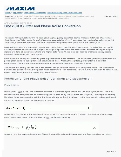
Maxim > App Notes > High-Speed Interconnect Oscillators/Delay Lines/Timers/CountersDec 10, 2004 Keywords: CLK jitter, clock jitter, phase noise, phase noise conversion, phase noise measurement, jittermeasurement, jitter and phase noise, phase noise calculation, timing errorAPPLICATION NOTE 3359Clock (CLK) Jitter and Phase Noise ConversionAbstract: This application note on clock (CLK) signal quality describes how to measure jitter and phase-noise, including period jitter, cycle-to-cycle jitter, and accumulated jitter. It describes the relationship between period jitter and phase-noise spectrum and how to convert the phase-noise spectrum to the period jitter.Clock (CLK) signals are required in almost every integrated circuit or electrical system. In today's world, digital data is processed or transmitted at higher and higher speeds, while the conversions between analog and digital signals are done at higher resolutions and higher data rates. These functions require engineers to pay special attention to the quality of clock signals.Clock quality is usually described by jitter or phase-noise measurements. The often-used jitter measurements are period jitter, cycle-to-cycle jitter, and accumulated jitter. Among these jitters, period jitter is most often encountered. Clock phase-noise measurement examines the spectrum of the clock signal.This article first briefly reviews the measurement setups for clock period jitter and phase noise. The relationship between the period jitter and the phase-noise spectrum is then described. Finally, a simple equation to convert the phase-noise spectrum to the period jitter is presented.Period Jitter and Phase Noise: Definition and MeasurementPeriod JitterPeriod jitter (J PER) is the time difference between a measured cycle period and the ideal cycle period. Due to its random nature, this jitter can be measured peak-to-peak or by root of mean square (RMS). We begin by defining the clock rising-edge crossing point at the threshold V TH as T PER(n), where n is the time domain index, as shown in Figure 1. Mathematically, we can describe J PER as:where T0 is the period of the ideal clock cycle. Since the clock frequency is constant, the random quantity J PERmust have a zero mean. Thus the RMS of J PER can be calculated by:where <•> is the expected operation. Figure 1 shows the relation between J PER and T PER in a clock waveform.Figure 1. Period jitter measurement.Phase-Noise SpectrumTo understand the definition of the phase-noise spectrum L(f), we first define the power spectrum density of a clock signal as S C(f). The S C(f) curve results when we connect the clock signal to a spectrum analyzer. The phase-noise spectrum L(f) is then defined as the attenuation in dB from the peak value of S C(f) at the clock frequency, f C, to a value of S C(f) at f. Figure 2 illustrates the definition of L(f).Figure 2. Definition of phase-noise spectrum.Mathematically, the phase-noise spectrum L(f) can be written as:Remember that L(f) presents the ratio of two spectral amplitudes at the frequencies, f C and f. The meaning of L(f) will be discussed in next section.Period Jitter (J PER) MeasurementThere are different instruments used to measure the period jitter. People most commonly use a high-precisiondigital oscilloscope to conduct the measurement. When the clock jitter is more than 5 times larger than the oscilloscope's triggering jitter, the clock jitter can be acquired by triggering at a clock rising edge and measuring it at the next rising edge. Figure 3 shows a splitter generating the trigger signal from the clock under test. This method eliminates the internal jitter from the clock source in the digital oscilloscope.Figure 3. Self-trigger jitter measurement setup.It is possible for the duration of scope trigger-delay to be longer than the period of a high-frequency clock. In that case, one must insert a delay unit in the setup that delays the first rising edge after triggering so that it can be seen on the screen.There are more accurate methods for measuring jitter. Most of these approaches use a post-sampling process of the data sampled from high-speed digital oscilloscopes to estimate the jitter according to the definitions in Equations 1 or 2. This post-sampling approach provides high-precision results, but it can only be performed with high-end digital oscilloscopes [2, 3].Phase-Noise Spectrum L(f) MeasurementAs Equation 3 showed above, L(f) can be measured with a spectrum analyzer directly from the spectrum, S C(f), of the clock signal. This approach, however, is not practical. The value of L(f) is usually larger than 100dBc which exceeds the dynamic range of most spectrum analyzers. Moreover, f C can sometimes be higher than the input-frequency limit of the analyzer. Consequently, the practical way to measure the phase noise uses a setup that eliminates the spectrum energy at f C. This approach is similar to the method of demodulating a passband signal to baseband. Figure 4 illustrates this practical setup and the signal-spectrum changes at different points in the test setup.Figure 4. Practical phase-noise measurement setup.The structure described in Figure 4 is typically called a carrier-suppress demodulator. In Figure 4, n(t) is the input to the spectrum analyzer. We will next show that by scaling down the spectrum of n(t) properly, we can obtain the dBc value of L(f).Relation between RMS Period Jitter and Phase NoiseUsing the Fourier series expansion, it can be shown that a square-wave clock signal has the same jitter behavior as its base harmonic sinusoid signal. This property makes the jitter analysis of a clock signal much easier. A sinusoid signal of a clock signal with phase noise can be written as:and the period jitter is:From Equation 4 we see that the sinusoid signal is phase modulated by the phase noise Θ(t). As the phase noise is always much smaller than π/2, Equation 4 can be approximated as:The spectrum of C(t) is then:where SΘ(f) is the spectrum of q(t). Using the definition of L(f), we can find:This illustrates that L(f) is just SΘ(f) presented in dB. This also explains the real meaning of L(f).We have now shown that the setup in Figure 4 enables the measurement of L(f). Furthermore, one can see that the signal C(t) is mixed with cos(2πf C t) and filtered by the lowpass filter. Thus, we can express the signal n(t) at the input of the spectrum analyzer as:The spectrum appears on the spectrum analyzer as:Therefore we can obtain the phase noise spectrum SΘ(f) and L(f):Then L(f) can be read in dBc directly from the spectrum of n(t) after scaled down by A²/4.From Equation 11, the mean square (MS) of Θ(t) can be calculated by:Following Equation 5 above, we finally show the relationship between the period jitter, J PER, and the phase noise spectrum, L(f), as:In some applications like SONET and 10Gb, engineers only monitor the jitter at a certain frequency band. In such acase, the RMS J PER within a certain band can be calculated by:Approximation of RMS J PER from L(f)The phase noise usually can be approximated by a linear piece-wise function when the frequency axis of L(f) is in log scale. In such a case, L(f) can be written as:where K-1 is the number of the pieces of the piece-wise function and U(f) is the step function. See Figure 5.Figure 5. A typical L(f) function.If we substitute L(f) shown in Equation 15 into Equation 14, we have:To illustrate this, the following table presents a piecewise L(f) function with f C = 155.52MHz.Table 1. Measurements of Function L(f).Frequency (Hz)101000300010000L(f) (dBc)-58-118-132-137Next we calculate the a i and b i by:The results are listed in Table 2.Table 2. Parameters to Present L(f) as a Piecewise Function.i1234f i (Hz)101000300010000a i (dBc/decade)-30-29.34-9.5N/Ab i (dBc)-58-118-132-137Substituting the Table 2 values into Equation 16, we get:The RMS jitter of the same clock measured by the setup in Figure 4 at the same band is 4.2258ps. Therefore, the proposed approximation approach for converting phase noise to jitter has proved quite accurate. In this example, the error is less than 4%.Equation 16 can also be used to estimate the required jitter limit when the phase-noise spectrum envelope is given.A simple spreadsheet file has been posted with the equation coded as an example.SummaryThis article demonstrates the exact mathematical relationship between jitter measured in time and the phase-noise measured in frequency. Many engineers concerned with signal integrity and system timing frequently question this relationship. The results presented here clearly answer the question. Based on that mathematical relationship, weproposed a method for estimating the period jitter from the phase-noise spectrum. Engineers can use this method to quickly establish a quantitative relationship between the two measurements, which will help greatly in the application or design of systems and circuits.Reference1. SEMI G80-0200, "Test Method for the Analysis of Overall Digital Timing Accuracy for Automated TestEquipment".2. Tektronix Application Note: "Understanding and Characterizing Timing Jitter"3. LeCroy White Paper: "The Accuracy of Jitter Measurements"4. David Chandler, "Phase Jitter-Phase Noise and VCXO," Corning Frequency Control Inc.Related PartsMAX9485:QuickView-- Full (PDF) Data Sheet-- Free SamplesMAX9486:QuickView-- Full (PDF) Data Sheet-- Free SamplesMAX9489:QuickView-- Full (PDF) Data SheetAutomatic UpdatesWould you like to be automatically notified when new application notes are published in your areas of interest? Sign up for EE-Mail™.Application note 3359: /an3359More InformationFor technical support: /supportFor samples: /samplesOther questions and comments: /contactAN3359, AN 3359, APP3359, Appnote3359, Appnote 3359Copyright © by Maxim Integrated ProductsAdditional legal notices: /legal。