Methods and uncertainties in bioclimatic envelope modelling under climate change

第４１卷第７期２０２１年４月生态学报ＡＣＴＡＥＣＯＬＯＧＩＣＡＳＩＮＩＣＡＶｏｌ．４１，Ｎｏ．７Ａｐｒ．，２０２１基金项目：中国科学院战略先导专项（ＸＤＡ２３０６０４０５）；国家重点研发计划（２０１６ＹＦＣ０５００６０６）；吉林省科技发展计划（２０１９０３０３０６６ＳＦ）收稿日期：２０１９⁃０８⁃２３；㊀㊀网络出版日期：２０２１⁃０１⁃２７∗通讯作者Ｃｏｒｒｅｓｐｏｎｄｉｎｇａｕｔｈｏｒ．Ｅ⁃ｍａｉｌ：ｈｕａｎｇｙｘ＠ｉｇａ．ａｃ．ｃｎＤＯＩ：１０．５８４６／ｓｔｘｂ２０１９０８２３１７５２郑伟，范高华，黄迎新，王婷，禹朴家，王鹤琪．不同密度猪毛菜形态结构性状及生物量分配策略的异速关系．生态学报，２０２１，４１（７）：２８４５⁃２８５４．ＺｈｅｎｇＷ，ＦａｎＧＨ，ＨｕａｎｇＹＸ，ＷａｎｇＴ，ＹｕＰＪ，ＷａｎｇＨＱ．ＡｌｌｏｍｅｔｒｉｃｒｅｌａｔｉｏｎｓｈｉｐｓｂｅｔｗｅｅｎｔｈｅｍｏｒｐｈｏｌｏｇｉｃａｌｔｒａｉｔｓａｎｄｂｉｏｍａｓｓａｌｌｏｃａｔｉｏｎｓｔｒａｔｅｇｉｅｓｏｆＳａｌｓｏｌａｃｏｌｌｉｎａｕｎｄｅｒｄｉｆｆｅｒｅｎｔｐｏｐｕｌａｔｉｏｎｄｅｎｓｉｔｙ．ＡｃｔａＥｃｏｌｏｇｉｃａＳｉｎｉｃａ，２０２１，４１（７）：２８４５⁃２８５４．不同密度猪毛菜形态结构性状及生物量分配策略的异速关系郑㊀伟１，范高华２，黄迎新２，∗，王㊀婷２，禹朴家２，３，王鹤琪２１吉林省教育学院，长春㊀１３００２２２中国科学院东北地理与农业生态研究所，吉林省草地畜牧重点实验室，长春㊀１３０１０２３西南大学地理科学学院，重庆金佛山喀斯特生态系统野外科学观测研究站，重庆㊀４００７１５摘要：植物的生长特性随环境条件的变化具有可塑性，而不同的环境因素对植物可塑性的影响也不尽相同㊂利用异速分析的方法，通过模拟退化草地恢复过程中猪毛菜（Ｓａｌｓｏｌａｃｏｌｌｉｎａ）的不同种群密度（１６㊁４４㊁１００㊁４００株／ｍ２），研究其形态结构性状及生物量分配策略的异速关系在种群密度间的差异㊂结果表明，种群密度增大能抑制猪毛菜的生长，而且对猪毛菜的株高㊁根长㊁一级分枝数㊁二级分枝数㊁三级分枝数以及总分枝长均产生了极显著的影响，表明种群密度的变化使得植物的高生长和侧向生长发生了显著变化㊂种群密度的变化也引起了植物生物量的变化，其中植物根㊁茎㊁叶间的生物关系是一种表观可塑性，植物的生长策略未发生改变，只是植物个体大小发生改变引起的生物量分配的变化㊂植物株高㊁总分枝长㊁一级分枝数及繁殖分配的变化，是由种群密度变化引起的，植物的适应策略发生了改变，是真正的可塑性㊂种群密度改变了植物的繁殖分配策略，而未改变植物叶的分配策略，说明当环境发生变化时，植物调整了其繁殖策略以适应环境因素的改变，以保证种群的生存繁衍㊂关键词：株高；枝条数；生物量分配；异速生长；猪毛菜ＡｌｌｏｍｅｔｒｉｃｒｅｌａｔｉｏｎｓｈｉｐｓｂｅｔｗｅｅｎｔｈｅｍｏｒｐｈｏｌｏｇｉｃａｌｔｒａｉｔｓａｎｄｂｉｏｍａｓｓａｌｌｏｃａｔｉｏｎｓｔｒａｔｅｇｉｅｓｏｆＳａｌｓｏｌａｃｏｌｌｉｎａｕｎｄｅｒｄｉｆｆｅｒｅｎｔｐｏｐｕｌａｔｉｏｎｄｅｎｓｉｔｙＺＨＥＮＧＷｅｉ１，ＦＡＮＧａｏｈｕａ２，ＨＵＡＮＧＹｉｎｇｘｉｎ２，∗，ＷＡＮＧＴｉｎｇ２，ＹＵＰｕｊｉａ２，３，ＷＡＮＧＨｅｑｉ２１ＥｄｕｃａｔｉｏｎａｌＩｎｓｔｉｔｕｔｅｏｆＪｉｌｉｎＰｒｏｖｉｎｃｅ，Ｃｈａｎｇｃｈｕｎ１３００２２，Ｃｈｉｎａ２ＮｏｒｔｈｅａｓｔＩｎｓｔｉｔｕｔｅｏｆＧｅｏｇｒａｐｈｙａｎｄＡｇｒｏｅｃｏｌｏｇｙ，ＣｈｉｎｅｓｅＡｃａｄｅｍｙｏｆＳｃｉｅｎｃｅｓ，ＪｉｌｉｎＰｒｏｖｉｎｃｉａｌＫｅｙＬａｂｏｒａｔｏｒｙｏｆＧｒａｓｓｌａｎｄＦａｒｍｉｎｇ，Ｃｈａｎｇｃｈｕｎ１３０１０２，Ｃｈｉｎａ３ＣｈｏｎｇｑｉｎｇｊｉｎｆｏＭｏｕｎｔａｉｎＦｉｅｌｄＳｃｉｅｎｔｉｆｉｃＯｂｓｅｒｖａｔｉｏｎａｎｄＲｅｓｅａｒｃｈＳｔａｔｉｏｎｆｏｒＫａｒｓｔＥｃｏｓｙｓｔｅｍ，ＳｃｈｏｏｌｏｆＧｅｏｇｒａｐｈｉｃａｌＳｃｉｅｎｃｅｓ，ＳｏｕｔｈｗｅｓｔＵｎｉｖｅｒｓｉｔｙ，Ｃｈｏｎｇｑｉｎｇ４００７１５，ＣｈｉｎａＡｂｓｔｒａｃｔ：Ｐｌａｎｔｇｒｏｗｔｈｃｈａｒａｃｔｅｒｉｓｔｉｃｓｈａｖｅｐｌａｓｔｉｃｉｔｙｉｎｒｅｓｐｏｎｓｅｔｏｃｈａｎｇｅｓｏｆｅｎｖｉｒｏｎｍｅｎｔａｌｃｏｎｄｉｔｉｏｎｓ，ａｎｄｄｉｆｆｅｒｅｎｔｅｎｖｉｒｏｎｍｅｎｔａｌｆａｃｔｏｒｓｈａｖｅｄｉｆｆｅｒｅｎｔｅｆｆｅｃｔｓｏｎｐｌａｎｔｐｌａｓｔｉｃｉｔｙ．Ｔｈｅａｌｌｏｍｅｔｒｉｃｍｅｔｈｏｄｗａｓｕｓｅｄｔｏａｎａｌｙｚｅｔｈｅｍｏｒｐｈｏｌｏｇｉｃａｌ－ｓｔｒｕｃｔｕｒａｌｔｒａｉｔｓａｎｄｂｉｏｍａｓｓａｌｌｏｃａｔｉｏｎｓｔｒａｔｅｇｉｅｓｂｙｓｉｍｕｌａｔｉｎｇｐｏｐｕｌａｔｉｏｎｄｅｎｓｉｔｉｅｓｏｆＳ．ｃｏｌｌｉｎａ（１６，４４，１００ａｎｄ４００ｐｌａｎｔｓ／ｍ２）ｄｕｒｉｎｇｔｈｅｒｅｓｔｏｒａｔｉｏｎｏｆｄｅｇｒａｄｅｄｇｒａｓｓｌａｎｄ．ＴｈｅｒｅｓｕｌｔｓｓｈｏｗｅｄｔｈａｔｔｈｅｉｎｃｒｅａｓｅｄｐｏｐｕｌａｔｉｏｎｄｅｎｓｉｔｙｃｏｕｌｄｉｎｈｉｂｉｔｔｈｅｇｒｏｗｔｈｏｆＳ．ｃｏｌｌｉｎａ．ｐｏｐｕｌａｔｉｏｎｄｅｎｓｉｔｙｈａｄｓｉｇｎｉｆｉｃａｎｔｅｆｆｅｃｔｓｏｎｐｌａｎｔｈｅｉｇｈｔ，ｒｏｏｔｌｅｎｇｔｈ，ｐｒｉｍａｒｙｂｒａｎｃｈｎｕｍｂｅｒ，ｓｅｃｏｎｄ－ｌｅｖｅｌｂｒａｎｃｈｎｕｍｂｅｒ，ｔｈｉｒｄ－ｌｅｖｅｌｂｒａｎｃｈｎｕｍｂｅｒ，ａｎｄｔｏｔａｌｂｒａｎｃｈｌｅｎｇｔｈ，ｉｎｄｉｃａｔｉｎｇｔｈａｔｐｏｐｕｌａｔｉｏｎｄｅｎｓｉｔｙｃｈａｎｇｅｓｈａｖｅｃａｕｓｅｄｓｉｇｎｉｆｉｃａｎｔｃｈａｎｇｅｓｉｎｖｅｒｔｉｃａｌａｎｄｌａｔｅｒａｌｇｒｏｗｔｈｏｆＳ．ｃｏｌｌｉｎａ．Ｐｏｐｕｌａｔｉｏｎｄｅｎｓｉｔｙｃｈａｎｇｅｓａｌｓｏ６４８２㊀生㊀态㊀学㊀报㊀㊀㊀４１卷㊀ｉｎｆｌｕｅｎｃｅｄｏｎｔｈｅｂｉｏｍａｓｓｏｆｐｌａｎｔ．Ｔｈｅｂｉｏｌｏｇｉｃａｌｒｅｌａｔｉｏｎｓｈｉｐｓｂｅｔｗｅｅｎｒｏｏｔｓ，ｓｔｅｍｓ，ａｎｄｌｅａｖｅｓａｒｅａｎ ａｐｐａｒｅｎｔｐｌａｓｔｉｃｉｔｙ ，ａｎｄｔｈｅｇｒｏｗｔｈｓｔｒａｔｅｇｙｈａｓｎｏｔｃｈａｎｇｅｄａｔａｌｌ，ｏｎｌｙｔｈｅｖａｒｉａｔｉｏｎｏｆｂｉｏｍａｓｓａｌｌｏｃａｔｉｏｎｗｅｒｅｃａｕｓｅｄｂｙｔｈｅｃｈａｎｇｅｏｆｉｎｄｉｖｉｄｕａｌｐｌａｎｔｓｉｚｅ．Ｃｈａｎｇｅｓｉｎｐｌａｎｔｈｅｉｇｈｔ，ｔｏｔａｌｂｒａｎｃｈｌｅｎｇｔｈ，ｐｒｉｍａｒｙｂｒａｎｃｈｎｕｍｂｅｒａｎｄｒｅｐｒｏｄｕｃｔｉｖｅｂｉｏｍａｓｓａｌｌｏｃａｔｉｏｎｗｅｒｅｓｉｇｎｉｆｉｃａｎｔｌｙｉｎｆｌｕｅｎｃｅｄｂｙｐｏｐｕｌａｔｉｏｎｄｅｎｓｉｔｙ，ｒｅｐｒｅｓｅｎｔｉｎｇ ｔｒｕｅ ｐｌａｓｔｉｃｉｔｙ．Ｔｈｅｒｅｓｕｌｔｓｓｈｏｗｅｄｔｈａｔｖａｒｉａｔｉｏｎｏｆｐｏｐｕｌａｔｉｏｎｄｅｎｓｉｔｙｃａｕｓｅｄｔｈｅｓｔｒａｔｅｇｙｃｈａｎｇｅｏｆｔｈｅｒｅｐｒｏｄｕｃｔｉｖｅａｌｌｏｃａｔｉｏｎｒａｔｈｅｒｔｈａｎｔｈｅｌｅａｆａｌｌｏｃａｔｉｏｎ，ｉｎｄｉｃａｔｉｎｇｔｈａｔｗｈｅｎｅｎｖｉｒｏｎｍｅｎｔｃｈａｎｇｅｓ，ｐｌａｎｔｗｏｕｌｄａｄｊｕｓｔｔｈｅｒｅｐｒｏｄｕｃｔｉｖｅｓｔｒａｔｅｇｙｔｏａｄａｐｔｔｏｓｕｒｒｏｕｎｄｉｎｇｅｎｖｉｒｏｎｍｅｎｔａｌｆａｃｔｏｒｓ，ｔｏｅｎｓｕｒｅｔｈｅｓｕｒｖｉｖａｌａｎｄｒｅｐｒｏｄｕｃｔｉｏｎｏｆｔｈｅｐｏｐｕｌａｔｉｏｎ．ＫｅｙＷｏｒｄｓ：ｐｌａｎｔｈｅｉｇｈｔ；ｂｒａｎｃｈｎｕｍｂｅｒ；ｂｉｏｍａｓｓａｌｌｏｃａｔｉｏｎ；ａｌｌｏｍｅｔｒｉｃｇｒｏｗｔｈ；Ｓａｌｓｏｌａｃｏｌｌｉｎａ植物的形态结构特征及生物量分配策略是植物内在的发育过程适应所在环境条件的结果，当植物向各个器官分配其捕获的资源时，除了自身的遗传发育规律外，主要取决于包括生物因素和非生物因素在内的环境因素的变化［１］㊂其中，植物响应种群密度所产生的变化一直是生态学领域中的一个重要研究内容［２］㊂针对植物响应种群密度在内的环境因素变异所产生的变化这一研究内容，生态学家提出了最优化分配理论，认为植物倾向于将资源分配到能够获取最受限制资源的器官［３］，然而这一理论也受到了挑战［４⁃５］㊂因为最优化分配理论的基础建立在植物生物量的分配是不依赖于个体大小的，但很多研究表明，在实际生长过程中，植物生物量的分配是受个体大小制约的［６⁃７］㊂因此如果只用最优化分配理论分析植物生物量分配的变化规律，则不能分辨植物形态结构性状及生物量分配的变化是由环境因素引起的，还是由个体大小原因导致的；而异速生长理论对解决这一问题具有重大意义［８⁃９］㊂应用异速生长方法分析植物性状的变化，不仅能将个体大小这一因素排除，揭示其真正的影响因素［１０⁃１１］，还能够系统地明确种群密度㊁个体大小以及植物性状之间的内在关系，进而揭示植物性状变化，尤其是生物量分配策略响应种群密度的变化规律㊂猪毛菜（Ｓａｌｓｏｌａｃｏｌｌｉｎａ）为一年生草本，在科尔沁地区主要分布在半流动㊁半固定㊁固定沙丘和一些环境较好的农田附近，是沙漠化土地恢复后期的一种植物［２，１２⁃１３］㊂在退化沙地或沙丘的演替过程中，猪毛菜的种群密度变化极为剧烈，但以往的研究主要集中在种子萌发［１４⁃１５］㊁叶片特性［１６］㊁光合生理特性［１７⁃１８］及植物多样性［１９］等方面，而有关种群密度变化对猪毛菜形态结构性状及生物量分配策略的影响研究较少，深入系统的研究这部分内容间的关系有助于了解土地恢复机理，对荒漠化的防治具有重要意义㊂为此，本研究深入探究了种群密度变化对猪毛菜形态结构特征的影响，以及不同种群密度猪毛菜生物量分配策略的异速关系，旨在为退化土地的恢复和荒漠化防治提供一定的理论基础，同时为健全荒漠化生态环境保护政策和制度，改善荒漠化生境，为恢复并留下可持续发展的 绿色银行 提供科学依据和理论参考㊂１㊀研究地区与研究方法１．１㊀研究区概况研究区位于内蒙古通辽市奈曼旗中科院奈曼沙漠化研究站内，地处科尔沁沙地中南部，地理位置１２０ʎ１９ᶄ １２１ʎ３５ᶄＥ，４２ʎ１４ᶄ ４３ʎ３２ᶄＮ（图１），平均海拔３６０ｍ，具有多种不同的沙地类型和植被类型，土壤和植被梯度变化十分明显［２，１６］㊂该区植被为温带半干旱草原植被，由于土地沙漠化严重，大部分地区半干旱草原植被为沙生植被所代替，植物种主要以沙米（Ａｇｒｉｏｐｈｙｌｌｕｍｓｑｕａｒｒｏｓｕｍ）㊁猪毛菜（Ｓａｌｓｏｌａｃｏｌｌｉｎａ）㊁大果虫实（Ｃｏｒｉｓｐｅｒｍｕｍｅｌｏｎｇａｔｅ）㊁糙隐子草（Ｃｌｅｉｓｔｏｇｅｎｅｓｓｑｕａｒｒｏｓａ）㊁尖头叶藜（Ｃｈｅｎｏｐｏｄｉｕｍａｃｕｍｉｎａｔｕｍ）㊁狗尾草（Ｓｅｔａｒｒｉａｖｉｒｉｄｉｓ）和委陵菜（Ｐｏｔｅｎｔｉｌｌａｂｉｆｕｒｃａ）等为主［２］㊂该区属温带半干旱大陆性季风气候，年均温６．３ħ，ȡ１０ħ年积温在３１６１．２ħ以上，无霜期约１５０ｄ㊂年均降水量３６５ｍｍ，其中７０％主要集中在６ ９月，年蒸发量１９３５．４ｍｍ［２］㊂土壤类型为沙质栗钙土，其表层土壤中沙粒和粉粒含量占比为７０％ ９０％，粘粒占比１０％ ２０％，土壤有机质含量为３％ ６％，沙土基质分布广泛［２］，风沙活动强烈，年均风速３．５ｍ／ｓ㊂图１㊀研究区分布示意图Ｆｉｇ．１㊀Ｄｉｓｔｒｉｂｕｔｉｏｎｏｆｔｈｅｒｅｓｅａｒｃｈａｒｅａ１．２㊀研究物种猪毛菜为一年生草本，高２０ １００ｃｍ，茎自基部分枝，枝互生，伸展，茎㊁枝为绿色，有白色或紫红色条纹，生硬短毛或近于无毛，叶片呈丝状圆柱形，伸展或微弯曲，长约２ ５ｃｍ，宽约０．５ １．５ｍｍ，生硬短毛，顶端有刺状尖，花序穗状，生枝条上部［２０］㊂１．３㊀试验设计２００８年５月初，在中科院奈曼沙漠化研究站内，选择质地均匀的沙质草地，通过人工撒播种植猪毛菜，根据沙地上猪毛菜自然种群随退化沙地恢复过程中的种群密度变化范围，对猪毛菜进行密度处理，共设置４个水平，每个处理水平４个重复，共１６个小区，按照随机区组方式排列，小区面积（３ｍˑ３ｍ）：１）１６株／ｍ２（Ｄ１，株距２５ｃｍ）；２）４４株／ｍ２（Ｄ２，株距１５ｃｍ）；３）１００株／ｍ２（Ｄ３，株距１０ｃｍ）；４）４００株／ｍ２（Ｄ４，株距５ｃｍ）［２］㊂在２叶期（大约２周左右）进行间苗，按照Ｄ１ Ｄ４密度处理定苗㊂整个生长阶段，除每３ ４周进行一次人工剔除其他杂草外，无其他人为干扰㊂于２００８年８月３１日进行破坏性取样，每个小区随机取样１０株，每种处理共计４０株㊂用清水将每株猪毛菜的根冲洗干净，以保证获取较为完整的根系，利用尺子测量植物的绝对高度和根长，并测量每个分枝长并计算总分枝长，并将每株植物分成根㊁茎㊁叶和繁殖器官（包括花和果）四部分，将植物放置于８０ħ烘箱内烘干称重，然后测得根㊁茎㊁叶㊁繁殖器官和地上部分等的生物量㊂１．４㊀数据分析采用ＳＰＳＳ１７．０软件和Ｒ软件的ＳＭＡＴＲ包进行数据分析㊂将数据经ｌｏｇ１０转换后，进行标准主轴回归，７４８２㊀７期㊀㊀㊀郑伟㊀等：不同密度猪毛菜形态结构性状及生物量分配策略的异速关系㊀分析种群密度对猪毛菜形态结构特征和生物量分配的异速关系，主要包括异速指数（斜率）㊁异速常数（截距）以及个体大小，并比较异速指数与３／４或１的差异［２１⁃２３］；其中采用经典的异速生长方程：Ｙ＝βＸα（１）进行权衡分析（其中：Ｙ是某个需要研究的器官属性值，Ｘ是植物个体大小或另一个器官属性值，α是异速指数，即斜率；β是异速常数，即Ｙ轴截距）㊂采用减小主轴回归（ｒｅｄｕｃｅｄｍａｊｏｒａｘｉｓｒｅｇｒｅｓｓｉｏｎ，ＲＭＡ）拟合经对数转换后的数据，确定异速指数：αＲＭＡ＝αＯＬＳˑｒ－１（２）（αＯＬＳ是最小二乘法得到的回归系数；ｒ是相关系数），以去除变量偏差对回归系数的影响［２４］㊂２㊀结果与分析２．１㊀猪毛菜形态结构性状随种群密度的变化趋势及异速关系猪毛菜的形态结构性状显著受种群密度的影响，其形态结构性状随种群密度的变化表现出相一致的异速关系㊂随种群密度的增加，株高㊁根长㊁一级分枝数㊁二级分枝数㊁三级分枝数及总分枝长均呈减少趋势（表１）㊂当种群密度按Ｄ１ Ｄ４增加时，株高分别减少７２％㊁８６％和１４％，根长分别减少１２％㊁１０％和１３％，一级分枝数分别减少９８％㊁４０４％和５％；二级分枝数和三级分枝数从Ｄ１密度增加到Ｄ２时，二级分枝数减少９０３％㊁三级分枝数减少１６７９％，到Ｄ３和Ｄ４密度时均为０，说明随着种群密度的增加，猪毛菜为了顺利完成生活史不再将能量分配到分枝的生长，而更可能倾向于种子的生长和成熟［２，２１，２５］；总分枝长随种群密度的增加分别减少３８７％㊁１０７７％和７８％㊂ＡＮＯＶＡ分析发现，株高㊁根长㊁一级分枝数㊁二级分枝数㊁三级分枝数及总分枝长均与种群密度间呈极显著负相关（Ｐ＜０．００１）（表１），表明种群密度的增加对猪毛菜株高㊁根长㊁分枝数及总分枝长起抑制作用㊂猪毛菜株高和总分枝长之间的异速指数在Ｄ１ Ｄ４密度时均与３／４间差异极显著（Ｐ＜０．００１）；株高和一级分枝数间的异速指数在Ｄ１和Ｄ２密度时与３／４间差异不显著（Ｐȡ０．０５），而在Ｄ３和Ｄ４密度时均与３／４间差异极显著（Ｐ＜０．０１），但在Ｄ１密度时又与１间差异不显著（Ｐ＝０．９７８）㊂表１㊀种群密度对猪毛菜形态性状的影响（平均值ʃ标准误）Ｔａｂｌｅ１㊀ＴｈｅｅｆｆｅｃｔｏｆＳ．ｃｏｌｌｉｎａｕｎｄｅｒｄｉｆｆｅｒｅｎｔｐｏｐｕｌａｔｉｏｎｄｅｎｓｉｔｉｅｓｏｎｔｈｅｍｏｒｐｈｏｌｏｇｉｃａｌｔｒａｉｔｓ（ｍｅａｎʃＳＥ）处理Ｔｒｅａｔｍｅｎｔ／（株／ｍ２）株高Ｐｌａｎｔｈｅｉｇｈｔ／ｃｍ根长Ｒｏｏｔｌｅｎｇｔｈ／ｃｍ一级分枝数Ｐｒｉｍａｒｙｂｒａｎｃｈｎｕｍｂｅｒ二级分枝数Ｓｅｃｏｎｄａｒｙｂｒａｎｃｈｎｕｍｂｅｒ三级分枝数Ｔｈｉｒｄｂｒａｎｃｈｎｕｍｂｅｒ总分枝长Ｔｏｔａｌｂｒａｎｃｈｌｅｎｇｔｈ／ｃｍ１６２４３．７２ʃ１３．２８２４７．４４ʃ１１．９３２０．９４ʃ１．０９６４．５９ʃ８．１９１４．４１ʃ３．５５１８５１．７８ʃ２０８．１４４４１４１．７５ʃ６．５６２２１．８１ʃ８．３７１０．５９ʃ０．８２６．４４ʃ２．２１０．８１ʃ０．５２３８０．５０ʃ７８．３１１００７０．９７ʃ５．１５２０１．０３ʃ８．６９２．１０ʃ０．４７００３２．３４ʃ８．４７４００７２．４１ʃ５．６８１７８．５６ʃ１２．６５２．００ʃ０．５１００１８．１９ʃ６．１２Ｆ８９．２３１∗∗∗７．６９７∗∗∗１２８．７７１∗∗∗４９．７２１∗∗∗１４．１８４∗∗∗５５．２０５∗∗∗㊀㊀种群密度间的差异显著性的检验采用Ｆ⁃检验；∗∗∗Ｐ＜０．００１同时发现，种群密度对猪毛菜株高：总分枝长和株高：一级分枝数的影响相一致㊂其中，种群密度对株高：总分枝长和株高：一级分枝数的异速指数和个体大小均产生了极显著的影响（Ｐ＜０．００１）（图２，表２），而异速常数均受种群密度的显著影响（Ｐ＜０．０５）㊂株高：总分枝长和株高：一级分枝数的异速指数均小于１（图２）㊂在Ｄ３和Ｄ４密度时二级分枝数和三级分枝数均为０，表明种群密度增加到Ｄ３密度时猪毛菜基于生活史的权衡分配策略，已不再将能量分配到分枝的生长㊂株高：二级分枝数和株高：三级分枝数在Ｄ１和Ｄ２密度时具有极显著的异速关系（Ｐ＜０．００１）（表２）㊂株高：二级分枝数和株高：三级分枝数的异速指数㊁异速常数及个体大小均受种群密度极显著的影响（Ｐ＜０．００１）（表２），且异速指数均小于１㊂２．２㊀猪毛菜生物量分配策略的异速关系在种群密度间的差异通过对猪毛菜各器官间异速生长的分析，发现根：地上和根：茎生物量间的异速指数及异速常数均不随种８４８２㊀生㊀态㊀学㊀报㊀㊀㊀４１卷㊀群密度的变化而变化，而种群密度对个体大小却产生了极显著的影响（Ｐ＜０．００１）（图３，表３）㊂根：地上和根：茎生物量间的异速指数均小于１（图３）㊂图２㊀株高与枝条间的异速关系Ｆｉｇ．２㊀Ｔｈｅａｌｌｏｍｅｔｒｉｃｒｅｌａｔｉｏｎｓｈｉｐｓｂｅｔｗｅｅｎｐｌａｎｔｈｅｉｇｈｔａｎｄｂｒａｎｃｈ图中１６株／ｍ２，Ｄ１㊁４４株／ｍ２，Ｄ２㊁１００株／ｍ２，Ｄ３和４００株／ｍ２，Ｄ４中数值为Ｒ软件ＳＭＡＴＲ包分析的密度的异速指数，并均在Ｒ软件中与１进行了检验表２㊀猪毛菜形态结构性状间的异速关系在密度间的差异Ｔａｂｌｅ２㊀ＴｈｅａｌｌｏｍｅｔｒｉｃｒｅｌａｔｉｏｎｓｈｉｐｓｏｆＳ．ｃｏｌｌｉｎａｕｎｄｅｒｄｉｆｆｅｒｅｎｔｄｅｎｓｉｔｉｅｓｏｎｔｈｅｍｏｒｐｈｏｌｏｇｉｃａｌｔｒａｉｔｓ性状Ｔｒａｉｔｓ株高／总分枝长Ｐｌａｎｔｈｅｉｇｈｔ／ｔｏｔａｌｂｒａｎｃｈｌｅｎｇｔｈ株高／一级分枝数Ｐｌａｎｔｈｅｉｇｈｔ／ｐｒｉｍａｒｙｂｒａｎｃｈｎｕｍｂｅｒ株高／二级分枝数Ｐｌａｎｔｈｅｉｇｈｔ／ｓｅｃｏｎｄａｒｙｂｒａｎｃｈｎｕｍｂｅｒ株高／三级分枝数Ｐｌａｎｔｈｅｉｇｈｔ／ｔｈｉｒｄｂｒａｎｃｈｎｕｍｂｅｒＳ１０．４３５０．９９６０．４０２（Ｒ２＝０．６４６）０．１８４（Ｒ２＝０．２３５）Ｓ２０．２７４０．６７１０．１９７（Ｒ２＝０．４１３）０．４１４（Ｒ２＝０．１１９）Ｓ３０．１７９０．４４６ Ｓ４０．２１６０．４８０Ｐ１＜０．００１＜０．００１＜０．００１＜０．００１Ｐ２０．００２０．００４＜０．００１＜０．００１Ｐ３＜０．００１＜０．００１＜０．００１＜０．００１㊀㊀Ｓ１表示１６株／ｍ２（Ｄ１）密度下的异速指数；Ｓ２表示４４株／ｍ２（Ｄ２）密度下的异速指数；Ｓ３表示１００株／ｍ２（Ｄ３）密度下的异速指数；Ｓ４表示４００株／ｍ２（Ｄ４）密度下的异速指数；Ｒ软件ＳＭＡＴＲ包分析的密度对异速指数㊁异速常数和个体大小的影响：Ｐ１表示各个密度处理间异速指数存在差异的显著水平；Ｐ２表示各个密度处理间异速常数存在差异的显著水平；Ｐ３表示个体大小在不同密度间的差异性分析结果表３㊀密度对猪毛菜各器官生物量分配的异速关系Ｔａｂｌｅ３㊀ＴｈｅａｌｌｏｍｅｔｒｉｃｒｅｌａｔｉｏｎｓｈｉｐｓｏｆＳ．ｃｏｌｌｉｎａｕｎｄｅｒｄｉｆｆｅｒｅｎｔｄｅｎｓｉｔｉｅｓｏｎｔｈｅｂｉｏｍａｓｓｄｉｓｔｒｉｂｕｔｉｏｎ性状Ｔｒａｉｔｓ根ʒ地上Ｒｏｏｔ／ｓｈｏｏｔｒａｔｉｏ根ʒ茎Ｒｏｏｔｓｔｅｍ叶ʒ地上Ｌｅａｖｅｓａｂｏｖｅｇｒｏｕｎｄ叶ʒ根Ｌｅａｖｅｓｒｏｏｔ叶ʒ茎Ｌｅａｖｅｓｓｔｅｍ茎ʒ地上Ｓｔｅｍａｂｏｖｅｇｒｏｕｎｄ繁殖ʒ地上Ｒｅｐｒｏｄｕｃｔｉｖｅａｂｏｖｅｇｒｏｕｎｄ繁殖ʒ根Ｒｅｐｒｏｄｕｃｔｉｖｅｒｏｏｔ繁殖ʒ茎Ｒｅｐｒｏｄｕｃｔｉｖｅｓｔｅｍ繁殖ʒ叶Ｒｅｐｒｏｄｕｃｔｉｖｅ／ｌｅａｖｅｓＰ１０．６４８０．２４２０．８９１０．４６３０．５２７０．０７７０．０１４０．１４９０．０６１０．６９６Ｐ２０．５８２０．１８３０．００２０．０３００．０３３０．０２３０．０１６０．２４００．０６４０．０５０Ｐ３＜０．００１＜０．００１＜０．００１＜０．００１＜０．００１＜０．００１＜０．００１＜０．００１＜０．００１＜０．００１㊀㊀Ｒ软件ＳＭＡＴＲ包分析的密度对异速指数㊁异速常数和个体大小的影响：Ｐ１表示各个密度处理间异速指数存在差异的显著水平；Ｐ２表示各个密度处理间异速常数存在差异的显著水平；Ｐ３表示个体大小在不同密度间的差异性分析结果随种群密度的变化，猪毛菜叶：地上㊁叶：根及叶：茎生物量间异速指数的差异不显著（Ｐ＞０．０５）（图４，表３），但种群密度对异速常数的影响显著（Ｐ＜０．０５），对个体大小产生了极显著的影响（Ｐ＜０．００１）㊂除叶：地上９４８２㊀７期㊀㊀㊀郑伟㊀等：不同密度猪毛菜形态结构性状及生物量分配策略的异速关系㊀图３㊀根生物量与其他器官生物量间的异速关系Ｆｉｇ．３㊀Ｔｈｅａｌｌｏｍｅｔｒｉｃｒｅｌａｔｉｏｎｓｈｉｐｓｂｅｔｗｅｅｎｒｏｏｔｂｉｏｍａｓｓａｎｄｏｔｈｅｒｏｒｇａｎｂｉｏｍａｓｓ图４㊀叶生物量与其他器官生物量间的异速关系Ｆｉｇ．４㊀Ｔｈｅａｌｌｏｍｅｔｒｉｃｒｅｌａｔｉｏｎｓｈｉｐｓｂｅｔｗｅｅｎｌｅａｖｅｓｂｉｏｍａｓｓａｎｄｏｔｈｅｒｏｒｇａｎｂｉｏｍａｓｓ０５８２㊀生㊀态㊀学㊀报㊀㊀㊀４１卷㊀生物量在Ｄ１和Ｄ２密度时的异速指数小于１外，其他密度时的异速指数均大于１（图４）；叶：根生物量的异速指数均大于１；叶：茎生物量的异速指数均小于１㊂研究发现，种群密度对猪毛菜茎：地上生物量的异速指数无显著影响（Ｐ＞０．０５）（图５，表３），而对异速常数产生了显著影响（Ｐ＜０．０５），对其个体大小的影响极显著（表３，Ｐ３＜０．００１）㊂茎：地上生物量的异速指数均大于１（图５，Ｐ１㊁Ｐ２㊁Ｐ３㊁Ｐ４均显著小于０．００１）㊂图５㊀茎生物量与地上器官生物量间的异速关系㊀Ｆｉｇ．５㊀Ｔｈｅａｌｌｏｍｅｔｒｉｃｒｅｌａｔｉｏｎｓｈｉｐｂｅｔｗｅｅｎｓｔｅｍｂｉｏｍａｓｓａｎｄａｂｏｖｅｇｒｏｕｎｄｂｉｏｍａｓｓ因猪毛菜集中于８月中下旬进行繁殖分配，对其种子进行收集并分析了繁殖生物量与其他器官生物量在种群密度间的差异，发现繁殖：地上生物量间的异速指数和异速常数均受种群密度的显著影响（Ｐ＞０．０５）（图６，表３），而繁殖：根㊁繁殖：茎及繁殖：叶生物量间的异速指数和异速常数均不随种群密度的变化而变化；种群密度对繁殖与其他器官间个体大小均产生了极显著的影响（Ｐ＜０．００１）㊂繁殖：地上和繁殖：叶生物量间的异速指数除在Ｄ１密度时的异速指数小于１外，其他密度时的异速指数均大于１（图６）；繁殖：根生物量间的异速指数均大于１；繁殖：茎生物量间的异速指数除在Ｄ３密度时大于１外，其他密度时均小于１㊂３㊀结论和讨论植物形态结构性状之间的关系一直是植物生态学领域研究的重点内容，但由于工作量上的限制，对植物株高㊁根长等形态结构性状研究较多，对一级分枝数㊁二级分枝数㊁三级分枝数以及总分枝长等性状研究相对较少［１０，２１］，而植物形态结构与性状间相互影响㊁相互制约，且很多植物的形态结构性状间具有显著的异速权衡关系㊂另外，植物所表现出来的性状是植物个体内在的基因型对外界环境适应的结果，植物的生长特性随环境条件的变化具有可塑性，而种群密度对植物可塑性的影响也不尽相同［２６⁃２８］㊂种群密度增大能抑制猪毛菜的生长，这与其他植物的研究结果一致［２６，２９⁃３０］，而且种群密度对猪毛菜的株高㊁根长㊁一级分枝数㊁二级分枝数㊁三级分枝数以及总分枝长均产生了极显著的影响，表明种群密度的变化严重影响了植物对各种资源的竞争能力，植物通过调整其形态结构性状适应环境的变化，以顺利高效的完成其生活史㊂生物体个体性状的关系在几个世纪前就引起了人们广泛关注，最早是Ｇａｌｉｌｅｏ通过对骨骼长度与直径的关系对各种生物性状进行预测，后来逐渐形成几何自相似模型［３１］，同时对植物的高度㊁生物量分配等关系进行大量的预测，并预测指数为２／３㊂后来，随着对代谢速率的关注，人们又发现生物体代谢速率和个体大小呈３／４次幂关系［３２］㊂生态学家对这两种发现进行了很多理论解释，最具有影响的就是生态代谢理论：基于植物在长期适应进化过程中，植物的结构能够获取最大的环境资源等假设，Ｗｅｓｔ等人提出了生态代谢理论 通过对植物导管组织的结构进行模拟，最后揭示植物代谢速率和个体大小呈３／４次幂关系，并预测植物高度㊁生物量及生物量分配的异速指数，这在生态学界引起了广泛讨论㊂近年来，有很多研究学者对该理论的结果进行了检验［２３，３３］㊂猪毛菜株高：总分枝长和株高：一级分枝数间的异速指数和异速常数均受种群密度的显著影响，表明种群密度的变化的确影响了猪毛菜株高㊁总分枝长以及一级分枝数的生长变化；说明株高和总分枝长以及株高和一级分枝数间的生长变化属于真正可塑性，随着密度变化，植物生长策略发生改变［２，１０，２１］㊂３／４是生态代谢理论的重要的一个数值，生态代谢理论预测了很多性状间的异速指数接近于这个值，因此探讨异速指数与３／４接近与否对探索生态代谢理论的适用性具有重要意义［３３］㊂１５８２㊀７期㊀㊀㊀郑伟㊀等：不同密度猪毛菜形态结构性状及生物量分配策略的异速关系㊀图６㊀繁殖器官生物量与其他器官生物量间的异速关系Ｆｉｇ．６㊀Ｔｈｅａｌｌｏｍｅｔｒｉｃｒｅｌａｔｉｏｎｓｈｉｐｓｂｅｔｗｅｅｎｒｅｐｒｏｄｕｃｔｉｖｅｂｉｏｍａｓｓａｎｄｏｔｈｅｒｏｒｇａｎｂｉｏｍａｓｓ研究发现，根：地上和根：茎生物量间的异速指数及异速常数均不随种群密度的变化而变化，而种群密度对根㊁茎以及地上生物量的大小却产生了极显著的影响，说明根和地上以及根和茎生物量间的变化是受个体大小制约的，并不受猪毛菜种群密度的变化而变化，属于表观可塑性［２，１０］㊂这表明种群密度的变化并未对根的生长产生明显影响㊂分析发现，猪毛菜根生物量和地上部分生物量间的异速指数在Ｄ１ Ｄ４密度时均接近于３／４（Ｐ＝０．１４８，Ｐ＝０．９７２，Ｐ＝０．５５４，Ｐ＝０．８２１），表明根生物量与总生物量间呈３／４次幂关系，符合生态代谢理论㊂这说明环境变化对猪毛菜根与个体大小间的异速生长不会产生影响㊂根生物量和茎生物量间的异速指数在Ｄ４密度时与３／４间差异极显著（Ｐ＜０．０１），而在Ｄ１ Ｄ３密度时与３／４间差异不显著（Ｐ＝０．５３６，Ｐ＝０．３０６，Ｐ＝０．５６１），符合生态代谢理论的预测㊂叶的性状变化反映了植物对光资源的获取能力变化情况，在本研究中，叶：地上㊁叶：根和叶：茎生物量间异速指数的差异均不显著，说明叶和地上㊁叶和根以及叶和茎生物量间的变化亦是受个体大小制约的，而不是真正响应种群密度所发生的变化，属于表观可塑性［２，１０］㊂这表明种群密度的变化亦未对叶的生长产生明显的影响［３４］㊂异速分析发现，猪毛菜叶和地上部分及叶和根生物量间的异速指数在Ｄ１ Ｄ４密度时均与３／４间差异显著（Ｐ＜０．０５），不符合生态代谢理论；叶和茎生物量间的异速指数在Ｄ１－Ｄ４密度时均与３／４间差异不显著（Ｐ＞０．０５），符合生态代谢理论；但叶生物量和地上部分生物量间的异速指数与１间差异均不显著（Ｐ＞２５８２㊀生㊀态㊀学㊀报㊀㊀㊀４１卷㊀０．０５）；而叶生物量和根生物量间的异速指数在Ｄ２和Ｄ４密度时与１间差异显著（Ｐ＜０．０５），在Ｄ１和Ｄ３密度时却均与１间差异不显著（Ｐ＝０．７３８，Ｐ＝０．１５４）㊂茎：地上生物量间异速指数的差异不显著，亦属于表观可塑性㊂茎生物量和地上部分生物量间的异速指数在Ｄ３密度时与１间差异不显著（Ｐ＝０．２１０），但在Ｄ１㊁Ｄ２和Ｄ４密度时均与１之间差异显著（Ｐ＜０．０５）㊂繁殖能力是评估种群适应环境的重要指标，本研究中种群密度对猪毛菜繁殖生物量和地上部分生物量间的异速指数和异速常数均产生了显著影响，这属于真正可塑性［１０］，说明种群密度的变化的确对其繁殖部分的生长产生了影响［３５⁃３８］㊂分析同时发现，繁殖：根㊁繁殖：茎及繁殖：叶生物量间的异速指数和异速常数均不随种群密度的变化而变化，这表明繁殖和根㊁繁殖和茎以及繁殖和叶生物量间的变化是受猪毛菜个体大小制约的，属于表观可塑性㊂繁殖生物量和地上部分生物量间的异速指数在Ｄ３密度时与１间差异显著（Ｐ＜０．０５），但在Ｄ１㊁Ｄ２和Ｄ４密度时均与１之间差异不显著（Ｐ＝０．１７２，Ｐ＝０．１８８，Ｐ＝０．１８１）；而繁殖生物量和根生物量间的异速指数在Ｄ１密度时与１间差异不显著（Ｐ＝０．７５９），但在Ｄ２ Ｄ４密度时均与１之间差异显著（Ｐ＜０．０１）；繁殖生物量和茎生物量间的异速指数在Ｄ１和Ｄ４密度时与３／４间差异不显著（Ｐ＝０．７８５，Ｐ＝０．８６３），符合生态代谢理论，在Ｄ２ Ｄ４密度时与１之间差异不显著（Ｐ＞０．０５）；繁殖生物量和叶生物量间的异速指数在Ｄ１ Ｄ４密度时与１间差异均不显著（Ｐ＞０．０５）㊂研究结果表明，种群密度的变化，促使植物的形态结构发生了显著变化，种群密度显著影响了高度与总分枝长度㊁一级分枝数等性状的异速关系，这表明，种群密度的变化使得植物的高生长和侧向生长发生了显著变化㊂植物通过调整形态结构性状以适应不同密度的竞争环境㊂种群密度的变化也引起了植物生物量的变化，植物根㊁茎㊁叶间的生物关系是一种表观可塑性，植物的生长策略未发生改变，只是植物个体大小发生改变引起的生物量分配的变化㊂植物株高㊁总分枝长㊁一级分枝数及繁殖分配的变化，是真正由种群密度变化引起的，植物的适应策略发生了改变，是真正的可塑性㊂植物叶和繁殖分配策的变化过程表明，种群密度改变了繁殖的分配策略，而未改变植物叶的分配策略，当环境发生变化时，植物调整了其繁殖策略以适应种群密度的改变，从而使得种群能顺利完成其生活史，保证种群的生存繁衍㊂致谢：感谢黄迎新研究员㊁林晓龙博士对研究和写作的帮助㊂参考文献（Ｒｅｆｅｒｅｎｃｅｓ）：［１］㊀ＷｅｉｎｉｇＣ．Ｄｉｆｆｅｒｉｎｇｓｅｌｅｃｔｉｏｎｉｎａｌｔｅｒｎａｔｉｖｅｃｏｍｐｅｔｉｔｉｖｅｅｎｖｉｒｏｎｍｅｎｔｓ：ｓｈａｄｅ⁃ａｖｏｉｄａｎｃｅｒｅｓｐｏｎｓｅｓａｎｄｇｅｒｍｉｎａｔｉｏｎｔｉｍｉｎｇ．Ｅｖｏｌｕｔｉｏｎ，２０００，５４（１）：１２４⁃１３６．［２］㊀黄迎新．四种一年生藜科植物表型可塑性研究［Ｄ］兰州：中国科学院寒区旱区环境与工程研究所，２００９．［３］㊀ＢｌｏｏｍＡＪ，ＣｈａｐｉｎＩＩＩＦＳ，ＭｏｏｎｅｙＨＡ．Ｒｅｓｏｕｒｃｅｌｉｍｉｔａｔｉｏｎｉｎｐｌａｎｔｓ⁃ａｎｅｃｏｎｏｍｉｃａｎａｌｏｇｙ．ＡｎｎｕａｌＲｅｖｉｅｗｏｆＥｃｏｌｏｇｙａｎｄＳｙｓｔｅｍａｔｉｃｓ，１９８５，１６（１）：３６３⁃３９２．［４］㊀ＣｏｌｅｍａｎＪＳ，ＭｃＣｏｎｎａｕｇｈａｙＫＤＭ，ＡｃｋｅｒｌｙＤＤ．Ｉｎｔｅｒｐｒｅｔｉｎｇｐｈｅｎｏｔｙｐｉｃｖａｒｉａｔｉｏｎｉｎｐｌａｎｔｓ．ＴｒｅｎｄｓｉｎＥｃｏｌｏｇｙ＆Ｅｖｏｌｕｔｉｏｎ，１９９４，９（５）：１８７⁃１９１．［５］㊀ＭｃｃａｒｔｈｙＭＣ，ＥｎｑｕｉｓｔＢＪ．Ｃｏｎｓｉｓｔｅｎｃｙｂｅｔｗｅｅｎａｎａｌｌｏｍｅｔｒｉｃａｐｐｒｏａｃｈａｎｄｏｐｔｉｍａｌｐａｒｔｉｔｉｏｎｉｎｇｔｈｅｏｒｙｉｎｇｌｏｂａｌｐａｔｔｅｒｎｓｏｆｐｌａｎｔｂｉｏｍａｓｓａｌｌｏｃａｔｉｏｎ．ＦｕｎｃｔｉｏｎａｌＥｃｏｌｏｇｙ，２００７，２１（４）：７１３⁃７２０．［６］㊀ＰｉｎｏＪ，ＳａｎｓＦＸ，ＭａｓａｌｌｅｓＲＭ．Ｓｉｚｅ⁃ｄｅｐｅｎｄｅｎｔｒｅｐｒｏｄｕｃｔｉｖｅｐａｔｔｅｒｎａｎｄｓｈｏｒｔ⁃ｔｅｒｍｒｅｐｒｏｄｕｃｔｉｖｅｃｏｓｔｉｎＲｕｍｅｘｏｂｔｕｓｉｆｏｌｉｕｓＬ．ＡｃｔａＯｅｃｏｌｏｇｉｃａ，２００２，２３（５）：３２１⁃３２８．［７］㊀ＯｇａｗａＫ．Ｓｉｚｅｄｅｐｅｎｄｅｎｃｅｏｆｌｅａｆａｒｅａａｎｄｔｈｅｍａｓｓｏｆｃｏｍｐｏｎｅｎｔｏｒｇａｎｓｄｕｒｉｎｇａｃｏｕｒｓｅｏｆｓｅｌｆ⁃ｔｈｉｎｎｉｎｇｉｎａｈｉｎｏｋｉ（Ｃｈａｍａｅｃｙｐａｒｉｓｏｂｔｕｓａ）ｓｅｅｄｌｉｎｇｐｏｐｕｌａｔｉｏｎ．ＥｃｏｌｏｇｉｃａｌＲｅｓｅａｒｃｈ，２００３，１８（５）：６１１⁃６１８．［８］㊀ＮｉｋｌａｓＫＪ．Ａｐｈｙｌｅｔｉｃｐｅｒｓｐｅｃｔｉｖｅｏｎｔｈｅａｌｌｏｍｅｔｒｙｏｆｐｌａｎｔｂｉｏｍａｓｓ⁃ｐａｒｔｉｔｉｏｎｉｎｇｐａｔｔｅｒｎｓａｎｄｆｕｎｃｔｉｏｎａｌｌｙｅｑｕｉｖａｌｅｎｔｏｒｇａｎ⁃ｃａｔｅｇｏｒｉｅｓ．ＮｅｗＰｈｙｔｏｌｏｇｉｓｔ，２００６，１７１（１）：２７⁃４０．［９］㊀ＳｏｌｏｗＡＲ．Ｐｏｗｅｒｌａｗｓｗｉｔｈｏｕｔｃｏｍｐｌｅｘｉｔｙ．ＥｃｏｌｏｇｙＬｅｔｔｅｒｓ，２００５，８（４）：３６１⁃３６３．［１０］㊀ＷａｎｇＴＨ，ＺｈｏｕＤＷ，ＷａｎｇＰ，ＺｈａｎｇＨＸ，ＺｈｏｕＤＷ．Ｓｉｚｅ⁃ｄｅｐｅｎｄｅｎｔｒｅｐｒｏｄｕｃｔｉｖｅｅｆｆｏｒｔｉｎＡｍａｒａｎｔｈｕｓｒｅｔｒｏｆｌｅｘｕｓ：ｔｈｅｉｎｆｌｕｅｎｃｅｏｆｐｌａｎｔｉｎｇｄｅｎｓｉｔｙａｎｄｓｏｗｉｎｇｄａｔｅ．ＣａｎａｄｉａｎＪｏｕｒｎａｌｏｆＢｏｔａｎｙ，２００６，８４（３）：４８５⁃４９２．３５８２㊀７期㊀㊀㊀郑伟㊀等：不同密度猪毛菜形态结构性状及生物量分配策略的异速关系㊀４５８２㊀生㊀态㊀学㊀报㊀㊀㊀４１卷㊀［１１］㊀ＡｌｌｅｎＡＰ，ＰｏｃｋｍａｎＷＴ，ＲｅｓｔｒｅｐｏＣ，ＭｉｌｎｅＢＴ．Ａｌｌｏｍｅｔｒｙ，ｇｒｏｗｔｈａｎｄｐｏｐｕｌａｔｉｏｎｒｅｇｕｌａｔｉｏｎｏｆｔｈｅｄｅｓｅｒｔｓｈｒｕｂＬａｒｒｅａｔｒｉｄｅｎｔａｔａ．ＦｕｎｃｔｉｏｎａｌＥｃｏｌｏｇｙ，２００８，２２（２）：１９７⁃２０４．［１２］㊀ＬｉＦＲ，ＫａｎｇＬＦ，ＺｈａｎｇＨ，ＺｈａｏＬＹ，ＳｈｉｒａｔｏＹ，ＴａｎｉｙａｍａＩ．ＣｈａｎｇｅｓｉｎｉｎｔｅｎｓｉｔｙｏｆｗｉｎｄｅｒｏｓｉｏｎａｔｄｉｆｆｅｒｅｎｔｓｔａｇｅｓｏｆｄｅｇｒａｄａｔｉｏｎｄｅｖｅｌｏｐｍｅｎｔｉｎｇｒａｓｓｌａｎｄｓｏｆＩｎｎｅｒＭｏｎｇｏｌｉａ，Ｃｈｉｎａ．ＪｏｕｒｎａｌｏｆＡｒｉｄＥｎｖｉｒｏｎｍｅｎｔｓ，２００５，６２（４）：５６７⁃５８５．［１３］㊀ＬｉＦＲ，ＺｈａｎｇＡＳ，ＤｕａｎＳＳ，ＫａｎｇＬＦ．ＰａｔｔｅｒｎｓｏｆｒｅｐｒｏｄｕｃｔｉｖｅａｌｌｏｃａｔｉｏｎｉｎＡｒｔｅｍｉｓｉａｈａｌｏｄｅｎｄｒｏｎｉｎｈａｂｉｔｉｎｇｔｗｏｃｏｎｔｒａｓｔｉｎｇｈａｂｉｔａｔｓ．ＡｃｔａＯｅｃｏｌｏｇｉｃａ，２００５，２８（１）：５７⁃６４．［１４］㊀王刚，梁学功．沙坡头人工固沙区的种子库动态．植物学报，１９９５，３７（３）：２３１⁃２３７．［１５］㊀ＤａｖｙＡＪ．Ｃｏｍｐａｒａｔｉｖｅｐｌａｎｔｅｃｏｌｏｇｙ：ａｆｕｎｃｔｉｏｎａｌａｐｐｒｏａｃｈｔｏｃｏｍｍｏｎＢｒｉｔｉｓｈｓｐｅｃｉｅｓ：ＢｙＪ．Ｐ．Ｇｒｉｍｅ，Ｊ．Ｇ．Ｈｏｄｇｓｏｎ＆Ｒ．Ｈｕｎｔ．ＵｎｗｉｎＨｙｍａｎ，Ｌｏｎｄｏｎ．１９８８．７４２ｐｐ．ＩＳＢＮ００４５８１０２８９１．Ｐｒｉｃｅ：ʕ８５．００．ＢｉｏｌｏｇｉｃａｌＣｏｎｓｅｒｖａｔｉｏｎ，１９９０，５１（２）：１６３⁃１６６．［１６］㊀毛伟，李玉霖，赵学勇，黄迎新，罗亚勇，赵玮．３种藜科植物叶特性因子对土壤养分㊁水分及种群密度的响应．中国沙漠，２００９，２９（３）：４６８⁃４７３．［１７］㊀张景光，周海燕，王新平，李新荣，王刚．沙坡头地区一年生植物的生理生态特性研究．中国沙漠，２００２，２２（４）：３５０⁃３５３．［１８］㊀曲浩，赵哈林，周瑞莲，李瑾．沙埋对两种一年生藜科植物存活及光合生理的影响．生态学杂志，２０１５，３４（１）：７９⁃８５．［１９］㊀李新荣，张景光，刘立超，陈怀顺，石庆辉．我国干旱沙漠地区人工植被与环境演变过程中植物多样性的研究．植物生态学报，２０００，２４（３）：２５７⁃２６１．［２０］㊀中国科学院植物研究所．中国植物志．第二十五卷．第二分册，被子植物门，双子叶植物纲，藜科苋科．北京：科学出版社，１９７９．［２１］㊀黄迎新，宋彦涛，范高华，周道玮．灰绿藜形态性状与繁殖性状的异速关系．草地学报，２０１５，２３（５）：９０５⁃９１３．［２２］㊀ＦａｌｓｔｅｒＤ，ＷａｒｔｏｎＤＩ，ＷｒｉｇｈｔＩＪ．ＵｓｅｒᶄｓｇｕｉｄｅｔｏＳＭＡＴＲ：ｓｔａｎｄａｒｄｉｓｅｄｍａｊｏｒａｘｉｓｔｅｓｔｓ＆ｒｏｕｔｉｎｅｓｖｅｒｓｉｏｎ２．０，ｃｏｐｙｒｉｇｈｔ２００６．（２００６⁃０３⁃１１）．ｈｔｔｐｓ：／／ｍａｎｕａｌｚｚ．ｃｏｍ／ｄｏｃ／４１５１５１１／ｕｓｅｒ⁃ｓ⁃ｇｕｉｄｅ⁃ｔｏ⁃ｓｍａｔｒ⁃⁃ｓｔａｎｄａｒｄｉｓｅｄ⁃ｍａｊｏｒ⁃ａｘｉｓ⁃ｔｅｓｔｓ⁃ａｎｄ⁃ｒｏ．［２３］㊀ＨｕａｎｇＹＸ，ＬｅｃｈｏｗｉｃｚＭＪ，ＺｈｏｕＤＷ，ＰｒｉｃｅＣＡ．Ｅｖａｌｕａｔｉｎｇｇｅｎｅｒａｌａｌｌｏｍｅｔｒｉｃｍｏｄｅｌｓ：ｉｎｔｅｒｓｐｅｃｉｆｉｃａｎｄｉｎｔｒａｓｐｅｃｉｆｉｃｄａｔａｔｅｌｌｄｉｆｆｅｒｅｎｔｓｔｏｒｉｅｓｄｕｅｔｏｉｎｔｅｒｓｐｅｃｉｆｉｃｖａｒｉａｔｉｏｎｉｎｓｔｅｍｔｉｓｓｕｅｄｅｎｓｉｔｙａｎｄｌｅａｆｓｉｚｅ．Ｏｅｃｏｌｏｇｉａ，２０１６，１８０（３）：６７１⁃６８４．［２４］㊀ＮｉｋｌａｓＫＪ．ＰｌａｎｔＡｌｌｏｍｅｔｒｙ：ｔｈｅＳｃａｌｉｎｇｏｆｆｏｒｍａｎｄＰｒｏｃｅｓｓ．Ｃｈｉｃａｇｏ：ＵｎｉｖｅｒｓｉｔｙｏｆＣｈｉｃａｇｏＰｒｅｓｓ，１９９４．［２５］㊀范高华，黄迎新，赵学勇，神祥金．种群密度对沙米异速生长的影响．草业学报，２０１７，２６（３）：５３⁃６４．［２６］㊀黄迎新，赵学勇，张洪轩，罗亚勇，毛伟．沙米表型可塑性对土壤养分㊁水分和种群密度变化的响应．应用生态学报，２００８，１９（１２）：２５９３⁃２５９８．［２７］㊀ＭｅｅｋｉｎｓＪＦ，ＭｃＣａｒｔｈｙＢＣ．ＲｅｓｐｏｎｓｅｓｏｆｔｈｅｂｉｅｎｎｉａｌｆｏｒｅｓｔｈｅｒｂＡｌｌｉａｒｉａｐｅｔｉｏｌａｔａｔｏｖａｒｉａｔｉｏｎｉｎｐｏｐｕｌａｔｉｏｎｄｅｎｓｉｔｙ，ｎｕｔｒｉｅｎｔａｄｄｉｔｉｏｎａｎｄｌｉｇｈｔａｖａｉｌａｂｉｌｉｔｙ．ＪｏｕｒｎａｌｏｆＥｃｏｌｏｇｙ，２０００，８８（３）：４４７⁃４６３．［２８］㊀ＺｈｏｕＤＷ，ＷａｎｇＴＨ，ＶａｌｅｎｔｉｎｅＩ．Ｐｈｅｎｏｔｙｐｉｃｐｌａｓｔｉｃｉｔｙｏｆｌｉｆｅ⁃ｈｉｓｔｏｒｙｃｈａｒａｃｔｅｒｓｉｎｒｅｓｐｏｎｓｅｔｏｄｉｆｆｅｒｅｎｔｇｅｒｍｉｎａｔｉｏｎｔｉｍｉｎｇｉｎｔｗｏａｎｎｕａｌｗｅｅｄｓ．ＣａｎａｄｉａｎＪｏｕｒｎａｌｏｆＢｏｔａｎｙ，２００５，８３（１）：２８⁃３６．［２９］㊀范高华，崔桢，张金伟，黄迎新，神祥金，赵学勇．密度对尖头叶藜生物量分配格局及异速生长的影响．生态学报，２０１７，３７（１５）：５０８０⁃５０９０．［３０］㊀范高华，张金伟，黄迎新，神祥金，禹朴家，赵学勇．种群密度对大果虫实形态特征与异速生长的影响．生态学报，２０１８，３８（１１）：３９３１⁃３９４２．［３１］㊀ＧａｌｉｌｅｉＧ．ＤｉｓｃｏｒｓｉｅＤｉｍｏｓｔｒａｚｉｏｎｉＭａｔｅｍａｔｉｃｈｅ，ＩｎｔｏｒｎｏａｄｕｅＮｕｏｖｅＳｃｉｅｎｚｅ．Ｌｅｉｄａ：ＡｐｐｒｅｓｓｏｇｌｉＥｌｓｅｖｉｒｉｉ，１６３８．［３２］㊀ＰａｎｔｉｎＣ．ＰｒｏｂｌｅｍｓｏｆＲｅｌａｔｉｖｅＧｒｏｗｔｈ．Ｎａｔｕｒｅ，１９３２，１２９：７７５⁃７７７．［３３］㊀ＷｅｓｔＧＢ，ＢｒｏｗｎＪＨ，ＥｎｑｕｉｓｔＢＪ．Ａｇｅｎｅｒａｌｍｏｄｅｌｆｏｒｔｈｅｏｒｉｇｉｎｏｆａｌｌｏｍｅｔｒｉｃｓｃａｌｉｎｇｌａｗｓｉｎｂｉｏｌｏｇｙ．Ｓｃｉｅｎｃｅ，１９９７，２７６（５３０９）：１２２⁃１２６．［３４］㊀ＨｕａｎｇＹＸ，ＬｅｃｈｏｗｉｃｚＭＪ，ＰｒｉｃｅＣＡ，ＬｉＬ，ＷａｎｇＹ，ＺｈｏｕＤＷ．Ｔｈｅｕｎｄｅｒｌｙｉｎｇｂａｓｉｓｆｏｒｔｈｅｔｒａｄｅ⁃ｏｆｆｂｅｔｗｅｅｎｌｅａｆｓｉｚｅａｎｄｌｅａｆｉｎｇｉｎｔｅｎｓｉｔｙ．ＦｕｎｃｔｉｏｎａｌＥｃｏｌｏｇｙ，２０１６，３０（２）：１９９⁃２０５．［３５］㊀ＳｃｈｍｉｔｔＪ，ＷｕｌｆｆＲＤ．Ｌｉｇｈｔｓｐｅｃｔｒａｌｑｕａｌｉｔｙ，ｐｈｙｔｏｃｈｒｏｍｅａｎｄｐｌａｎｔｃｏｍｐｅｔｉｔｉｏｎ．ＴｒｅｎｄｓｉｎＥｃｏｌｏｇｙ＆Ｅｖｏｌｕｔｉｏｎ，１９９３，８（２）：４７⁃５１．［３６］㊀ＤｏｕｓｔＪＬ．Ｐｌａｎｔｒｅｐｒｏｄｕｃｔｉｖｅｓｔｒａｔｅｇｉｅｓａｎｄｒｅｓｏｕｒｃｅａｌｌｏｃａｔｉｏｎ．ＴｒｅｎｄｓｉｎＥｃｏｌｏｇｙ＆Ｅｖｏｌｕｔｉｏｎ，１９８９，４（８）：２３０⁃２３４．［３７］㊀ＯｂｅｓｏＪＲ．Ｔｈｅｃｏｓｔｓｏｆｒｅｐｒｏｄｕｃｔｉｏｎｉｎｐｌａｎｔｓ．ＮｅｗＰｈｙｔｏｌｏｇｉｓｔ，２００２，１５５（３）：３２１⁃３４８．［３８］㊀ＳｕｇｉｙａｍａＳ，ＢａｚｚａｚＦＡ．Ｓｉｚｅｄｅｐｅｎｄｅｎｃｅｏｆｒｅｐｒｏｄｕｃｔｉｖｅａｌｌｏｃａｔｉｏｎ：ｔｈｅｉｎｆｌｕｅｎｃｅｏｆｒｅｓｏｕｒｃｅａｖａｉｌａｂｉｌｉｔｙ，ｃｏｍｐｅｔｉｔｉｏｎａｎｄｇｅｎｅｔｉｃｉｄｅｎｔｉｔｙ．ＦｕｎｃｔｉｏｎａｌＥｃｏｌｏｇｙ，１９９８，１２（２）：２８０⁃２８８．。

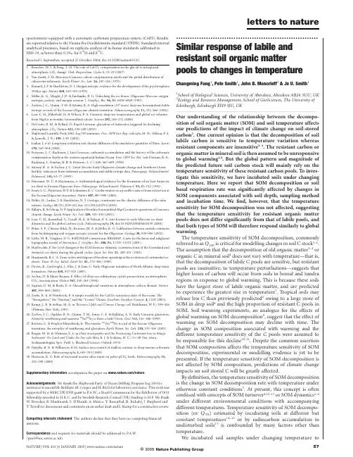
spectrometer equipped with a automatic carbonate preparation system(CAPS).Results are reported relative to the Vienna Pee Dee Belemnite standard(VPDB).Standard external analytical precision,based on replicate analysis of in-house standards calibrated to NBS-19,is better than0.1‰for d18O and d13C.Received1September;accepted25October2004;doi:10.1038/nature03135.1.Broecker,W.S.&Peng,T.-H.The role of CaCO3compensation in the glacial to interglacialatmospheric CO2change.Glob.Biogeochem.Cycles1,15–29(1987).2.Van Andel,T.H.Mesozoic/Cenozoic calcite compensation depth and the global distribution ofcalcareous sediments.Earth Planet.Sci.Lett.26,187–194(1975).3.Kennett,J.P.&Shackleton,N.J.Oxygen isotopic evidence for the development of the psychrosphere38Myr ago.Nature260,513–515(1976).ler,K.G.,Wright,J.D.&Fairbanks,R.G.Unlocking the ice house:Oligocene-Miocene oxygenisotopes,eustasy,and margin erosion.J.Geophys.Res.96,B4,6829–6849(1991).5.Zachos,J.C.,Quinn,T.M.&Salamy,K.A.High-resolution(104years)deep-sea foraminiferal stableisotope records of the Eocene-Oligocene climate transition.Palaeoceanography11,251–266(1996).6.Lear,C.H.,Elderfield,H.&Wilson,P.A.Cenozoic deep-sea temperatures and global ice volumesfrom Mg/Ca in benthic foraminiferal calcite.Science287,269–272(2000).7.DeConto,R.M.&Pollard,D.Rapid Cenozoic glaciation of Antarctica triggered by decliningatmospheric CO2.Nature421,245–249(2003).8.Shipboard Scientific Party2002.Leg199summary.Proc.ODP Init.Rep.(eds Lyle,M.W.,Wilson,P.A.&Janecek,T.R.)199,1–87(2002).skar,J.et al.Long term evolution and chaotic diffusion of the insolation quantities of Mars.Icarus170,343–364(2004).10.Peterson,L.C.Backman,te Cenozoic carbonate accumulation and the history of the carbonatecompensation depth in the western equatorial Indian Ocean.Proc.ODP Sci.Res.(eds Duncan,R.A., Backman,J.,Dunbar,R.B.&Peterson,L.C.)115,467–489(1990).11.Salamy,K.A.&Zachos,test Eocene-Early Oligocene climate change and Southern Oceanfertility:inferences from sediment accumulation and stable isotope data.Palaeogeogr.Palaeoclimatol.Palaeoecol.145,61–77(1999).12.Ehrmann,W.U.&Mackensen,A.Sedimentological evidence for the formation of an East Antarcticice sheet in Eocene/Oligocene time.Palaeogeogr.Palaeoclimatol.Palaeoecol.93,85–112(1992). 13.Ivany,L.C.,Patterson,W.P.&Lohmann,K.C.Cooler winters as a possible cause of mass extinction atthe Eocene/Oligocene boundary.Nature407,887–890(2000).14.Pa¨like,H.,Laskar,J.&Shackleton,N.J.Geologic constraints on the chaotic diffusion of the solarsystem.Geology32(11),929–932doi:10.1130/G20750(2004).15.Billups,K.&Schrag,D.P.Application of benthic foraminiferal Mg/Ca ratios to questions of Cenozoicclimate change.Earth Planet.Sci.Lett.209,181–195(2003).16.Lear,C.H.,Rosenthal,Y.,Coxall,H.K.&Wilson,te Eocene to early Miocene ice-sheetdynamics and the global carbon cycle.Paleoceanography19,doi:10.1029/2004PA001039(2004). 17.Pekar,S.F.,Christie-Blick,N.,Kominz,M.A.&Miller,K.G.Calibration between eustatic estimatesfrom backstripping and oxygen isotopic records for the Oligocene.Geology30,903–906(2002). 18.Lythe,M.B.,Vaughan,D.G.&BEDMAP Consortium,BEDMAP:A new ice thickness and subglacialtopographic model of Antarctica.J.Geophys.Res.106,B6,11335–11351(2001).19.Huybrechts,P.Sea-level changes at the LGM from ice-dynamic reconstructions of the Greenland andAntarctic ice sheets during the glacial cycles.Quat.Sci.Rev.21,203–231(2002).20.Hindmarsh,R.C.A.Time-scales and degrees of freedom operating in the evolution of continental ice-sheets.Trans.R.Soc.Edinb.Earth Sci.81,371–384(1990).21.Davies,R.,Cartwright,J.,Pike,J.&Line,C.Early Oligocene initiation of North Atlantic deep waterformation.Nature410,917–920(2001).22.Archer,D.&Maier-Reimer,E.Effect of deep-sea sedimentary calcite preservation on atmosphericCO2concentration.Nature367,260–263(1994).23.Sigman,D.M.&Boyle,E.A.Glacial/interglacial variations in atmospheric carbon dioxide.Nature407,859–869(2000).24.Zeebe,R.E.&Westbroek,P.A simple model for the CaCO3saturation state of the ocean:The“Strangelove,”the“Neritan,”and the“Cretan”Ocean.Geochem.Geophys.Geosyst.4,1104(2003).25.Kump,L.R.&Arthur,M.A.in Tectonics Uplift and Climate Change(ed.Ruddiman,W.F.)399–426(Plenum,New York,1997).26.Zachos,J.C.,Opdyke,B.N.,Quinn,T.M.,Jones,C.E.&Halliday,A.N.Early Cenozoic glaciation,Antarctic weathering and seawater87Sr/86Sr;is there a link?Chem.Geol.161,165–180(1999). 27.Ravizza,G.&Peucker-Ehrenbrink,B.The marine187Os/188Os record of the Eocene-Oligocenetransition:the interplay of weathering and glaciation.Earth Planet.Sci.Lett.210,151–165(2003).28.Berger,W.H.&Winterer,E.L.in Plate Stratigraphy and the Fluctuating Carbonate line in PelagicSediments:On Land and Under the Sea(eds Hsu¨,K.J.&Jenkyns,H.C.)11–48(Int.Assoc.Sedimentologists Spec.Publ.1,Blackwell Science,Oxford,1974).29.Opdyke,B.N.&Wilkinson,B.H.Surface area control of shallow cratonic to deep marine carbonateaccumulation.Paleoceanography3,685–703(1989).30.Harrison,K.G.Role of increased marine silica input on paleo-pCO2levels.Paleoceanography15,292–298(2000).Supplementary Information accompanies the paper on /nature. Acknowledgements We thank the Shipboard Party of Ocean Drilling Program Leg199for assistance at sea and M.Bolshaw,M.Cooper and H.Birch for laboratory assistance.This work was supported by a NERC UK ODP grant to P.A.W.,a Royal Commission for the Exhibition of1851 fellowship awarded to H.K.C.and by Swedish Research Council(VR)funding to H.P.We thank W.Broecker,R.Hindmarsh,S.D’Hondt,A.Merico,Y.Rosenthal,R.Rickaby,J.Shepherd and T.Tyrrell for discussions and comments on an earlier draft and L.Kump for a constructive review.Competing interests statement The authors declare that they have no competingfinancial interests.Correspondence and requests for materials should be addressed to P.A.W.(paw1@)............................................................... Similar response of labile and resistant soil organic matterpools to changes in temperature Changming Fang1,Pete Smith1,John B.Moncrieff2&Jo U.Smith11School of Biological Sciences,University of Aberdeen,Aberdeen AB243UU,UK 2Ecology and Resource Management,School of GeoSciences,The University of Edinburgh,Edinburgh EH93JU,UK ............................................................................................................................................................................. Our understanding of the relationship between the decompo-sition of soil organic matter(SOM)and soil temperature affects our predictions of the impact of climate change on soil-stored carbon1.One current opinion is that the decomposition of soil labile carbon is sensitive to temperature variation whereas resistant components are insensitive2–4.The resistant carbon or organic matter in mineral soil is then assumed to be unresponsive to global warming2,4.But the global pattern and magnitude of the predicted future soil carbon stock will mainly rely on the temperature sensitivity of these resistant carbon pools.To inves-tigate this sensitivity,we have incubated soils under changing temperature.Here we report that SOM decomposition or soil basal respiration rate was significantly affected by changes in SOM components associated with soil depth,sampling method and incubation time.Wefind,however,that the temperature sensitivity for SOM decomposition was not affected,suggesting that the temperature sensitivity for resistant organic matter pools does not differ significantly from that of labile pools,and that both types of SOM will therefore respond similarly to global warming.The temperature sensitivity of SOM decomposition,commonly referred to as Q10,is critical for modelling changes in soil C stock3–6. The assumption that the decomposition of old organic matter2–3or organic C in mineral soil4does not vary with temperature—that is, that the decomposition of labile C pools are sensitive,but resistant pools are insensitive,to temperature perturbations—suggests that higher losses of carbon will occur from soils in boreal and tundra regions in response to global warming.This is because these soils have the largest store of labile organic matter,and are predicted to experience the greatest rise in temperature7.Tropical soils may release less C than previously predicted4owing to a large store of SOM in deep soil8and the high proportion of resistant C pools in SOM.Soil warming experiments,an analogue for the effects of global warming on SOM decomposition9,suggest that the effect of warming on SOM decomposition may decline with time.The change in SOM composition associated with warming and the different temperature sensitivity of the C pools were assumed to be responsible for this decline10–11.Despite the common assertion that SOM composition affects the temperature sensitivity of SOM decomposition,experimental or modelling evidence is yet to be presented.If the temperature sensitivity of SOM decomposition is not affected by SOM composition,predictions of climate change impacts on soil stored C will be greatly affected.By definition,the temperature sensitivity of SOM decomposition is the change in SOM decomposition rate with temperature under otherwise constant conditions5.At present,this concept is often confused with concepts of SOM turnover4,12–13or SOM dynamics2–4 under different environmental conditions with accompanying different temperatures.Temperature sensitivity of SOM decompo-sition(or Q10)estimated by incubating soils at different but constant temperatures14–16or by radiocarbon accumulation in undisturbed soils13is confounded by many factors other than temperature.We incubated soil samples under changing temperature toletters to natureNATURE|VOL433|6JANUARY2005|/nature57©2005Nature Publishing Groupinvestigate the influence of SOM composition on the temperature dependence of SOM decomposition.Figure 1shows that soil C contents for both labile components (water-dissolved organic carbon (DOC),microbial carbon (C mic )and K 2SO 4-extracted carbon (C KSO ))and the total organic carbon (TOC),are signifi-cantly lower in the subsoil (20–30cm)than in the surface soil (0–10cm).The ratio of DOC:TOC and C KSO :TOC declined signifi-cantly with soil depth (F ¼28.5and 36.1,respectively,P ,0.0001),but C mic :TOC was not significantly affected by depth (F ¼1.9,P ,0.2).After the initial flush of CO 2emission,soil basal respi-ration rate at 208C was (mean ^s.e.m.)6.67^0.46m g CO 2per g dry soil per h for root-free samples in the 0–10cm layer,but only 1.92^0.20m g CO 2per g dry soil per h for the 20–30cm layer.Corresponding values were 6.27^0.66and 1.47^0.16for intact samples.Over a period up to 88days,the subsoil respired only ,0.29^0.13of the CO 2respired in the surface soil.These results indicate that soil basal respiration rate is closely related to variations in C pools occurring at different soil depths.Q 10values for individual soil samples varied in the range 1.97–2.21during the early stage of incubation (up to day 10).No significant correlation was found between Q 10and the rate of basal respiration.Relationships in Fig.1between respiration rate,Q 10value and SOM pools reflect the long-term acclimation of the microbial community to the environment (such as temperature,moisture and O 2)associated with soil depths.During the incubation,there was a significant decline in the labile components (Fig.2c,d,f).After 108days incubation,DOC was 0.73^0.14and C KSO was 0.62^0.065of initial values when averaged over all samples.The greatest variation following incu-bation was observed in C mic .The average C mic at day 42was only 0.43^0.13of the initial content,and less than 0.10^0.0057after 108days incubation.Changes in the average TOC during incu-bation were not significant (Fig.2b).At the end of the incubation,average TOC was 0.94^0.19of the initial content.Soil respiration rate consistently declined with time (Fig.2e).The association between respiration rate and C mic during the incubation suggests that the variation in microbial biomass may be a major cause of the temporal changes in soil respiration.The response of soil basal respiration to temperature was notaffected by the depletion of labile C during the incubation.Q 10values averaged for all samples were in the range 2.01–2.30for the whole incubation period (Fig.2a).There is no significant change in Q 10for soil basal respiration with incubation time,despite the fact that Q 10was more variable during the later stages of incubation.As time progressed,the resistant C component contributed a greater portion of the total soil basal respiration owing to the depletion of labile C pools (Supplementary Fig.2).The Q 10value for soil basal respiration should gradually decrease if resistant C is significantly different from labile pools and insensitive to temperature variation (Supplementary Fig.3).A constant Q 10for soil basal respiration suggests that the temperature dependence of resistant C is not significantly different from that for labile pools.In most incubation experiments,soil samples have been sepa-rately incubated at different but constant temperatures 12,14,15.Three different methods have been used to estimate SOM decomposition and its temperature sensitivity:the total mass loss 3,17,the time required for a given percentage of mass loss 17,and the soil respir-ation rate 14,18.A decline in soil respiration rate was commonly observed as incubation times increased 14,17,19,20.This decline is expected to be greater at higher than at lower temperatures because of the greater depletion and degradation of C pools 21.Temperature sensitivity is likely to be underestimated if turnover rate is derived from studies of total mass loss for a given time period or from respiration rates at different constant temperatures,owing to the higher decline in C turnover rate at higher temperature.If Q 10is estimated using the time required for a given percentage of mass loss,the value will be overestimated.In this case,temporal effects on estimated C turnover rate are more pronounced at lower temperatures than at higher temperatures.Data of total mass loss from soil incubations longer than one year were used to support the opinion that decomposition rates of organic matter in mineral soil do not vary with temperature 4.Estimated C turnover rates from a long-term incubation will be significantly different from those occurring in the field,owing to the quick decline in soil microbial biomass and respiration rate during incubation.In such exper-iments,the temperature sensitivity of SOM decomposition may have been seriously biased or underestimated because respiration rates at all temperatures are close to zero at the later stage of incubation.In soil warming experiments,the observed decline of warming effects on SOM decomposition with time 11does not necessarily mean that the decomposition of resistant C is less sensitive to elevated temperature than the labile component.Provided that the increase in net primary production (NPP)due to warming islessFigure 1Soil carbon components,respiration rate and associated Q 10values with respect to soil depth and sampling method (four replicates for each sample).Respiration rate was an average of data measured at 208C in days 3and 5.The Q 10value was estimated with soil respiration rates under changing temperature for the period of days 3–10.All values are normalized against that of surface root-free sample.Soil respiration rate is significantly related to concentrations of C pools owing to soil depth andsampling method,but Q 10does not change with respiration rate or C concentrations.Error bars indicate standard deviation.DOC,dissolved organic carbon;TOC,total organiccarbon.Figure 2Variations in respiration rate and soil carbon pools with increasing incubation time.Values are averages of all four samples,and normalized by initial values.a ,Q 10value;b ,TOC;c ,DOC;d ,K 2SO 4-extracted C;e ,respiration rate at 208C;and f ,microbial biomass C.Error bars are standard deviation.Respiration rate declined rapidly owing to the depletion of labile components (DOC,C KSO and C mic ),but the Q 10value of soil respiration remained unchanged.letters to natureNATURE |VOL 433|6JANUARY 2005|/nature58© 2005Nature Publishing Groupthan the increase in SOM decomposition rate,a decline in warming effect on SOM decomposition is always expected.In the long-term, the microbial community may become acclimated to warming with changed activities.The contribution of this acclimation is not yet clear.For long-term climate change,the response of the resistant pool of SOM plays a critical role in regulating soil C stocks.Given the predicted climate change in Europe in the next century,the greatest loss of SOM is expected in soils where the present mean annual temperature(MAT)is less than48C,and this net release of SOM will gradually decrease with MAT gradient(Fig.3a–c).(This predicted climate change is climate forcing according to the implementation by the Hadley Centre Climate Model(HadCM3) of the Intergovernmental Panel on Climate Change(IPCC)A1FI (world market–fossil fuel intensive)emission scenario22.)With a moderate change in the temperature sensitivity of the resistant C pool(humus pool of the Rothamsted Carbon Model23only),from Q10¼2.98to about2.58(at108C),sensitivity induced change will significantly reduce the net SOM release in temperate soils(present MAT.48C).By2100,the reduction in SOM loss could be up to 46%in arable soil,37%in grassland,and32%in forest for regions where the present MAT is greater than158C(Fig.3d).At the global scale,this reduction will be large enough to change our prediction of the magnitude and spatial pattern of SOM stocks in the future.Our study does not support the opinion that resistant C pools are significantly less responsive to temperature variation than labile C pools.A MethodsSoil samples(intact and root-free)were collected from a middle-aged plantation of Sitka spruce(Picea sitchensis)in Scotland(568370N,38480W).Mineral soils were collected from four locations in the site at depths of0–10,20–30cm.Root-free samples were made by sieving soil through a2mm mesh to remove plant detritus,root and gravel.For each depth,approximately600–800g soil was taken and packed into a chamber to the original bulk density.Intact soil samples(,10£10cm)were taken next to each root-free sample, following the method of ref.5.Soil samples were analysed to determine TOC24,DOC25and C KSO26.C mic was determined by fumigation extraction26.Samples(16in total)were incubated in the laboratory using a programmable water bath(developed in The University of Edinburgh,UK).Temperature was changed commonly between4and448C (continuously increased from the lowest to the highest with a step of48C and then decreased,reaching a new temperature within two hours).Each temperature was held for about9h.Before and after each round of temperature change,soils were kept at208C for a few days.Soil moisture contents were monitored and adjusted accordingly by adding water at the surface of the soil sample,and fresh air was continuously passed through each chamber during the incubation.Respired CO2was measured with an infrared gas analyser in differential mode,logged every second for7min for each chamber,but only the average over the last four minutes was used.The16chambers were measured sequentially,and four rounds of measurement were made before changing to another temperature.During each round of temperature change,the mean respiration rate at a given temperature was an average of values measured at that temperature when the temperature was increasing and decreasing(Supplementary Fig.1).Mean respiration rates at different temperatures werefitted with an exponential model5ðR¼a exp½ln Q10ðT=10Þ Þto calculate the Q10 value.More information about data analysis is included in the Supplementary Methods, which also explain how we assessed contributions of the resistant C pool to the total SOM decomposition and its Q10.Received30July;accepted22October2004;doi:10.1038/nature03138.1.Lenton,T.M.&Huntingford,C.Global terrestrial carbon storage and uncertainties in its temperaturesensitivity examined with a simple model.Glob.Change Biol.9,1333–1352(2003).2.Liski,J.,Ilvesniemi,H.,Ma¨kela¨,A.&Westman,C.J.CO2emissions from soil in response to climaticwarming are overestimated—The decomposition of old soil organic matter is tolerant of temperature.Ambio28,171–174(1999).3.Thornley,J.H.M.&Cannell,M.G.R.Soil carbon storage response to temperature:a hypothesis.Ann.Bot.87,591–598(2001).4.Giardina,C.P.&Ryan,M.G.Evidence that decomposition rates of organic carbon in mineral soil donot vary with temperature.Nature404,858–861(2000).5.Fang,C.&Moncrieff,J.B.The dependence of soil CO2efflux on temperature.Soil Biol.Biochem.33,155–165(2001).6.Sanderman,J.,Amundson,R.G.&Baldocchi,D.D.Application of eddy covariance measurements tothe temperature dependence of soil organic matter mean residence time.Glob.Biogeochem.Cycles17, doi:10.1029/2001GB001833(2003).7.Schlesinger,W.H.&Andrews,J.A.Soil respiration and the global carbon cycle.Biogeochemistry48,7–20(2000).8.Jobba´gy,E.G.&Jackson,R.B.The vertical distribution of soil organic carbon and its relation toclimate and vegetation.Ecol.Appl.10,423–436(2000).9.Rustad,L.E.et al.A meta-analysis of the response of soil respiration,net nitrogen mineralization,andaboveground plant growth to experimental ecosystem warming.Oecologia126,543–562(2001). 10.Peterjohn,W.T.,Melillo,J.M.&Bowles,S.T.Soil warming and trace gasfluxes:experimental designand preliminaryflux results.Oecologia93,18–24(1993).11.Peterjohn,W.T.et al.Response of trace gasfluxes and N availability to experimentally elevated soiltemperature.Ecol.Appl.4,617–625(1994).12.Dalias,P.,Anderson,J.M.,Bottner,P.&Couˆteaux,M.-M.T emperature responses of carbonmineralization in conifer forest soils from different regional climates incubated under standard laboratory conditions.Glob.Change Biol.6,181–192(2001).13.Trumbore,S.E.,Chadwick,O.A.&Amundson,R.Rapid exchange between soil carbon andatmospheric carbon dioxide driven by temperature change.Science272,393–396(1996).14.Winkler,J.P.,Cherry,R.S.&Schlesinger,W.H.The Q10relationship of microbial respiration in atemperate forest soil.Soil Biol.Biochem.28,1067–1072(1996).15.MacDonald,N.W.,Zak,D.R.&Pregitzer,K.S.Temperature effects on kinetics of microbialrespiration and net nitrogen and sulfur mineralization.Soil Sci.Soc.Am.J.59,233–240(1995). 16.Ross,D.J.&Tate,K.R.Microbial C and N,and respiratory activity,in litter and soil of a southernbeech(Nothofagus)forest:distribution and properties.Soil Biol.Biochem.25,477–483(1994). 17.Reichstein,M.,Bednorz,F.,Broll,G.&Ka¨tterer,T.T emperature dependence of carbon mineralisation:conclusions from a long-term incubation of subalpine soil samples.Soil Biol.Biochem.32,947–958 (2000).18.Fierer,N.,Allen,A.S.,Schimel,J.P.&Holden,P.A.Controls on microbial CO2production:acomparison of surface and subsurface soil horizon.Glob.Change Biol.9,1322–1332(2003).19.Lovell,R.D.&Jarvis,S.C.Soil microbial biomass and activity in soil from different grasslandmanagement treatments stored under controlled conditions.Soil Biol.Biochem.30,2077–2085 (1998).20.Lomander,A.,Ka¨tterer,T.&Andre´n,O.Carbon dioxide evolution from top-and subsoil as affected bymoisture and constant andfluctuating temperature.Soil Biol.Biochem.30,2017–2022(1998). 21.Grisi,B.,Grace,C.,Brookes,P.C.,Benedetti,A.&Dell’abate,M.T.Temperature effects on organicmatter and microbial biomass dynamics in temperate and tropical soils.Soil Biol.Biochem.30, 1309–1315(1998).22.IPCC.Special Report on Emissions Scenarios(Cambridge Univ.Press,Cambridge,UK,2000).23.Coleman,K.&Jenkinson,D.S.in Evaluation of Soil Organic Matter Models Using Existing Long-TermDatasets(eds Powlson,D.S.,Smith,P.&Smith,J.U.)237–246(NATO ASI Series I Vol.38,Springer, Heidelberg,1996).24.Allen,S.E.,Grimshaw,H.M.,Parkingson,J.A.&Quarmby,C.Chemical Analysis of EcologicalMaterials137–139(Blackwell Scientific,Oxford,1974).25.Martin-Olmedo,P.&Rees,R.M.Short-term N availability in response to dissolved organic-carbonfrom poultry manure,alone or in combination with cellulose.Biol.Fert.Soils29,386–393(1999).26.O¨hlinger,R.in Methods in Soil Biology(eds Schinner,F.et al.)56–58(Springer,Berlin,1995). Supplementary Information accompanies the paper on /nature. Acknowledgements We thank M.Wattenbarch and C.Zhang for assistance with the modelling. The pan-European modelling used data sets arising from the EU-funded ATEAM project. Competing interests statement The authors declare that they have no competingfinancial interests.Correspondence and requests for materials should be addressed to C.F.(c.fang@).Figure3Changes in soil C by2100for European soils.The baseline(solid lines in a–c)was from the original Roth-C model23projection(Q10¼2.98at108C for all C pools).Thetemperature sensitivity of humus was changed to80%of the original value(Q10¼2.58at108C,dashed lines in a–c).The loss of soil C is an average of all grid cells(21,976cellsat100£100resolution)according to present MAT.The percentage of net soil C loss withmodified Q10¼2.58for humus is relative to baseline decreases with MAT gradient(d).SOM,soil organic matter.letters to natureNATURE|VOL433|6JANUARY2005|/nature59©2005Nature Publishing Group。

IPCC第五次评估报告不确定性处理方法的介绍孙颖;秦大河;刘洪滨【摘要】由于自然气候系统极端复杂,具有内在混沌的特性,并包括各种时间尺度的非线性反馈,因此,气候变化无论观测,还是预估都存在不确定性.一些不确定性可用某些数值范围来表述,而另一些不确定性则可表述为专家对某些科学发现认识的信度.每一种不确定性的评估都需要专家进行判断,后一种不确定性更是如此[1].【期刊名称】《气候变化研究进展》【年(卷),期】2012(008)002【总页数】4页(P150-153)【作者】孙颖;秦大河;刘洪滨【作者单位】中国气象局国家气候中心,北京100081;中国气象局,北京100081;中国气象局国家气候中心,北京100081【正文语种】中文由于自然气候系统极端复杂，具有内在混沌的特性，并包括各种时间尺度的非线性反馈，因此，气候变化无论观测，还是预估都存在不确定性。

一些不确定性可用某些数值范围来表述，而另一些不确定性则可表述为专家对某些科学发现认识的信度。

每一种不确定性的评估都需要专家进行判断，后一种不确定性更是如此[1]。

在科学评估中，决策者需要的不仅仅是对所感兴趣的数值（如全球平均地表温度变化）范围的表述，而且还需要科学家给出这种定量陈述可靠性的基本信息。

政府间气候变化专门委员会（IPCC）的气候变化科学评估从一开始就认识到表述不确定性的重要性。

在第一次评估报告中，IPCC明确地把对事件的科学认识分为确定的、能够可信地计算得出的、预测的、基于作者判断的等几类，这些分类如今看来仍然非常重要。

IPCC第二次评估报告指出，需要用客观、一致的方法来确定和描述气候变化科学的信度水平。

在确定信度水平时，确保作者们所使用的信息可以追溯到有关的科学文献，从而有效地满足对客观性的要求。

IPCC第三次评估报告是第一个试图针对不同学科和广泛的国际读者群来描述不确定性的科学评估报告，“可能性”和“信度”语言的使用成为第三次评估报告的一个特征。

nature climate change的气候科学文章Nature is a scientific journal that covers all topics in nature, from天文学 to环境科学. Here are some climate change-related articles that have been published in Nature: 1. "NASA证据表明全球变暖在阿尔卑斯山脉中形成" (2021, p.38) - This article discusses a study that found that a shift in the Earth"s axis over the past century has led to a rise in global temperatures that has affected the snowpack in the mountains of阿尔卑斯山脉.2. "气候变化对南极洲冰盖的影响:一份全球变化的证据" (2020, p. 4) - This article discusses a study that found that the melting of the polar ice caps has led to a decline in the冰盖厚度 and increase in the area of sea level rise in南极洲.3. "全球变暖对生物多样性的影响:新的证据和挑战" (2020, p.11) - This article discusses a study that found that the global warming has led to a decline in biodiversity and the loss of important habitats, such as forests and ecosystems, that support life.4. "气候变化如何影响海洋生态系统:一个全球变化的例子" (2020, p. 10) - This article discusses a study that found that the warming of the Earth"s surface is driving changes in the 海洋生态系统, such as the decline of珊瑚礁 and the rise of尺紀梁海, that can impact global trade and coastal security.5. "气候变化如何影响农业和生态系统服务:来自中国的证据" (2020, p. 19) - This article discusses a study that found that the warming has led to a decline in agricultural productivity and the loss of important生态系统服务, such as game species and birdlife, that support human well-being.These articles provide a great overview of the latest research on climate change and its impact on nature.。

平衡态和瞬变气候对人类活动强迫的响应张明华【摘要】海陆气耦合模式，是用来定量描述过去气候变化的成因和预报未来气候变化的唯一数学工具。

由于大气反馈过程的差异，特别是云辐射反馈的差异，这些模式对外强迫的平衡态响应有相当大的差异。

然而，参加政府间气候变化专门委员会(Inter-governmental Panel on Climate Change，IPCC)第4次评估报告(Assessment Report，AR4)的所有耦合模式，对20世纪气候的模拟结果均非常相似。

本文研究了这种相似性的产生原因及启示。

结果表明，若大气反馈越大，则气候对外强迫的响应时滞越长、与深海的热交换越多、模式中海洋涌升流的影响越大。

这3种同样重要的物理机制共同作用，降低了瞬变气候变化对模式差异的敏感性；然而，在较长的时间尺度上，模式间大气反馈过程差异将在多个方面显现出来。

【期刊名称】《大气科学学报》【年(卷),期】2011(034)003【总页数】12页(P257-268)【关键词】平衡态气候响应；瞬变气候响应；人类活动强迫；大气反馈过程【作者】张明华【作者单位】美国纽约州立大学石溪分校，海洋和大气科学学院，美国纽约，11794【正文语种】中文【中图分类】P4350 引言气候敏感度是指全球平均表面温度对某种特定外强迫的响应程度。

人类燃烧化石燃料导致了大气中的温室气体不断增加。

认知全球表面温度对人类活动响应的程度，即气候系统的敏感度，是近30 a的研究热点之一(Randall et al.，2007)。

耦合模式(Coupled General Circulation Models，CGCMs)是研究气候敏感度的少数几个有效工具之一。

早期研究采用的是带有海洋混合层的大气环流模式。

在定常外强迫条件下，人们通过积分模式到平衡态去研究气候敏感度(Hansen et al.，1984;Wetherald and Manabe，1988)。

DOI: 10.1126/science.1220854, 773 (2013);339 Science et al.Marc André Meyers ConnectionsStructural Biological Materials: Critical Mechanics-MaterialsThis copy is for your personal, non-commercial use only.clicking here.colleagues, clients, or customers by , you can order high-quality copies for your If you wish to distribute this article to othershere.following the guidelines can be obtained by Permission to republish or repurpose articles or portions of articles): May 1, 2013 (this information is current as of The following resources related to this article are available online at/content/339/6121/773.full.html version of this article at:including high-resolution figures, can be found in the online Updated information and services, /content/339/6121/773.full.html#ref-list-1, 12 of which can be accessed free:cites 51 articles This article/cgi/collection/mat_sci Materials Sciencesubject collections:This article appears in the following registered trademark of AAAS.is a Science 2013 by the American Association for the Advancement of Science; all rights reserved. The title Copyright American Association for the Advancement of Science, 1200 New York Avenue NW, Washington, DC 20005. (print ISSN 0036-8075; online ISSN 1095-9203) is published weekly, except the last week in December, by the Science o n M a y 1, 2013w w w .s c i e n c e m a g .o r g D o w n l o a d e d f r o mStructural BiologicalMaterials:CriticalMechanics-Materials ConnectionsMarc AndréMeyers,1,2*Joanna McKittrick,1Po-Yu Chen3Spider silk is extraordinarily strong,mollusk shells and bone are tough,and porcupine quills and feathers resist buckling.How are these notable properties achieved?The building blocks of the materials listed above are primarily minerals and biopolymers,mostly in combination;the first weak in tension and the second weak in compression.The intricate and ingenious hierarchical structures are responsible for the outstanding performance of each material.Toughness is conferred by the presence of controlled interfacial features(friction,hydrogen bonds,chain straightening and stretching);buckling resistance can be achieved by filling a slender column with a lightweight foam.Here,we present and interpret selected examples of these and other biological materials.Structural bio-inspired materials design makes use of the biological structures by inserting synthetic materials and processes that augment the structures’capability while retaining their essential features.In this Review,we explain this idea through some unusual concepts.M aterials science is a vibrant field of in-tellectual endeavor and research.Thisfield applies physics and chemistry, melding them in the process,to the interrela-tionship between structure,properties,and perform-ance of complex materials with technological applications.Thus,materials science extends these rigorous scientific disciplines into complex ma-terials that have structures providing properties and synergies beyond those of pure and simple solids.Initially geared at synthetic materials,ma-terials science has recently extended its reach into biology,especially into the extracellular matrix, whose mechanical properties are of utmost im-portance in living organisms.Some of the semi-nal work and important contributions in this field are either presented or reviewed in(1–5).There are a number of interrelated features that define biological materials and distinguish them from their synthetic counterparts[inspired by Arzt(6)]: (i)Self-assembly.In contrast to many synthetic processes to produce materials,the structures are assembled from the bottom up,rather than from the top down.(ii)Multi-functionality.Many com-ponents serve more than one purpose.For exam-ple,feathers provide flight capability,camouflage, and insulation,whereas bones provide structural framework,promote the growth of red blood cells, and provide protection to the internal organs.(iii) Hierarchy.Different,organized scale levels(nano-to ultrascale)confer distinct and translatable prop-erties from one level to the next.We are starting to develop a systematic and quantitative understandingof this hierarchy by distinguishing the character-istic levels,developing constitutive descriptionsof each level,and linking them through appro-priate and physically based equations,enabling afull predictive understanding.(iv)Hydration.Theproperties are highly dependent on the level ofwater in the structure.There are some exceptions,such as enamel,but this rule applies to mostbiological materials and is of importance to me-chanical properties such as strength(which isdecreased by hydration)and toughness(which isincreased).(v)Mild synthesis conditions.Themajority of biological materials are fabricated atambient temperature and pressure as well as in anaqueous environment,a notable difference fromsynthetic materials fabrication.(vi)Evolution andenvironmental constraints.The limited availabil-ity of useful elements dictates the morphologyand resultant properties.The structures are notnecessarily optimized for all properties but arethe result of an evolutionary process leading tosatisfactory and robust solutions.(vii)Self-healingcapability.Whereas synthetic materials undergodamage and failure in an irreversible manner,biological materials often have the capability,due to the vascularity and cells embedded in thestructure,to reverse the effects of damage byhealing.The seven characteristics listed above arepresent in a vast number of structures.Nevertheless,the structures of biological materials can bedivided into two broad classes:(i)non-mineralized(“soft”)structures,which are composed of fibrousconstituents(collagen,keratin,elastin,chitin,lignin,and other biopolymers)that display widelyvarying mechanical properties and anisotropiesdepending on the function,and(ii)mineralized(“hard”)structures,consisting of hierarchicallyassembled composites of minerals(mainly,butnot solely,hydroxyapatite,calcium carbonate,and amorphous silica)and organic fibrous com-ponents(primarily collagen and chitin).The mechanical behavior of biological con-stituents and composites is quite diverse.Bio-minerals exhibit linear elastic stress-strain plots,whereas the biopolymer constituents are non-linear,demonstrating either a J shape or a curvewith an inflection point.Foams are characterizedby a compressive response containing a plastic orcrushing plateau in which the porosity is elim-inated.Many biological materials are compositeswith many components that are hierarchicallystructured and can have a broad variety of con-stitutive responses.Below,we present some of thestructures and functionalities of biological ma-terials with examples from current research.Here,we focus on three points:(i)How high tensilestrength is achieved(biopolymers),(ii)how hightoughness is attained(composite structures),and(iii)how bending resistance is achieved in light-weight structures(shells with an interior foam).Structures in Tension:Importance of BiopolymersThe ability to sustain tensile forces requires aspecific set of molecular and configurational con-formations.The initial work performed on exten-sion should be small,to reduce energy expenditure,whereas the material should stiffen close to thebreaking point,to resist failure.Thus,biopolymers,such as collagen and viscid(catching spiral)spidersilk,have a J-shaped stress-strain curve where mo-lecular uncoiling and unkinking occur with con-siderable deformation under low stress.This stiffening as the chains unfurl,straighten,stretch,and slide past each other can be repre-sented analytically in one,two,and three dimen-sions.Examples are constitutive equations initiallydeveloped for polymers by Ogden(7)and Arrudaand Boyce(8).An equation specifically proposedfor tissues is given by Fung(3).A simpler for-mulation is given here;the slope of the stress-strain(s-e)curve increases monotonically with strain.Thus,one considers two regimes:(i)unfurlingand straightening of polymer chainsd sd eºe nðn>1Þð1Þand(ii)stretching of the polymer chain backbonesd sd eºEð2Þwhere E is the elastic modulus of the chains.Thecombined equation,after integrating Eqs.1and2,iss=k1e n+1+H(e c)E(e–e c)(3)Here k1is a parameter,and H is the Heavisidefunction,which activates the second term at e=e c,where e c is a characteristic strain at whichcollagen fibers are fully extended.Subsequent straingradually becomes dominated by chain stretch-ing.The computational results by Gautieri et al.(9)on collagen fibrils corroborate Eq.3for n=1.This corresponds to a quadratic relation between1Department of Mechanical and Aerospace Engineering andMaterials Science and Engineering Program,University ofCalifornia,San Diego,La Jolla,CA92093,USA.2Department ofNanoengineering,University of California,San Diego,La Jolla,CA92093,USA.3Department of Materials Science and En-gineering,National Tsing Hua University,Hsinchu30013,Taiwan,Republic of China.*To whom correspondence should be addressed.E-mail:mameyers@ SCIENCE VOL33915FEBRUARY2013773o n M a y 1 , 2 0 1 3 w w w . s c i e n c e m a g . o r g D o w n l o a d e d f r o mstress and strain (s ºe 2),which has the char-acteristic J shape.Collagen is the most important structural bio-logical polymer,as it is the key component in many tissues (tendon,ligaments,skin,and bone),as well as in the extracellular matrix.The de-formation process is intimately connected to the different hierarchical levels,starting with the poly-peptides (0.5-nm diameter)to the tropocollagen molecules (1.5-nm diameter),then to the fibrils (~40-to 100-nm diameter),and finally to fibers (~1-to 10-m m diameter)and fascicles (>10-m m diameter).Molecular dynamics computations (9)of entire fibrils show the J -curve response;these computational predictions are well matched to atomic force microscopy (AFM)(10),small-angle x-ray scattering (SAXS)(11),and experiments by Fratzl et al .(12),as shown in Fig.1A.The effect of hydration is also seen and is of great impor-tance.The calculated density of collagen de-creases from 1.34to 1.19g/cm 3with hydration and is accompanied by a decrease in the Young ’s modulus from 3.26to 0.6GPa.The response of silk and spider thread is fascinating.As one of the toughest known ma-terials,silk also has high tensile strength and extensibility.It is composed of b sheet (10to 15volume %)nanocrystals [which consist of highly conserved poly-(Gly-Ala)and poly-Ala domains]embedded in a disordered matrix (13).Figure 1B shows the J -shape stress-strain curve and molecular configurations for the crystalline domains in silkworm (Bombyx mori )silk (14).Similar to collagen,the low-stress region corre-sponds to uncoiling and straightening of the pro-tein strands.This region is followed by entropic unfolding of the amorphous strands and then stiffening due to load transfer to the crystalline b sheets.Despite the high strength,the major mo-lecular interactions in the b sheets are weak hy-drogen bonds.Molecular dynamics simulations,Fig.1.Tensile stress-strain relationships in bio-polymers.(A )J -shaped curve for hydrated and dry collagen fibrils obtained from molecular dynamics (MD)simulations and AFM and SAXS studies.At low stress levels,considerable stretching occurs due to the uncrimping and unfolding of molecules;at higher stress levels,the polymer backbone stretches.Adapted from (9,12).(B )Stretching of dragline spider silk and molecular schematic of the protein fibroin.At low stress levels,entropic effects domi-nate (straightening of amorphous strands);at higher levels,the crystalline parts sustain the load.(C )Mo-lecular dynamics simulation of silk:(i)short stack and (ii)long stack of b -sheet crystals,showing that a higher pullout force is required in the short stack;for the long stack,bending stresses become im-portant.Hydrogen bonds connect b -sheet crystals.Adapted from (14).(D )Egg whelk case (bioelastomer)showing three regions:straightening of the a helices,the a helix –to –b sheet transformation,and b -sheet extension.A molecular schematic is shown.Adapted from (18).300.000.2Yield pointEntropic unfoldingMD simulationsStick slipStiffening β-crystal123456700012345670102030405050010001500200025050075010001250150017500.40.60.80.010.020.030.040.05MD wet (Gautieri et al)SAXS (Sasaki and Odajima)AFM (Aladin et al)MD dry (Gautieri et al)2520151050S t r e s s (M P a )S t r e s s(M P a )StrainABCDStrain (m/m)Length (nm)Length (nm)Stick-slip deformation (robust)"brittle" fracture (fragile)i iiP u l l -o u t f o r c e (p N )00.20.4Native state Unloading: reformation of α-helicesDomain 4: Extension andalignmentof β-sheets0.60.8ε=0ε4ε=01.0012345StrainS t r e s s (M P a )E n e r g y /v o l u m e (k c a l /m o l /n m 3)L e n g t hI I II II III IIIIVIVFDomain 3: Formation of β-sheetsfrom random coilsε3Domain 2: Extension of random coilsε2Domain 1: Unraveling of α-helicesinto random coilsε1Toughness (MD)Resilience (MD)T=-1°C T=20°C T=40°C T=60°C T=80°C15FEBRUARY 2013VOL 339SCIENCE 774REVIEWo n M a y 1, 2013w w w .s c i e n c e m a g .o r g D o w n l o a d e d f r o mshown in Fig.1C,illustrate an energy dissipative stick-slip shearing of the hydrogen bonds during failure of the b sheets (14).For a stack with a height L ≤3nm (left-hand side of Fig.1C),the shear stresses are more substantial than the flex-ure stresses,and the hydrogen bonds contribute to the high strength obtained (1.5GPa).How-ever,if the stack of b sheets is too high (right-hand side of Fig.1C),it undergoes bending with tensile separation between adjacent sheets.The nanoscale dimension of the b sheets allows for a ductile instead of brittle failure,resulting in high toughness values of silk.Thus,size affects the mechanical response considerably,changing the deformation characteristics of the weak hydro-gen bonds.This has also been demonstrated in bone (15–17),where sacrificial hydrogen bonds between mineralized collagen fibrils contribute to the excellent fracture resistance.Other biological soft materials have more complex responses,marked by discontinuities in d s /d e .This is the case for wool,whelk eggs,silks,and spider webs.Several mechanisms are responsible for this change in slope;for instance,the transition from a -to b -keratin,entropic changes with strain (such as those prevalent in rubber,where chain stretching and alignment decrease entropy),and others.The example of egg whelk is shown in Fig.1D (18).In this case,there is a specific stress at which a -keratin heli-ces transform to b sheets,with an associated change in length.Upon unloading,the reverse occurs,and the total reversible strain is,therefore,extensive.This stress-induced phase transforma-tion is similar to what occurs in shape-memory alloys.Thus,this material can experience sub-stantial reversible deformation (up to 80%)in a reversible fashion,when the stress is raised from 2to 5MPa,ensuring the survival of whelk eggs,which are continually swept by waves.These examples demonstrate the distinct properties of biopolymers that allow these ma-terials to be strong and highly extensible with distinctive molecular deformation characteristics.However,many interesting biological materials are composites of flexible biopolymers and stiff minerals.The combination of these two constit-uents leads to the creation of a tough material.Imparting Toughness:Importance of Interfaces One hallmark property of most biological com-posites is that they are tough.Toughness is defined as the amount of energy a material ab-sorbs before it fails,expressed asU ¼∫e fs d eð4Þwhere U is the energy per volume absorbed,s is the stress,e is the strain,and e f is the failure strain.Tough materials show considerable plastic deformation (or permanent damage)coupled with considerable strength.This maximizes the integral expression in Eq.4.Biological com-posite materials (for example,crystalline and noncrystalline components)have a plethora oftoughening mechanisms,many of which depend on the presence of interfaces.As a crack im-pinges on an interface or discontinuity in the material,the crack can be deflected around the interface (requiring more energy to propagate than a straight crack)or can drive through it.The strength of biopolymer fibers in tension im-pedes crack opening;bridges between micro-cracks are another mechanism.The toughening mechanisms have been divided into intrinsic (ex-isting in the material ahead of crack)and extrinsic (generated during the progression of failure)cat-egories (19).Thus,toughening is accomplished by a wide variety of stratagems.We illustrate this concept for four biological materials,shown in Fig.2.All inorganic materials contain flaws and cracks,which reduce the strength from the theo-retical value (~E /10to E /30).The maximum stress (s max )a material can sustain when a preexisting crack of length a is present is given by the Griffith equations max ¼ffiffiffiffiffiffiffiffiffiffi2g s E p a r ¼YK Icffiffiffiffiffip ap ð5Þwhere E is the Young ’s modulus,g s is the sur-face (or damage)energy,and Y is a geometric parameter.K Ic ¼Y −1ffiffiffiffiffiffiffiffiffiffi2g s E p is the fracture toughness,a materials property that expresses the ability to resist crack propagation.Abalone (Haliotis rufescens )nacre has a fracture tough-ness that is vastly superior to that of its major constituent,monolithic calcium carbonate,due to an ordered assembly consisting of mineral tiles with an approximate thickness of 0.5m m and a diameter of ~10m m (Fig.2A).Additionally,this material contains organic mesolayers (separated by ~300m m)that are thought to be seasonal growth bands.The tiles are connected by mineral bridges with ~50-nm diameter and are separated by organic layers,consisting of a chitin network and acidic proteins,which,when combined,have a similar thickness to the mineral bridge diame-ters.The Griffith fracture criterion (Eq.5)can be applied to predict the flaw size (a cr )at which the theoretical strength s th is achieved.With typical values for the fracture toughness (K Ic ),s th ,and E ,the critical flaw size is in the range of tens of nanometers.This led Gao et al .(20)to propose that at sufficiently small dimensions (less than the critical flaw size),materials become insensitive to flaws,and the theoretical strength (~E /30)should be achieved at the nanoscale.However,the strength of the material will be determined by fracture mechanisms operating at all hierar-chical levels.The central micrograph in Fig.2A shows how failure occurs by tile pullout.The interdigitated structure deflects cracks around the tiles instead of through them,thereby increasing the total length of the crack and the energy needed to fracture (increasing the toughness).Thus,we must de-termine how effectively the tiles resist pullout.Three contributions have been identified and are believed to operate synergistically (21).First,themineral bridges are thought to approach thetheoretical strength (10GPa),thereby strongly attaching the tiles together (22).Second,the tile surfaces have asperities that are produced during growth (23)and could produce frictional resist-ance and strain hardening (24).Third,energy is required for viscoelastic deformation (stretching and shearing)of the organic layer (25).One important aspect on the mechanical prop-erties is the effect of alignment of the mineral crystals.The oriented tiles in nacre result in an-isotropic properties with the strength and modulus higher in the longitudinal (parallel to the organic layers)than in the transverse direction.For a composite with a dispersed mineral m of volume fraction V m embedded in a biopolymer (bp)matrix that has a much lower strength and Young ’s modulus than the mineral,the ratio of the lon-gitudinal (L)and transverse (T)properties P (such as elastic modulus)can be expressed,in simpli-fied form,asP L P T ¼P mP bpV m ð1−V m Þð6ÞThus,the longitudinal properties are much higher than the transverse properties.This aniso-tropic response is also observed in other oriented mineralized materials,such as bone and teeth.Another tough biological material is the exo-skeleton of an arthropod.In the case of marine animals [for instance,lobsters (26,27)and crabs (28)],the exoskeleton structure consists of layers of mineralized chitin in a Bouligand arrange-ment (successive layers at the same angle to each other,resulting in a helicoidal stacking sequence and in-plane isotropy).These layers can be en-visaged as being stitched together with ductile tubules that also perform other functions,such as fluid transport and moisture regulation.The cross-ply Bouligand arrangement is effective in crack stopping;the crack cannot follow a straight path,thereby increasing the materials ’toughness.Upon being stressed,the mineral components frac-ture,but the chitin fibers can absorb the strain.Thus,the fractured region does not undergo physical separation with dispersal of fragments,and self-healing can take place (29).Figure 2B shows the structure of the lobster (Homarus americanus )exoskeleton with the Bouligand ar-rangement of the fibers.Bone is another example of a biological ma-terial that demonstrates high toughness.Skeletal mammalian bone is a composite of hydroxyapatite-type minerals,collagen and water.On a volu-metric basis,bone consists of ~33to 43volume %minerals,32to 44volume %organics,and 15to 25volume %water.The Young ’s modulus and strength increase,but the toughness decreases with increasing mineral volume fraction (30).Cortical (dense)mammalian bone has blood ves-sels extending along the long axis of the limbs.In animals larger than rats,the vessel is encased in a circumferentially laminated structure called the osteon.Primary osteons are surrounded by hypermineralized regions,whereas secondary SCIENCEVOL 33915FEBRUARY 2013775REVIEWo n M a y 1, 2013w w w .s c i e n c e m a g .o r g D o w n l o a d e d f r o m(remodeled)osteons are surrounded by a cement line (also of high mineral content)(31).In mam-malian cortical bone,the following intrinsic toughening mechanisms have been identified:molecular uncoiling and intermolecular sliding of collagen,fibrillar sliding of collagen bonds,and microcracking of the mineral matrix (19).Extrinsic mechanisms are collagen fibril bridging,uncracked ligament bridging,and crack deflec-tion and twisting (19).Rarely does a limb bone snap in two with smooth fracture surfaces;the crack is often deflected orthogonal to the crack front direction.In the case of (rehydrated)elk (Cervus elaphus )antler bone (shown in Fig.2C)(32),which has the highest toughness of any bone type by far (33),the hypermineralized re-gions around the primary osteons lead to crackdeflection,and the high amount of collagen (~60volume %)adds mechanisms of crack re-tardation and creates crack bridges behind the crack front.The toughening effect in antlers has been estimated as:crack deflection,60%;un-cracked ligament bridges,35%;and collagen as well as fibril bridging,5%(33).A particu-larly important feature in bone is that the fracture toughness increases as the crack propagates,as shown in the plot.This plot demonstrates the crack extension resistance curve,or R -curve,behavior,which is the rate of the total energy dissipated as a function of the crack size.This occurs by the activation of the extrinsic tough-ening mechanisms.In this manner,it becomes gradually more difficult to advance the crack.In human bone,the cracks are deflected and/ortwisted around the cement lines surrounding the secondary osteons and also demonstrate R -curve behavior (34).The final example illustrating how the presence of interfaces is used to retard crack propagation is the glass sea sponge (Euplectella aspergillum ).The entire structure of the V enus ’flower basket is shown in Fig.2D.Biological silica is amorphous and,within the spicules,consists of concentric layers,separated by an organic material,silicatein (35,36).The flexure strength of the spicule notably exceeds (by approximately fivefold)that of monolithic glass (37).The principal reason is the presence of interfaces,which can arrest and/or deflect the crack.Biological materials use ingenious meth-ods to retard the progression of cracks,therebyAbalone shell: NacreMineral bridgesLobsterDeer antlerChitin fibril networkHuman cortical boneMineral crystallitesPrimary osteonsSubvelvet/compact Subvelvet/cCompact Comp p actTransition zoneCancellousCollagen fibrilsDeep sea spongeSkeletonSpicules20 mm1 cmHuman cortical boneElk antlerTransverseIn-plane longitudinalASTM validASTM invalid Mesolayers ABCD0.1 mm500 nm500 nm ˜1 nm˜3 nm˜20 nmCrack extension, ⌬a (mm)T o u g h n e s s , J (k J m -2)50 nm200 nm 10 ␮m500 nm2 ␮m1 ␮m200 ␮m300 ␮m˜10 ␮m0.010.11101000.20.40.6500 00 nm50 nmFig.2.Hierarchical structures of tough biological materials demonstrating the heterogeneous interfaces that provide crack deflection.(A )Abalone nacre showing growth layers (mesolayers),mineral bridges between mineral tiles and asperities on the surface,the fibrous chitin network that forms the backbone of the inorganic layer,and an example of crack tortuosity in which the crack must travel around the tiles instead of through them [adapted from (4,21)].(B )Lobster exoskeleton showing the twisted plywood structure of the chitin (next to the shell)and the tubules that extend from the chitin layers to the animal [adapted from (27)].(C )Antler bone image showing the hard outer sheath (cortical bone)surrounding the porous bone.The collagen fibrils are highly aligned in the growth direction,with nanocrystalline minerals dispersed in and around them.The osteonal structure in a cross section of cortical bone illustrates the boundaries where cracks perpendicular to the osteons can be directed [adapted from (33)].ASTM,American Society for Testing and Mate-rials.(D )Silica sponge and the intricate scaffold of spicules.Each spicule is a circumferentially layered rod:The interfaces between the layers assist in ar-resting crack anic silicate in bridging adjacent silica layers is observed at higher magnification (red arrow)(36).15FEBRUARY 2013VOL 339SCIENCE776REVIEWo n M a y 1, 2013w w w .s c i e n c e m a g .o r g D o w n l o a d e d f r o mincreasing toughness.These methods operate at levels ranging from the nanoscale to the structur-al scale and involve interfaces to deflect cracks,bridging by ductile phases (e.g.,collagen or chitin),microcracks forming ahead of the crack,delocal-ization of damage,and others.Lightweight Structures Resistant to Bending,Torsion,and Buckling —Shells and FoamsResistance to flexural and torsional tractions with a prescribed deflection is a major attribute of many biological structures.The fundamental mechanics of elastic (recoverable)deflection,as it relates to the geometrical characteristics of beams and plates,is given by two equations:The first relates the bending moment,M ,to the curvature of the beam,d 2y /dx 2(y is the deflection)d 2y dx 2¼MEIð7Þwhere I is the area moment of inertia,which de-pends on the geometry of the cross section (I =p R 4/4,for circular sections,where R is the ra-dius).Importantly,the curvature of a solid beam,and therefore its deflection,is inversely propor-tional to the fourth power of the radius.The sec-ond equation,commonly referred to as Euler ’s buckling equation,calculates the compressive load at which global buckling of a column takes place (P cr )P cr ¼p 2EI ðkL Þ2ð8Þwhere k is a constant dependent on the column-end conditions (pinned,fixed,or free),and L is the length of the column.Resistance to buck-ing can also be accomplished by increasing I .Both Eqs.7and 8predict the principal designLongitudinal sectionToucan beak Keratin layers(i) Fibers(circumferential)Megafibrils and fibrilsBarbsBarbulesCortexCortical ridgesFoamRachisNodes(iii) Medulloidpith(ii) Fibers (longitudinal)Feather rachisPlant-Bird of ParadisePorcupine quillsNodesRebarClosed-cell foamTransverseLongitudinalCross sectionABCD5 mm 1 mm1 cm 0.1 mm5m 5 m m1c 1 c m1 mm100 ␮m500 ␮mFig.3.Low-density and stiff biological materials.The theme is a dense outer layer and a low-density core,which provides a high bending strength –to –weight ratio.(A )Giant bird of paradise plant stem showing the cellular core with porous walls.(B )Porcupine quill exhibiting the dense outer cortex surrounding a uniform,closed-cell foam.Taken from (42).(C )Toucan beak showing the porousinterior (bone)with a central void region [adapted from (43)].(D )Schematic view of the three major structural components of the feather rachis:(i)superficial layers of fibers,wound circumferentially around the rachis;(ii)the majority of the fibers extending parallel to the rachidial axis and through the depth of the cortex;and (iii)foam comprising gas-filled polyhedral structures.Taken from (45)SCIENCEVOL 33915FEBRUARY 2013777REVIEWo n M a y 1, 2013w w w .s c i e n c e m a g .o r g D o w n l o a d e d f r o m。

第４０卷第９期２０２０年５月生态学报ＡＣＴＡＥＣＯＬＯＧＩＣＡＳＩＮＩＣＡＶｏｌ．４０，Ｎｏ．９Ｍａｙ，２０２０基金项目：国家重点研发计划（２０１６ＹＦＣ０５０１８０４）；国家自然科学基金面上项目（４１５７１０８１）；中央高校基本科研业务费专项资金资助（２０１９Ｂ０４７１４）收稿日期：２０１９⁃０４⁃２４；㊀㊀网络出版日期：２０２０⁃０３⁃１６∗通讯作者Ｃｏｒｒｅｓｐｏｎｄｉｎｇａｕｔｈｏｒ．Ｅ⁃ｍａｉｌ：ｑｉｕａｎ．ｚｈｕ＠ｇｍａｉｌ．ｃｏｍＤＯＩ：１０．５８４６／ｓｔｘｂ２０１９０４２４０８３８张贤，朱求安，杨斌，王洁仪，陈槐，彭长辉．基于过程模型的青藏高原湿地甲烷排放格局评估．生态学报，２０２０，４０（９）：３０６０⁃３０７１．ＺｈａｎｇＸ，ＺｈｕＱＡ，ＹａｎｇＢ，ＷａｎｇＪＹ，ＣｈｅｎＨ，ＰｅｎｇＣＨ．ＥｖａｌｕａｔｉｎｇｐａｔｔｅｒｎｓｏｆｗｅｔｌａｎｄｍｅｔｈａｎｅｅｍｉｓｓｉｏｎｓｉｎＱｉｎｇｈａｉ⁃Ｔｉｂｅｔｐｌａｔｅａｕｂａｓｅｄｏｎｐｒｏｃｅｓｓｍｏｄｅｌ．ＡｃｔａＥｃｏｌｏｇｉｃａＳｉｎｉｃａ，２０２０，４０（９）：３０６０⁃３０７１．基于过程模型的青藏高原湿地甲烷排放格局评估张㊀贤１，朱求安１，２，∗，杨㊀斌１，王洁仪１，陈㊀槐３，彭长辉１，４１西北农林科技大学林学院生态预测与全球变化研究中心，杨凌㊀７１２１００２河海大学水文水资源学院，南京㊀２１００９８３中国科学院成都生物研究所，成都㊀６１００４１４魁北克大学蒙特利尔分校环境科学研究所，蒙特利尔加拿大㊀Ｃ３Ｈ３Ｐ８摘要：甲烷（ＣＨ４）是大气中最丰富的碳氢化合物，是仅次于二氧化碳（ＣＯ２）的温室气体㊂湿地是甲烷的重要来源，在全球碳循环中发挥着重要作用，其排放的甲烷占所有天然甲烷排放源的７０％，占全球甲烷排放总量的２４．８％㊂青藏高原平均海拔４０００ｍ以上，占有中国约三分之一的湿地㊂近几十年来，由于全球气候变暖和降水增加，该地区甲烷排放率和湿地面积都发生着巨大变化，因此，青藏高原湿地ＣＨ４排放的长期变化在很大程度上仍存在较大的不确定性㊂利用ＴＲＩＰＬＥＸ⁃ＧＨＧ模型模拟了青藏高原湿地１９７８ ２００８年ＣＨ４排放的动态特征，研究结果表明：（１）１９７８ ２００８年青藏高原湿地ＣＨ４排放速率呈逐渐增加趋势㊂（２）青藏高原大多数湿地区域ＣＨ４排放速率为０ ６．１３ｇＣＨ４ｍ－２ａ－１；东北部分湿地区域ＣＨ４排放速率为６．１４ ２０．１９ｇＣＨ４ｍ－２ａ－１；较高的ＣＨ４排放速率分布于青藏高原南部湿地区域，为５６．１４ ７４．９７ｇＣＨ４ｍ－２ａ－１㊂（３）青藏高原湿地ＣＨ４排放量在１９７８㊁１９９０㊁２０００年和２００８年分别为０．２１㊁０．２３㊁０．２７和０．３２ＴｇＣＨ４ａ－１㊂在１９７８ １９９０年，尽管ＣＨ４排放速率增加，但湿地面积减少，因此这一时期青藏高原湿地ＣＨ４排放量并未发生明显变化㊂随后由于降水增加和冰川融化，使得湿地面积逐渐增加，青藏高原湿地ＣＨ４排放量也呈现增加趋势㊂关键词：青藏高原；甲烷；ＴＲＩＰＬＥＸ⁃ＧＨＧ模型；气候变化；湿地变化ＥｖａｌｕａｔｉｎｇｐａｔｔｅｒｎｓｏｆｗｅｔｌａｎｄｍｅｔｈａｎｅｅｍｉｓｓｉｏｎｓｉｎＱｉｎｇｈａｉ⁃ＴｉｂｅｔｐｌａｔｅａｕｂａｓｅｄｏｎｐｒｏｃｅｓｓｍｏｄｅｌＺＨＡＮＧＸｉａｎ１，ＺＨＵＱｉｕᶄａｎ１，２，∗，ＹＡＮＧＢｉｎ１，ＷＡＮＧＪｉｅｙｉ１，ＣＨＥＮＨｕａｉ３，ＰＥＮＧＣｈａｎｇｈｕｉ１，４１ＣｏｌｌｅｇｅｏｆＦｏｒｅｓｔｒｙ，ＣｅｎｔｅｒｆｏｒＥｃｏｌｏｇｉｃａｌＦｏｒｅｃａｓｔｉｎｇａｎｄＧｌｏｂａｌＣｈａｎｇｅＲｅｓｅａｒｃｈ，ＮｏｒｔｈｗｅｓｔＡ＆ＦＵｎｉｖｅｒｓｉｔｙ，Ｙａｎｇｌｉｎｇ７１２１００，Ｃｈｉｎａ２ＣｏｌｌｅｇｅｏｆＨｙｄｒｏｌｏｇｙａｎｄＷａｔｅｒＲｅｓｏｕｒｃｅｓ，ＨｏｈａｉＵｎｉｖｅｒｓｉｔｙ，Ｎａｎｊｉｎｇ２１００９８，Ｃｈｉｎａ３ＣｈｅｎｇｄｕＩｎｓｔｉｔｕｔｅｏｆＢｉｏｌｏｇｙ，ＣｈｉｎｅｓｅＡｃａｄｅｍｙｏｆＳｃｉｅｎｃｅｓ，Ｃｈｅｎｇｄｕ６１００４１，Ｃｈｉｎａ４ＩｎｓｔｉｔｕｔｅｏｆＥｎｖｉｒｏｎｍｅｎｔＳｃｉｅｎｃｅｓ，ＵｎｉｖｅｒｓｉｔｙｏｆＱｕｅｂｅｃａｔＭｏｎｔｒｅａｌ，ＭｏｎｔｒｅａｌＣ３Ｈ３Ｐ８，ＣａｎａｄａＡｂｓｔｒａｃｔ：Ｍｅｔｈａｎｅ（ＣＨ４）ｉｓｔｈｅｍｏｓｔａｂｕｎｄａｎｔｈｙｄｒｏｃａｒｂｏｎｉｎｔｈｅａｔｍｏｓｐｈｅｒｅ，ｏｎｌｙｓｅｃｏｎｄｔｏｃａｒｂｏｎｄｉｏｘｉｄｅ（ＣＯ２）ａｓ ａｇｒｅｅｎｈｏｕｓｅｇａｓ．Ｗｅｔｌａｎｄｓａｒｅａｎｉｍｐｏｒｔａｎｔｓｏｕｒｃｅｏｆｍｅｔｈａｎｅａｎｄｐｌａｙａｎｉｍｐｏｒｔａｎｔｒｏｌｅｉｎｔｈｅｇｌｏｂａｌｃａｒｂｏｎｃｙｃｌｅ．Ｔｈｅｙａｃｃｏｕｎｔｆｏｒ７０％ｏｆａｌｌｎａｔｕｒａｌｍｅｔｈａｎｅｅｍｉｓｓｉｏｎｓａｎｄ２４．８％ｏｆｇｌｏｂａｌｍｅｔｈａｎｅｅｍｉｓｓｉｏｎｓ．ＴｈｅＱｉｎｇｈａｉ⁃ＴｉｂｅｔＰｌａｔｅａｕ（ＱＴＰ）ｈａｓａｎａｖｅｒａｇｅｅｌｅｖａｔｉｏｎｏｆｍｏｒｅｔｈａｎ４０００ｍａｎｄｃｏｎｔａｉｎｓｏｎｅ⁃ｔｈｉｒｄｏｆＣｈｉｎａᶄｓｗｅｔｌａｎｄｓ．Ｉｎｒｅｃｅｎｔｄｅｃａｄｅｓ，ｄｕｅｔｏｇｌｏｂａｌｗａｒｍｉｎｇａｎｄｉｎｃｒｅａｓｅｄｐｒｅｃｉｐｉｔａｔｉｏｎ，ｍｅｔｈａｎｅｅｍｉｓｓｉｏｎｒａｔｅａｎｄｗｅｔｌａｎｄａｒｅａｉｎｔｈｅｒｅｇｉｏｎｈａｖｅｕｎｄｅｒｇｏｎｅｇｒｅａｔｃｈａｎｇｅｓ，ｓｏｔｈｅｌｏｎｇ⁃ｔｅｒｍｃｈａｎｇｅｏｆＣＨ４ｅｍｉｓｓｉｏｎｓｉｓｓｔｉｌｌｌａｒｇｅｌｙｕｎｃｅｒｔａｉｎｔｙ．Ｉｎｔｈｉｓｓｔｕｄｙ，ｔｈｅＴＲＩＰＬＥＸ⁃ＧＨＧｍｏｄｅｌｗａｓｕｓｅｄｔｏｓｉｍｕｌａｔｅｔｈｅｄｙｎａｍｉｃｃｈａｒａｃｔｅｒｉｓｔｉｃｓｏｆＣＨ４ｅｍｉｓｓｉｏｎｓｆｒｏｍｗｅｔｌａｎｄｓｏｎｔｈｅＱＴＰｆｒｏｍ１９７８ｔｏ２００８．Ｔｈｅｒｅｓｕｌｔｓｓｈｏｗｅｄｔｈａｔ：（１）ＣＨ４ｅｍｉｓｓｉｏｎｒａｔｅｉｎＱＴＰｗｅｔｌａｎｄｓｗｅｒｅｇｒａｄｕａｌｌｙｉｎｃｒｅａｓｉｎｇｆｒｏｍ１９７８ｔｏ２００８．（２）ＣＨ４ｅｍｉｓｓｉｏｎｒａｔｅｉｎｍｏｓｔｗｅｔｌａｎｄａｒｅａｓｏｆｔｈｅＱＴＰｗａｓ０ ６．１３ｇＣＨ４ｍ－２ａ－１ａｎｄｉｎｓｏｍｅｗｅｔｌａｎｄａｒｅａｓｏｆｎｏｒｔｈｅａｓｔＱＴＰｗａｓ６．１４ ２０．１９ｇＣＨ４ｍ－２ａ－１．ＴｈｅｈｉｇｈｅｒＣＨ４ｅｍｉｓｓｉｏｎｒａｔｅｄｉｓｔｒｉｂｕｔｅｄｉｎｔｈｅｗｅｔｌａｎｄａｒｅａｓｏｆｔｈｅｓｏｕｔｈｅｒｎＱＴＰｗａｓ５６．１４ ７４．９７ｇＣＨ４ｍ－２ａ－１．（３）ＴｏｔａｌＣＨ４ｅｍｉｓｓｉｏｎｓｉｎ１９７８，１９９０，２０００，ａｎｄ２００８ｗｅｒｅ０．２１，０．２３，０．２７，ａｎｄ０．３２ＴｇＣＨ４ａ－１，ｒｅｓｐｅｃｔｉｖｅｌｙ．ＴｈｅａｎａｌｙｓｅｓｉｎｄｉｃａｔｅｄｔｈａｔａｌｔｈｏｕｇｈｔｈｅＣＨ４ｅｍｉｓｓｉｏｎｒａｔｅｉｎｃｒｅａｓｅｄ，ｔｈｅｗｅｔｌａｎｄａｒｅａｄｅｃｒｅａｓｅｄｆｒｏｍ１９７８ｔｏ１９９０，ｔｈｅｒｅｆｏｒｅ，ＣＨ４ｅｍｉｓｓｉｏｎｓｄｉｄｎｏｔｃｈａｎｇｅｓｉｇｎｉｆｉｃａｎｔｌｙｉｎｔｈｉｓｐｅｒｉｏｄ．Ｄｕｅｔｏｔｈｅｃｏｎｔｉｎｕｏｕｓｉｎｃｒｅａｓｅｏｆｐｒｅｃｉｐｉｔａｔｉｏｎａｎｄｇｌａｃｉｅｒｍｅｌｔｉｎｇ，ｔｈｅｗｅｔｌａｎｄａｒｅａｇｒａｄｕａｌｌｙｉｎｃｒｅａｓｅｄａｆｔｅｒ２０００．ＷｉｔｈｔｈｅｃｏｍｂｉｎａｔｉｏｎｏｆｉｎｃｒｅａｓｉｎｇｗｅｔｌａｎｄａｒｅａａｎｄｗｅｔｌａｎｄＣＨ４ｅｍｉｓｓｉｏｎｒａｔｅ，ｔｈｅｔｏｔａｌＣＨ４ｅｍｉｓｓｉｏｎｓｏｆｔｈｅＱＴＰｗｅｔｌａｎｄｓｈａｄａｃｏｎｔｉｎｕｏｕｓｌｙｃｒｅａｓｉｎｇｔｒｅｎｄ．ＫｅｙＷｏｒｄｓ：Ｑｉｎｇｈａｉ⁃ＴｉｂｅｔＰｌａｔｅａｕ；ｍｅｔｈａｎｅ；ＴＲＩＰＬＥＸ⁃ＧＨＧｍｏｄｅｌ；ｃｌｉｍａｔｅｃｈａｎｇｅ；ｗｅｔｌａｎｄｃｈａｎｇｅ甲烷（ＣＨ４）是大气中最丰富的碳氢化合物，被认为是仅次于二氧化碳（ＣＯ２）的温室气体㊂自工业革命以来，大气ＣＨ４浓度增长了一倍多，其年均增幅为０．５％ ０．８％［１］㊂近期的一项研究指出，在２１世纪初，大气中甲烷浓度增长微乎其微，而在２０１４年和２０１５年开始急剧增长，甲烷浓度的增长速度分别达到１２．５ˑ１０－９（体积分数）和９．９ˑ１０－９（体积分数），２０１５年的平均浓度达到１８３４ˑ１０－９（体积分数）［２］㊂甲烷分子具有很强的红外线吸收能力，以单位分子数而言其增温潜势是ＣＯ２的２８倍［３］，其浓度升高对全球气候变暖的贡献大约在２５％左右［４］㊂湿地是陆地生态系统的重要组成部分，在包括ＣＨ４在内的全球碳循环中发挥着重要作用［５］㊂长期水淹的湿地生态系统为甲烷产生提供了先决条件，是甲烷的重要排放源，其甲烷排放占所有天然甲烷排放源的７０％，占全球甲烷排放总量的２４．８％［６］㊂中国自然湿地面积３０４８４９ｋｍ２，约占世界湿地面积的１０％，对全球湿地ＣＨ４排放的贡献是１．２％ ３．２％［７］㊂中国超过三分之一的湿地位于青藏高原［８］㊂在过去数千年里，由于青藏高原独特的地理位置和气候条件，土壤有机碳分解较慢，光照条件相对较好，因此这个世界上海拔最高的高原一直是一个巨大的土壤碳库［９］㊂由于全球气候变暖和降水增加，近几十年来该地区湿地面积发生了巨大变化［５，１０⁃１２］㊂因此，青藏高原甲烷排放的估算存在很大的不确定性㊂近年的研究大多使用站点外推法，对青藏高原湿地甲烷排放量的估计为０．２２［８］ １．２５ＴｇＣＨ４ａ－１［７］㊂多数研究在估计ＣＨ４排放时只考虑了温度㊁降水和ＣＯ２浓度的变化，而湿地范围则使用了固定数值［１３⁃１５］㊂根据模拟湿地面积的研究表明，湿地面积的变化会影响全球和区域范围甲烷的估算［１６⁃１７］㊂近年的一些研究也使用了基于遥感分类的动态湿地面积，但研究的时间相对较短，如１９９３ ２００４年湿地数据用于估计全球［１８］或北部高纬度地区［１９］ＣＨ４通量的变化；２００３ ２０１１年湿地数据用于估计北部泥炭地和冻土带ＣＨ４通量的变化［２０］，这些研究强调在季节和年际尺度上，湿地范围变化对ＣＨ４排放估算的重要性㊂Ｐａｕｄｅｌ等试图用湿地范围的差异来解释全球从工业化前（１８５０年）到现在（２００５年）期间的湿地ＣＨ４排放量的变化，结果发现ＣＨ４排放量变化幅度的三分之一都由面积变化所引起，但由于缺乏完整连续的湿地分布图使得该结果仍然存在较大的不确定性㊂因此在进行长时间序列的研究时，要充分考虑湿地面积变化对ＣＨ４排放量的贡献，并将其与温度㊁降水㊁ＣＯ２浓度等气候变化因子的贡献区分开来［２１］㊂过去几十年来，估计湿地ＣＨ４排放量时普遍采用以下３种方法：（１）站点通量数据的外推法，使用实际测量的ＣＨ４通量和固定湿地面积计算湿地甲烷排放量；（２）自下而上的方法，基于ＣＨ４排放及其环境控制因子，使用过程模型估算湿地ＣＨ４通量；（３）自上而下的方法，使用反演模型（大气反演模型㊁大气传输模型）估计ＣＨ４源和汇的分布［２２⁃２３］㊂自上而下的方法在进行大尺度区域模拟时，由于逆向性建模过程中可能会包含不完整的观测结果从而造成此方法存在较大的误差［２４］㊂由于区域内较大的空间异质性，第一种方法从点位数据到区域或全球的尺度转换存在较大的不确定性，如青藏高原气候㊁土壤㊁地形和植被存在显著的空间差异，湿１６０３㊀９期㊀㊀㊀张贤㊀等：基于过程模型的青藏高原湿地甲烷排放格局评估㊀２６０３㊀生㊀态㊀学㊀报㊀㊀㊀４０卷㊀地ＣＨ４排放也将表现出极大的空间异质性，在估计区域湿地ＣＨ４排放量时，由于尺度匹配的原因，站点外推法存在一定的局限性㊂基于过程的模型可适用于不同气候条件下的甲烷排放估算，同时可以反映在ＣＨ４生产和消耗过程中土壤㊁植被和水文之间发生的复杂相互作用［２５］㊂本研究基于ＴＲＩＰＬＥＸ⁃ＧＨＧ模型，综合考虑气候变化和湿地面积变化的影响，对青藏高原湿地甲烷年排放量进行定量模拟，以此反映近４０年来青藏高原湿地甲烷排放量的变化趋势㊂１㊀方法和材料１．１㊀模型介绍ＴＲＩＰＬＥＸ⁃ＧＨＧ模型是新一代用于量化陆地生态系统温室气体排放的过程模型，由全球植被动态模型（ＩＢＩＳ）发展而来㊂ＩＢＩＳ模型整合了多种陆地生态系统过程，包括陆面过程㊁冠层生理㊁植被物候㊁长期植被动态和土壤地球生物化学５大模块［２６⁃２７］㊂Ｚｈｕ等［２８］通过将湿地水位动态过程模块整合到ＩＢＩＳ模型中，在添加新的湿地植物功能型的基础上，综合考虑土壤温度㊁土壤湿度㊁土壤氧化还原电位（Ｅｈ）㊁土壤ＰＨ等因素对湿地ＣＨ４排放的影响，实现了以生物地球化学过程为基础的湿地甲烷产生㊁消耗及传输过程的模拟（图１）［２９］㊂㊂经验证，模型能够在不同时空尺度下对全球湿地ＣＨ４排放进行定量模拟［１５］Array图１㊀ＴＲＩＰＬＥＸ⁃ＧＨＧ模型甲烷排放模块的基本结构框架［２９］Ｆｉｇ．１㊀ＢａｓｉｃｓｔｒｕｃｔｕｒａｌｃｏｎｃｅｐｔｉｎＴＲＩＰＬＥＸ⁃ＧＨＧｆｏｒＣＨ４ｅｍｉｓｓｉｏｎ［２９］１．２㊀研究区域青藏高原平均海拔４０００ｍ以上，地势高㊁地形特殊，形成了独特的高原气候㊂该地区气候总体特点：辐射强烈，日照多，气温低，积温少，气温日较差大，大部分地区最暖月均温在１５ħ以下；降水少，地域差异大，年降水量４００ｍｍ左右㊂近年来，由于气候因素和实验条件的限制，现有对该地区湿地甲烷排放的研究存在时间和空间的局限㊂因此，要准确估计该地区湿地甲烷排放格局，不同湿地区域甲烷排放速率和湿地分布面积的长期变化尤为重要㊂本研究通过收集青藏高原湿地ＣＨ４排放观测数据，对模型敏感参数进行率定和校正㊂相关观测数据站点分布如图２所示：包括海北湿地（３７ʎ３５ᶄＮ，１０１ʎ２０ᶄＥ）地处青藏高原东北隅；若尔盖高原（３３ʎ３５ᶄＮ，１０２ʎ５８ᶄＥ）图２㊀青藏高原湿地甲烷观测站点分布图㊀Ｆｉｇ．２㊀ＤｉｓｔｒｉｂｕｔｉｏｎｏｆｗｅｔｌａｎｄＣＨ４ｆｌｕｘｏｂｓｅｒｖａｔｉｏｎｓｉｔｅｓｏｎｔｈｅＱｉｎｇｈａｉ⁃ＴｉｂｅｔＰｌａｔｅａｕ湿地分布底图为２００８年中国湿地地图［１１］位于四川省的西北部，是中国最大的泥炭地分布区；纳木错（３０ʎ３３ᶄＮ，９０ʎ４０ᶄＥ）和当雄（３０ʎ２９ᶄＮ，９１ʎ０６ᶄＥ）地处西藏中部，昼夜温差大，多大风；风火山（３４ʎ４３ᶄＮ，９２ʎ５３ᶄＥ）气候酷寒，生境潮湿，山麓周围全是多年不化的永冻层；花石峡（３５ʎ３９ᶄＮ，９８ʎ４８ᶄＥ）位于青海省玛多县东北部㊂站点的具体信息包括经纬度㊁海拔㊁年平均气温㊁年平均降水㊁甲烷通量的测量时间㊁测量方法及平均甲烷通量见表１㊂１．３㊀模型驱动数据模型所需的驱动数据主要有气象数据和湿地分布数据㊂气象数据包括１９５１ ２０１７年青藏高原逐日的气温㊁降水㊁风速㊁相对湿度等，分辨率为１０ｋｍˑ１０ｋｍ㊂根据中国标准气象站点日气象数据（共７５６个站点），利用ＡＮＵＳＰＬＩＮ方法进行插值得到全国分辨率１０ｋｍˑ１０ｋｍ的空间分布日气象数据，在此基础上将青藏高原部分提取出来，以此数据驱动模型模拟青藏高原湿地ＣＨ４通量㊂湿地数据有两套，其中一套由Ｎｉｕ等［１１］以全国陆地卫星（Ｌａｎｄｓａｔ）遥感数据为数据源完成的１９７８㊁１９９０㊁２０００和２００８年４期动态湿地地图，代表了中国湿地动态的最新研究进展，分辨率为１ｋｍˑ１ｋｍ；另一套是由欧洲航天局（ＥＳＡ）制作的１９９２ ２０１５年全球土地覆盖数据库，分辨率为３００ｍˑ３００ｍ㊂将两套湿地分布数据分辨率统一到模型模拟的分辨率（１０ｋｍˑ１０ｋｍ），并计算该分辨率下每个栅格的湿地面积占比和每个栅格的湿地面积㊂根据上述数据估算青藏高原湿地ＣＨ４通量及年排放总量㊂表１㊀青藏高原ＣＨ４通量观测站点信息表Ｔａｂｌｅ１㊀ＩｎｆｏｒｍａｔｉｏｎｔａｂｌｅｏｆＣＨ４ｆｌｕｘｏｂｓｅｒｖａｔｉｏｎｓｉｔｅｓｏｎＱｉｎｇｈａｉ⁃ＴｉｂｅｔＰｌａｔｅａｕ站点Ｓｔａｔｉｏｎｓ纬度Ｌａｔｉｔｕｄｅ／Ｎ经度Ｌｏｎｇｉｔｕｄｅ／Ｅ海拔Ａｌｔｉｔｕｄｅ／ｍ年平均气温Ｍｅａｎａｎｎｕａｌｔｅｍｐｅｒａｔｕｒｅ／ħ年平均降水Ｍｅａｎａｎｎｕａｌｐｒｅｃｉｐｉｔａｔｉｏｎ／ｍｍ测量方法Ｍｅａｓｕｒｉｎｇｍｅｔｈｏｄ测量时间Ｍｅａｓｕｒｅｍｅｎｔｐｅｒｉｏｄ通量ＣＨ４ｆｌｕｘ／（ｍｇｍ－２ｈ－１）参考文献Ｒｅｆｅｒｅｎｃｅｓ海北㊀３７ʎ３５ᶄ１０１ʎ２０ᶄ３２５０－１．１４９０涡度相关法２０１２年５月到９月３．８２［３０］３２５０－１．１４９０涡度相关法２０１３年５月到９月４．５８［３０］３２５０－１．１４９０涡度相关法２０１１年７月到２０１３年１２月５．１９［３１］若尔盖３３ʎ３５ᶄ１０２ʎ５８ᶄ３５００１６５０静态箱法４月到１０月２００３ ２００５０．７０［３２］３４３０１６５０静态箱法５月到９月２００１ ２００２２．９６［３３］３４３００．９７１０静态箱法２００５年５月到９月６．３４［３４］３４３０１６４５静态箱法７月到９月２００５ ２００７４．３３［７］３４３０１６５０静态箱法２００１年５月到９月２．３３［３５］３５０００．７６５７静态箱法６月到９月２００９ ２０１０３．２９［３６］３４００１６５０静态箱法２００６年６月到８月４．６９［３７］纳木错３０ʎ３３ᶄ９０ʎ４０ᶄ４７５８－０．６４１５静态箱法５月到９月２０１２ ２０１４０．７６［８］当雄㊀３０ʎ２９ᶄ９１ʎ０６ᶄ４３２０１．５４７７静态箱法２０１４年６月到８月１．４４［８］风火山３４ʎ４３ᶄ９２ʎ５３ᶄ４７７８－５．３２７０静态箱法２００８年１月到１０月０．１３［３２］花石峡３５ʎ３９ᶄ９８ʎ４８ᶄ４４００－５．４５２０静态箱法１９９６年６月到８月１．１７［３８］４４００－５．４５２０静态箱法１９９７年６月到８月１．０４［３９］４４００－５．４５２０静态箱法１９９７年４月到９月０．５４［４０］２㊀结果２．１㊀模型参数校正㊀㊀根据Ｚｈｕ等的研究表明，模型在模拟湿地甲烷排放时有两个敏感参数，包括土壤异养呼吸中ＣＨ４与ＣＯ２３６０３㊀９期㊀㊀㊀张贤㊀等：基于过程模型的青藏高原湿地甲烷排放格局评估㊀释放比例（ｒ）和甲烷产生的温度控制参数（Ｑ１０Ｐ）［２９］㊂因此，基于６个观测站点收集的实测数据，我们对这两个敏感参数进行校正，并计算包括均方根误差（ＲＭＳＥ），决定系数（Ｒ２），符合指数（Ｄ）在内的指标来进行评估㊂其中Ｄ值范围在０到１之间，当Ｄ值越接近于１说明模拟值与测量值吻合程度越高，越接近于０说明模拟值与测量值吻合程度越低㊂图３表示各站点ＣＨ４通量实测值和模拟值的对比情况，结果显示各站点不同阶段模拟值与实测值之间达到较好吻合㊂海北湿地，计算得知模拟值与Ｊｉｎ等［３１］的实测值吻合更好（ＲＭＳＥ＝０．０６，Ｒ２＝０．７２，Ｄ＝０．７４）㊂若尔盖高原站点，计算得知模拟值与Ｄｉｎｇ等［３３］的实测值吻合程度更好（ＲＭＳＥ＝０．０４，Ｒ２＝０．３８，Ｄ＝０．７６）㊂纳木错站点的模型模拟值与实测值达到很好的吻合（ＲＭＳＥ＝０．０１，Ｒ２＝０．５０，Ｄ＝０．７８），其中２０１２年和２０１４年模拟值与实测值吻合更好，２０１３年实测值整体较小㊂当雄站点的模拟值与实测值吻合较好（ＲＭＳＥ＝０．０７，Ｒ２＝０．９０，Ｄ＝０．９０），但由于实测数据较少吻合程度计算可能会有所偏差㊂图３柱状图表示青藏高原所有站点测量时间内的平均实测值与模型同一时期平均模拟值的比较，也显示模拟值与实测值之间达到较好吻合（ＲＭＳＥ＝０．４７，Ｒ２＝０．９２，Ｄ＝０．９６）㊂由于风火山和花石峡两个站点缺乏连续的ＣＨ４通量实测值，因此在确定两站点参数时以测量时间内的平均ＣＨ４通量为准㊂表２表示各站点模型敏感参数ｒ和Ｑ１０Ｐ校正后的标定值及模拟结果与实测值的比较㊂ｒ取值在０．１０ ０．３５之间，平均值为０．２１；Ｑ１０Ｐ取值在２．００ ３．００之间，平均值为２．８０㊂与Ｚｈｕ等校正的青藏高原的两个敏感参数（ｒ＝０．２１，Ｑ１０Ｐ＝３．００）接近［２９］㊂从总体上来看，模型对各个站点的湿地甲烷通量的模拟取得了合理的效果㊂表２㊀参数ｒ和Ｑ１０Ｐ标定值及模型性能的评估Ｔａｂｌｅ２㊀ＣａｌｉｂｒａｔｉｏｎｖａｌｕｅｓｏｆｐａｒａｍｅｔｅｒｓｒａｎｄＱ１０Ｐａｎｄｅｖａｌｕａｔｉｏｎｏｆｍｏｄｅｌｐｅｒｆｏｒｍａｎｃｅ站点Ｓｔａｔｉｏｎｓ海拔／ｍＡｌｔｉｔｕｄｅ年平均气温／ħＭｅａｎａｎｎｕａｌｐｒｅｃｉｐｉｔａｔｉｏｎ异养呼吸中ＣＨ４与ＣＯ２释放比例ｒ（ＣＨ４／ＣＯ２）温度控制参数Ｑ１０Ｐ均方根误差ＲＭＳＥ决定系数Ｒ２符合指数Ｄ海北Ｈａｉｂｅｉ３２５０－２０．３５２．０００．０６０．７２０．７４若尔盖Ｚｏｉｇｅ３４３０１０．２８２．５００．０４０．３８０．７６纳木错Ｎａｍｃｏ４７５８－０．６０．１０３．５００．０１０．５００．７８当雄Ｄａｎｇｘｉｏｎｇ４３２０１．５０．１８２．８００．０７０．９００．９０花石峡Ｈｕａｓｈｉｘｉａ４４００－５．４０．１５３．００风火山Ｆｅｎｇｈｕｏｓｈａｎ４７７８－５．３０．２０３．００总体Ａｌｌｓｔａｔｉｏｎｓ ０．４７０．９２０．９６为了对整个青藏高原湿地区的甲烷通量进行模拟，基于站点校正结果，对校正之后的站点参数与站点温度㊁降水和海拔等因子间关系进行分析，得出整个青藏高原湿地区这两个参数经验性分布（图４）㊂参数ｒ按照海拔梯度分为３个区间，每个区间取对应站点参数的平均值（表２）：３５００ｍ以下，ｒ＝０．３１５；３５００ ４５００ｍ，ｒ＝０．１６５；４５００ｍ以上，ｒ＝０．１５０㊂参数Ｑ１０Ｐ按照年均温分为２个区间（表２）：０ħ以上，Ｑ１０Ｐ＝２．６５；０ħ以下，Ｑ１０Ｐ＝２．７５㊂２．２㊀青藏高原甲烷排放的模拟基于站点参数校正过程得到的青藏高原湿地甲烷排放敏感参数分布和湿地分布数据，利用ＴＲＩＰＬＥＸ⁃ＧＨＧ模型对青藏高原湿地甲烷排放进行了模拟㊂模拟结果表明由不同的湿地数据所估算的ＣＨ４排放之间存在较大差异㊂根据Ｎｉｕ等［１１］的湿地数据模拟出ＣＨ４排放量范围为０．２１ ０．３２ＴｇＣＨ４ａ－１，根据ＥＳＡ湿地数据模拟出１９９２ ２０１５年ＣＨ４排放量范围为０．０８ ０．１４ＴｇＣＨ４ａ－１（表３）㊂根据之前的研究（表３）发现青藏高原ＣＨ４排放量为０．０６ ２．４７ＴｇＣＨ４ａ－１，我们的研究结果也处于这一范围内㊂Ｊｉｎ等［３８］对青藏高原ＣＨ４排放量的估计４６０３㊀生㊀态㊀学㊀报㊀㊀㊀４０卷㊀图３㊀青藏高原湿地甲烷通量实测值与模型模拟值的比较［８，３０⁃３１，３３⁃４１］Ｆｉｇ．３㊀ＣｏｍｐａｒｉｓｏｎｏｆｍｅａｓｕｒｅｄａｎｄｓｉｍｕｌａｔｅｄＣＨ４ｆｌｕｘｆｒｏｍｄｉｆｆｅｒｅｎｔｓｉｔｅｓｏｎｔｈｅＱｉｎｇｈａｉ⁃ＴｉｂｅｔＰｌａｔｅａｕ［８，３０⁃３１，３３⁃４１］研究最早，范围是０．７ ０．９ＴｇＣＨ４ａ－１；Ｘｕ等［４３］用ＴＥＭ模型对青藏高原１９９５ ２００５年ＣＨ４排放量估计为２．４７ＴｇＣＨ４ａ－１，是研究中最大的估计值；Ｘｕ和Ｔｉａｎ［４４］对青藏高原ＣＨ４排放量的估计为０．０６ＴｇＣＨ４ａ－１，相对于其他人的研究较小；Ｄｉｎｇ等［３３］和Ｃｈｅｎ等［７］对青藏高原ＣＨ４排放量的估计都是基于对若尔盖站点通量的测量，但两人的结果存在较大差异，分别为０．５６ＴｇＣＨ４ａ－１和１．４９ＴｇＣＨ４ａ－１；Ｗｅｉ等［８］通过对纳木错和当雄两个站点ＣＨ４通量的测量计算出整个青藏高原湿地ＣＨ４排放量为０．２２ ０．４１ＴｇＣＨ４ａ－１，而通过ＬＰＪ模型模拟出青藏高原ＣＨ４排放量为０．９６ＴｇＣＨ４ａ－１［４５］；Ｊｉｎ等［３１］通过ＴＥＭ模型模拟出青藏高原２００１ ２０１１年ＣＨ４排放量为０．９５ＴｇＣＨ４ａ－１，而Ｌｉ等［４１］通过ＴＥＭ模型对同一时期青藏高原ＣＨ４排放量的估计值为０．２２ＴｇＣＨ４ａ－１，表现出较大差别，这主要是由于Ｌｉ研究中的湿地面积为３．３３ˑ１０４ｋｍ２，而Ｊｉｎ研究中的湿地面积为１３．４ˑ１０４ｋｍ２㊂５６０３㊀９期㊀㊀㊀张贤㊀等：基于过程模型的青藏高原湿地甲烷排放格局评估㊀图４㊀青藏高原模型敏感参数的分布Ｆｉｇ．４㊀ＤｉｓｔｒｉｂｕｔｉｏｎｏｆｍｏｄｅｌｓｅｎｓｉｔｉｖｅｐａｒａｍｅｔｅｒｓｏｆｔｈｅＱｉｎｇｈａｉ⁃ＴｉｂｅｔＰｌａｔｅａｕ底图为２００８年湿地分布地图［１１］表３㊀ＴＲＩＰＬＥＸ⁃ＧＨＧ模型模拟青藏高原湿地ＣＨ４排放量（范围）及与其他研究结果的比较Ｔａｂｌｅ３㊀ＣｏｍｐａｒｉｓｏｎｏｆＣＨ４ｅｍｉｓｓｉｏｎｓ（ｒａｎｇｅ）ｏｆｓｉｍｕｌａｔｅｄＱｉｎｇｈａｉ⁃ＴｉｂｅｔＰｌａｔｅａｕｗｅｔｌａｎｄｂｙＴＲＩＰＬＥＸ⁃ＧＨＧｍｏｄｅｌａｎｄｏｔｈｅｒｒｅｓｅａｒｃｈｒｅｓｕｌｔｓ方法Ｍｅｔｈｏｄ时间Ｍｅａｓｕｒｅｍｅｎｔｐｅｒｉｏｄ年排放量Ｅｍｉｓｓｉｏｎ／（ＴｇＣＨ４ａ－１）湿地面积Ｗｅｔｌａｎｄａｒｅａ／（ˑ１０４ｋｍ２）通量ＣＨ４ｆｌｕｘ／（ｍｇｍ－２ｈ－１）参考文献Ｒｅｆｅｒｅｎｃｅｓ站点外推法Ｓｉｔｅｅｘｔｒａｐｏｌａｔｉｏｎ１９９６ １９９７０．７ ０．９１８．８００．４８［３８］站点外推法Ｓｉｔｅｅｘｔｒａｐｏｌａｔｉｏｎ２００１ ２００２０．５６４．８０２．９６［３３］站点外推法Ｓｉｔｅｅｘｔｒａｐｏｌａｔｉｏｎ２０１２ ２０１４０．２２ ０．４１６．３２ ［８］整合分析Ｍｅｔａ⁃Ａｎａｌｙｓｉｓ２０００１．４９ ［７］整合分析Ｍｅｔａ⁃Ａｎａｌｙｓｉｓ１９９０ ２０１０１．０４３．７６３．１５［４２］ＴＥＭ模型ＴＥＭｍｏｄｅｌ１９９５ ２００５２．４７１１．５０２．４５［４３］ＴＥＭ模型ＴＥＭｍｏｄｅｌ２００１ ２０１１０．９５１３．４００．８１［３１］ＤＬＥＭ模型ＤＬＥＭｍｏｄｅｌ２００８０．０６３．２０［４４］ＴＥＭ模型ＴＥＭｍｏｄｅｌ２０００ ２０１００．２２３．３３０．７７［４１］ＬＰＪ⁃ＷＨｙＭｅ模型ＬＰＪ⁃ＷＨｙＭｅｍｏｄｅｌ１９７９ ２０１２０．９６３．０７ ３．５７２．８５ʃ０．１６［４５］ＴＲＩＰＬＥＸ⁃ＧＨＧ模型ＴＲＩＰＬＥＸ⁃ＧＨＧｍｏｄｅｌ１９７８ ２００８０．２１ ０．３２９．５４ １０．２８０．２４ ０．３６本研究（Ｎｉｕ）ＴＲＩＰＬＥＸ⁃ＧＨＧ模型ＴＲＩＰＬＥＸ⁃ＧＨＧｍｏｄｅｌ１９９２ ２０１５０．０８ ０．１４４．６４ ５．１２０．１９ ０．３２本研究（ＥＳＡ）图５显示了２００８年青藏高原ＣＨ４通量和排放量分布情况，分辨率为１０ｋｍˑ１０ｋｍ㊂由于湿地分布的不同导致ＣＨ４排放速率的分布也存在较小差异，青藏高原西部大多数湿地区域ＣＨ４排放速率小于东部，且大多数湿地区域ＣＨ４排放速率为０ ６．１３ｇＣＨ４ｍ－２ａ－１；东北部分湿地区域ＣＨ４排放速率为６．１４ ２０．１９ｇＣＨ４ｍ－２ａ－１；较高的ＣＨ４排放速率分布于青藏高原南部湿地区域，为５６．１４ ７４．９７ｇＣＨ４ｍ－２ａ－１㊂ＣＨ４排放量分布格局显示，整体来看，由牛振国湿地分布数据估算的青藏高原ＣＨ４排放量分布区域较欧洲航天局的分布区域广㊂２．３㊀青藏高原湿地甲烷排放的动态气温和降水是影响湿地分布的主要因素［１１］㊂研究结果表明无论是年平均气温还是年平均降水量，自１９７８年至今，青藏高原区域都呈现出增加趋势（图６）㊂Ｎｉｕ等［１１］的湿地数据表明湿地面积从１９７８年到１９９０年表现为减少趋势，由１０．０４ˑ１０４ｋｍ２减少为９．５４ˑ１０４ｋｍ２，２０００年到２００８年湿地面积由１０．０５ˑ１０４ｋｍ２增加至１０．２８ˑ１０４ｋｍ２，ＥＳＡ的湿地数据表明１９９０年后湿地面积也呈现增加趋势㊂青藏高原湿地ＣＨ４通量也表现出增加趋势，且两套湿地数据估算的通量结果较为接近，处于同一范围内（图７）㊂根据牛振国湿地数据估算６６０３㊀生㊀态㊀学㊀报㊀㊀㊀４０卷㊀图５㊀２００８年青藏高原湿地ＣＨ４通量与排放量分布Ｆｉｇ．５㊀ＣＨ４ｆｌｕｘａｎｄｅｍｉｓｓｉｏｎｓｄｉｓｔｒｉｂｕｔｉｏｎｏｆｗｅｔｌａｎｄｏｎＱｉｎｇｈａｉ⁃ＴｉｂｅｔＰｌａｔｅａｕｉｎ２００８出１９７８㊁１９９０㊁２０００年和２００８年ＣＨ４排放量分别为０．２１㊁０．２３㊁０．２７和０．３２ＴｇＣＨ４ａ－１；欧洲航天局湿地数据估算ＣＨ４排放量从１９９０年至２０１５年逐渐增加（图７）㊂结合两套排放量数据可以看出１９７８ １９９０年ＣＨ４排放量增加缓慢，并未发生明显变化；从１９９０年至今，ＣＨ４排放量呈增加趋势（图７）㊂３㊀讨论湿地甲烷排放总量的估算差异可归因于甲烷排放速率和湿地分布两方面，两者的差异均会影响湿地甲烷年排放总量的估算㊂在站点外推的方法中，由于研究者测量ＣＨ４通量时大都选取生长季节进行测量，对全年ＣＨ４通量存在高估，且测量的时空覆盖范围有限，因此从点测量到区域尺度转换方面可能并不可靠㊂在模型模拟方法中，ＴＥＭ模型㊁ＬＰＪ⁃ＷＨｙＭｅ模型㊁ＤＬＥＭ模型和ＴＲＩＰＬＥＸ⁃ＧＨＧ均耦合了水文模块和甲烷动态模块（甲烷产生㊁氧化㊁传输），可定量模拟湿地甲烷的排放㊂但各个模型在模型结构不同，对湿地甲烷排放的影响因子的模拟或假设也有所区别，所使用的ＣＨ４产生㊁氧化㊁传输和排放等过程之间存在一定的差异，模型复杂程度和所强调的功能有一定差异，从而会使得ＣＨ４排放的速率的计算产生一定差别，从而影响ＣＨ４排放总量的估算㊂其中，ＬＰＪ⁃ＷＨｙＭｅ模型明确描述了湿地水文过程，包括积雪堆积㊁融化㊁冻土活动层深度动态等，比ＴＥＭ模型更能准确反映甲烷过程；ＤＬＥＭ模型由生物物理模块㊁植物生理模块㊁土壤生物地球化学㊁植被动态模块㊁土地利用与人类管理５大模块组成，可更好适应于发生较大人为干扰的区域；ＴＲＩＰＬＥＸ⁃ＧＨＧ模型充分考虑了水位变化和土壤异养呼吸速率㊁土壤温度㊁ｐＨ㊁土壤氧化还原电势等对甲烷排放的影响，能够更加准确的模拟湿地甲烷排放㊂同时，同一模型参数校正时，由于选取实测站点㊁测量时间和实测ＣＨ４通量的不同都会使校正后参数集存在差异（如Ｊｉｎ［３１］等的研究中选取了２０１１ ２０１３年海北站的实测数据进行ＴＥＭ模型参数的校正，而Ｌｉ等［４１］的研究选取了２００１年５ ９月若尔盖站点和２０１１年海北站点的实测数据进行ＴＥＭ模型参数的校正）㊂上述因素都会造成模型甲烷排放速率的不同㊂湿地面积对ＣＨ４排放量的估计至关重要，根据已有湿地数据表示，青藏高原湿地面积的估算存在很大的不确定性，估算值处于３．２ˑ１０４ｋｍ２到１８．８ˑ１０４ｋｍ２之间（表３）㊂Ｘｕ等［４３］和Ｃｈｅｎ等［７］使用了全球湖泊和湿７６０３㊀９期㊀㊀㊀张贤㊀等：基于过程模型的青藏高原湿地甲烷排放格局评估㊀图６㊀气候变化及其所引起的湿地面积变化Ｆｉｇ．６㊀Ｃｌｉｍａｔｅｃｈａｎｇｅａｎｄｗｅｔｌａｎｄａｒｅａｃｈａｎｇｅｃａｕｓｅｄｂｙｉｔ年份　Ｙｅａｒ甲烷通量ＣＨ４　ｆｌｕｘ（ｍｇ　ＣＨ４　ｍ２　ｈ１）甲烷排放量Ｅｍｉｓｓｉｏｎ（Ｔｇ　ＣＨ４ａ）０．４０．３０．２０．４０．３０．２０．１图７㊀青藏高原甲烷通量及甲烷排放量Ｆｉｇ．７㊀ＣＨ４ｆｌｕｘａｎｄＣＨ４ｅｍｉｓｓｉｏｎｓｉｎＱｉｎｇｈａｉ⁃ＴｉｂｅｔＰｌａｔｅａｕ地数据集（ＧＬＷＤ），这套数据对湿地范围存在高估，这可能是其结果过高的原因；一些研究中所使用的湿地面积为调查得到的固定湿地面积，这种方式存在较大人为因素的影响［３３，３８，４２］；Ｊｉｎ等［３１］的研究中利用土壤湿润８６０３㊀生㊀态㊀学㊀报㊀㊀㊀４０卷㊀程度对青藏高原的湿地面积进行了估算㊂本研究中的湿地数据是基于遥感制图的两套数据，比较发现牛振国的湿地面积明显较大，造成湿地面积不同的原因主要是欧洲航天局的湿地数据中未包含苔藓沼泽，这也正是基于这两套湿地数据估算ＣＨ４排放差异产生的原因㊂同样使用遥感数据的还有Ｗｅｉ等［４５］及Ｘｕ等［４４］，由于所使用的遥感数据对湿地定义的不同，造成这一数据间也存在较大差异㊂例如Ｘｕ和Ｔｉａｎ使用的湿地数据不包括盐化沼泽，因此其研究中湿地面积较小㊂在本研究中，我们选取了对青藏高原湿地甲烷排放观测较为集中的站点，这些站点的海拔㊁地理位置㊁实测ＣＨ４通量㊁测量时间等因素都有较大差异，反映了不同地区湿地特征，以保证模型参数校正的合理性，并在此基础上形成整个青藏高原的敏感参数分布集，使得模型模拟的参数集更具代表性㊂与其他模型研究相比，本文研究结果虽处于一个合理范围内，但相对较低，这可能是由于：（１）模型自身结构差异的影响㊂ＴＲＩＰＬＥＸ⁃ＧＨＧ模型中通过土壤温度和土壤水相态的改变来体现冻融过程，对湿地甲烷排放过程有一定影响，但由于冻融过程对湿地甲烷排放影响的机理较为复杂，模型不能完全反映青藏高原春夏之交冻融阶段湿地甲烷排放格局［１５］，使得结果存在一定不确定性；（２）其他基于过程模型的研究在进行模型参数校正时，大都选用海北和若尔盖站点的实测值［３１，４１］，然而这两个站点的实测值较青藏高原其他站点高，校正后的参数集对于整个青藏高原并不一定完全合适；（３）不同研究所选用的湿地数据集不同，造成模型结果对比的不确定性㊂一些研究估计了１９４９ ２００８年青藏高原的ＣＨ４通量并认为气候变化是影响ＣＨ４通量的主要因素［４４］㊂Ｚｈｕ等［４６］的研究表明土壤温度和水位深度对ＣＨ４排放有着显著正相关，而土壤温度受气温控制，水位深度受降水控制㊂综上所述，气候变化会直接或间接影响湿地面积和ＣＨ４通量㊂首先气温升高促使甲烷排放速率增加，降水增加则促使湿地扩张，但气温的升高同样会引起湿地水分蒸发加快，使湿地收缩；对于有冰川和积雪覆盖的区域，气温升高引起融水增加，湿地面积扩大㊂因此气温变化对不同区域的湿地具有不同的影响结果㊂在１９７８ １９９０年ＣＨ４通量随气温和降水增加而逐渐升高，但同期湿地面积却呈现收缩趋势，通量的增加几乎弥补了湿地面积减小所带来的影响，因此ＣＨ４排放量没有明显变化；１９９０ ２０１５年ＣＨ４通量和湿地面积都逐渐增加，因此ＣＨ４排放量也呈增加趋势㊂根据相关研究分析认为，１９９０年前的湿地萎缩大都发生在未有冰川覆盖的湿地上，随着气温增加蒸发加快，降水无法弥补蒸发量引起湿地面积减少；在此之后随着温度持续升高，冰川覆盖湿地的冰川融化，降水增多使得湿地面积增加［１１］㊂４㊀结论本研究基于ＴＲＩＰＬＥＸ⁃ＧＨＧ模型结合最新观测资料㊁高分辨率气象数据和最新进展的动态湿地图，探讨了青藏高原湿地ＣＨ４排放的时间和空间格局㊂研究结果表明该模型对青藏高原湿地ＣＨ４排放的模拟取得了合理效果㊂气候变化会直接或间接影响ＣＨ４通量，在气温逐渐升高的影响下，近４０年来湿地ＣＨ４通量呈增加趋势㊂青藏高原大多数湿地区域ＣＨ４排放速率为０ ６．１３ｇＣＨ４ｍ－２ａ－１；东北部分湿地区域ＣＨ４排放速率为６．１４ ２０．１９ｇＣＨ４ｍ－２ａ－１；较高的ＣＨ４排放速率分布于青藏高原南部湿地区域，最高可达７４．９７ｇＣＨ４ｍ－２ａ－１㊂１９７８ １９９０年湿地面积呈收缩趋势，因此这一阶段ＣＨ４排放量为０．２１ ０．２３ＴｇＣＨ４ａ－１并未发生明显变化；２０００ ２００８年由于持续的降水增加和冰川融化，湿地面积呈扩张趋势，使青藏高原ＣＨ４排放量呈逐渐增加趋势，为０．２７ ０．３２ＴｇＣＨ４ａ－１㊂这项研究表明气候变化和湿地变化均会引起湿地甲烷排放量的变化，但目前对湿地类型缺乏明确定义，现有的湿地地图存在一定缺陷，因此今后在估计湿地ＣＨ４排放的年际变化时，准确的湿地制图是非常重要的㊂参考文献（Ｒｅｆｅｒｅｎｃｅｓ）：［１］㊀ＩＰＣＣ．ＣｌｉｍａｔｅＣｈａｎｇｅ２００１：ＴｈｅＳｃｉｅｎｔｉｆｉｃＢａｓｉｓ．ＣｏｎｔｒｉｂｕｔｉｏｎｏｆＷｏｒｋｉｎｇＧｒｏｕｐＩｔｏｔｈｅＴｈｉｒｄＡｓｓｅｓｓｍｅｎｔＲｅｐｏｒｔｏｆｔｈｅＩｎｔｅｒｇｏｖｅｒｎｍｅｎｔａｌＰａｎｅｌｏｎＣｌｉｍａｔｅＣｈａｎｇｅ．Ｃａｍｂｒｉｄｇｅ：ＣａｍｂｒｉｄｇｅＵｎｉｖｅｒｓｉｔｙＰｒｅｓｓ，２００１．［２］㊀ＳａｕｎｏｉｓＭ．ＪａｃｋｓｏｎＲＢ，ＢｏｕｓｑｕｅｔＰ，ＰｏｕｌｔｅｒＢ，ＣａｎａｄｅｌｌＪＧ．Ｔｈｅｇｒｏｗｉｎｇｒｏｌｅｏｆｍｅｔｈａｎｅｉｎａｎｔｈｒｏｐｏｇｅｎｉｃｃｌｉｍａｔｅｃｈａｎｇｅ．ＥｎｖｉｒｏｎｍｅｎｔａｌＲｅｓｅａｒｃｈＬｅｔｔｅｒｓ，２０１６，１１（１２）：１２０２０７．９６０３㊀９期㊀㊀㊀张贤㊀等：基于过程模型的青藏高原湿地甲烷排放格局评估㊀０７０３㊀生㊀态㊀学㊀报㊀㊀㊀４０卷㊀［３］㊀ＭｙｈｒｅＧ，ＳｈｉｎｄｅｌｌＤ，ＢｒéｏｎＦＭ，ＣｏｌｌｉｎｓＷ，ＦｕｇｌｅｓｔｖｅｄｔＪ，ＨｕａｎｇＪＰ，ＫｏｃｈＤ，ＬａｍａｒｑｕｅＪＦ，ＬｅｅＤ，ＭｅｎｄｏｚａＢ，ＮａｋａｊｉｍａＴ，ＲｏｂｏｃｋＡ，ＳｔｅｐｈｅｎｓＧ，ＴａｋｅｍｕｒａＴ，ＺｈａｎｇＨ．ＡｎｔｈｒｏｐｏｇｅｎｉｃａｎｄＮａｔｕｒａｌＲａｄｉａｔｉｖｅＦｏｒｃｉｎｇ．Ｃａｍｂｒｉｄｇｅ：ＣａｍｂｒｉｄｇｅＵｎｉｖｅｒｓｉｔｙＰｒｅｓｓ，２０１３：７３１⁃７３８．［４］㊀ＴｈｏｍｐｓｏｎＡＭ，ＨｏｇａｎＫＢ，ＨｏｆｆｍａｎＪＳ．Ｍｅｔｈａｎｅｒｅｄｕｃｔｉｏｎｓ：ｉｍｐｌｉｃａｔｉｏｎｓｆｏｒｇｌｏｂａｌｗａｒｍｉｎｇａｎｄａｔｍｏｓｐｈｅｒｉｃｃｈｅｍｉｃａｌｃｈａｎｇｅ．ＡｔｍｏｓｐｈｅｒｉｃＥｎｖｉｒｏｎｍｅｎｔ．ＰａｒｔＡ．ＧｅｎｅｒａｌＴｏｐｉｃｓ，１９９２，２６（１４）：２６６５⁃２６６８．［５］㊀ＺｈａｎｇＹ，ＬｉＣＳ，ＴｒｅｔｔｉｎＣＣ，ＬｉＨ，ＳｕｎＧ．Ａｎｉｎｔｅｇｒａｔｅｄｍｏｄｅｌｏｆｓｏｉｌ，ｈｙｄｒｏｌｏｇｙ，ａｎｄｖｅｇｅｔａｔｉｏｎｆｏｒｃａｒｂｏｎｄｙｎａｍｉｃｓｉｎｗｅｔｌａｎｄｅｃｏｓｙｓｔｅｍｓ．ＧｌｏｂａｌＢｉｏｇｅｏｃｈｅｍｉｃａｌＣｙｃｌｅｓ，２００２，１６（４）：１０６１．［６］㊀陈槐，高永恒，姚守平，吴宁，王艳芬，罗鹏，田建卿．若尔盖高原湿地甲烷排放的时空异质性．生态学报，２００８，２８（７）：３４２５⁃３４３７．［７］㊀ＣｈｅｎＨ，ＺｈｕＱＡ，ＰｅｎｇＣＨ，ＷｕＮ，ＷａｎｇＹＦ，ＦａｎｇＸＱ，ＪｉａｎｇＨ，ＸｉａｎｇＷＨ，ＣｈａｎｇＪ，ＤｅｎｇＸＷ，ＹｕＧＲ．Ｍｅｔｈａｎｅｅｍｉｓｓｉｏｎｓｆｒｏｍｒｉｃｅｐａｄｄｉｅｓｎａｔｕｒａｌｗｅｔｌａｎｄｓ，ｌａｋｅｓｉｎＣｈｉｎａ：ｓｙｎｔｈｅｓｉｓｎｅｗｅｓｔｉｍａｔｅ．ＧｌｏｂａｌＣｈａｎｇｅＢｉｏｌｏｇｙ，２０１３，１９（１）：１９⁃３２．［８］㊀ＷｅｉＤ，Ｘｕ⁃Ｒｉ，ＴａｒｃｈｅｎＴ，ＤａｉＤＸ，ＷａｎｇＹＳ，ＷａｎｇＹＨ．ＲｅｖｉｓｉｔｉｎｇｔｈｅｒｏｌｅｏｆＣＨ４ｅｍｉｓｓｉｏｎｓｆｒｏｍａｌｐｉｎｅｗｅｔｌａｎｄｓｏｎｔｈｅＴｉｂｅｔａｎＰｌａｔｅａｕ：ｅｖｉｄｅｎｃｅｆｒｏｍｔｗｏｉｎｓｉｔｕｍｅａｓｕｒｅｍｅｎｔｓａｔ４７５８ａｎｄ４３２０ｍａｂｏｖｅｓｅａｌｅｖｅｌ．ＪｏｕｒｎａｌｏｆＧｅｏｐｈｙｓｉｃａｌＲｅｓｅａｒｃｈ：Ｂｉｏｇｅｏｓｃｉｅｎｃｅｓ，２０１５，１２０（９）：１７４１⁃１７５０．［９］㊀ＫａｔｏＴ，ＹａｍａｄａＫ，ＴａｎｇＹＨ，ＹｏｓｈｉｄａＮ，ＷａｄａＥ．ＳｔａｂｌｅｃａｒｂｏｎｉｓｏｔｏｐｉｃｅｖｉｄｅｎｃｅｏｆｍｅｔｈａｎｅｃｏｎｓｕｍｐｔｉｏｎａｎｄｐｒｏｄｕｃｔｉｏｎｉｎｔｈｒｅｅａｌｐｉｎｅｅｃｏｓｙｓｔｅｍｓｏｎｔｈｅＱｉｎｇｈａｉ⁃ＴｉｂｅｔａｎＰｌａｔｅａｕ．ＡｔｍｏｓｐｈｅｒｉｃＥｎｖｉｒｏｎｍｅｎｔ，２０１３，７７：３３８⁃３４７．［１０］㊀ＬｉｕＸＤ，ＣｈｅｎＢＤ．ＣｌｉｍａｔｉｃｗａｒｍｉｎｇｉｎｔｈｅＴｉｂｅｔａｎＰｌａｔｅａｕｄｕｒｉｎｇｒｅｃｅｎｔｄｅｃａｄｅｓ．ＩｎｔｅｒｎａｔｉｏｎａｌＪｏｕｒｎａｌｏｆＣｌｉｍａｔｏｌｏｇｙ，２０００，２０（１４）：１７２９⁃１７４２．［１１］㊀ＮｉｕＺＧ，ＺｈａｎｇＨＹ，ＷａｎｇＸＷ，ＹａｏＷＢ，ＺｈｏｕＤＭ，ＺｈａｏＫＹ，ＺｈａｏＨ，ＬｉＮＮ，ＨｕａｎｇＨＢ，ＬｉＣＣ，ＹａｎｇＪ，ＬｉｕＣＸ，ＬｉｕＳ，ＷａｎｇＬ，ＬｉＺ，ＹａｎｇＺＺ，ＱｉａｏＦ，ＺｈｅｎｇＹＭ，ＣｈｅｎＹＬ，ＳｈｅｎｇＹＷ，ＧａｏＸＨ，ＺｈｕＷＨ，ＷａｎｇＷＱ，ＷａｎｇＨ，ＷｅｎｇＹＬ，ＺｈｕａｎｇＤＦ，ＬｉｕＪＹ，ＬｕｏＺＣ，ＣｈｅｎｇＸ，ＧｕｏＺＱ，ＧｏｎｇＰ．ＭａｐｐｉｎｇｗｅｔｌａｎｄｃｈａｎｇｅｓｉｎＣｈｉｎａｂｅｔｗｅｅｎ１９７８ａｎｄ２００８．ＣｈｉｎｅｓｅＳｃｉｅｎｃｅＢｕｌｌｅｔｉｎ，２０１２，５７（２２）：２８１３⁃２８２３．［１２］㊀ＸｕｅＺＳ，ＺｈａｎｇＺＳ，ＬｕＸＧ，ＺｏｕＹＣ，ＬｕＹＬ，ＪｉａｎｇＭ，ＴｏｎｇＳＺ，ＺｈａｎｇＫ．ＰｒｅｄｉｃｔｅｄａｒｅａｓｏｆｐｏｔｅｎｔｉａｌｄｉｓｔｒｉｂｕｔｉｏｎｓｏｆａｌｐｉｎｅｗｅｔｌａｎｄｓｕｎｄｅｒｄｉｆｆｅｒｅｎｔｓｃｅｎａｒｉｏｓｉｎｔｈｅＱｉｎｇｈａｉ⁃ＴｉｂｅｔａｎＰｌａｔｅａｕ，Ｃｈｉｎａ．ＧｌｏｂａｌａｎｄＰｌａｎｅｔａｒｙＣｈａｎｇｅ，２０１４，１２３：７７⁃８５．［１３］㊀ＷａｌｔｅｒＢＰ，ＨｅｉｍａｎｎＭ，ＳｈａｎｎｏｎＲＤ，ＷｈｉｔｅＪＲ．Ａｐｒｏｃｅｓｓ⁃ｂａｓｅｄｍｏｄｅｌｔｏｄｅｒｉｖｅｍｅｔｈａｎｅｅｍｉｓｓｉｏｎｓｆｒｏｍｎａｔｕｒａｌｗｅｔｌａｎｄｓ．ＧｅｏｐｈｙｓｉｃａｌＲｅｓｅａｒｃｈＬｅｔｔｅｒｓ，１９９６，２３（２５）：３７３１⁃３７３４．［１４］㊀ＺｈｕａｎｇＱ，ＭｅｌｉｌｌｏＪＭ，ＫｉｃｋｌｉｇｈｔｅｒＤＷ，ＰｒｉｎｎＲＧ，ＭｃＧｕｉｒｅＡＤ，ＳｔｅｕｄｌｅｒＰＡ，ＦｅｌｚｅｒＢＳ，ＨｕＳ．Ｍｅｔｈａｎｅｆｌｕｘｅｓｂｅｔｗｅｅｎｔｅｒｒｅｓｔｒｉａｌｅｃｏｓｙｓｔｅｍｓａｎｄｔｈｅａｔｍｏｓｐｈｅｒｅａｔｎｏｒｔｈｅｒｎｈｉｇｈｌａｔｉｔｕｄｅｓｄｕｒｉｎｇｔｈｅｐａｓｔｃｅｎｔｕｒｙ：ａｒｅｔｒｏｓｐｅｃｔｉｖｅａｎａｌｙｓｉｓｗｉｔｈａｐｒｏｃｅｓｓ⁃ｂａｓｅｄｂｉｏｇｅｏｃｈｅｍｉｓｔｒｙｍｏｄｅｌ．ＧｌｏｂａｌＢｉｏｇｅｏｃｈｅｍｉｃａｌＣｙｃｌｅｓ，２００４，１８（３）：ＧＢ３０１０．［１５］㊀ＺｈｕＱＡ，ＰｅｎｇＣＨ，ＣｈｅｎＨ，ＦａｎｇＸＱ，ＬｉｕＪＸ，ＪｉａｎｇＨ，ＹａｎｇＹＺ，ＹａｎｇＧ．Ｅｓｔｉｍａｔｉｎｇｇｌｏｂａｌｎａｔｕｒａｌｗｅｔｌａｎｄｍｅｔｈａｎｅｅｍｉｓｓｉｏｎｓｕｓｉｎｇｐｒｏｃｅｓｓｍｏｄｅｌｌｉｎｇ：ｓｐａｔｉｏ⁃ｔｅｍｐｏｒａｌｐａｔｔｅｒｎｓａｎｄｃｏｎｔｒｉｂｕｔｉｏｎｓｔｏａｔｍｏｓｐｈｅｒｉｃｍｅｔｈａｎｅｆｌｕｃｔｕａｔｉｏｎｓ．ＧｌｏｂａｌＥｃｏｌｏｇｙａｎｄＢｉｏｇｅｏｇｒａｐｈｙ，２０１５，２４（８）：９５９⁃９７２．［１６］㊀ＫａｐｌａｎＪＯ．Ｗｅｔｌａｎｄｓａｔｔｈｅｌａｓｔｇｌａｃｉａｌｍａｘｉｍｕｍ：ｄｉｓｔｒｉｂｕｔｉｏｎａｎｄｍｅｔｈａｎｅｅｍｉｓｓｉｏｎｓ．ＧｅｏｐｈｙｓｉｃａｌＲｅｓｅａｒｃｈＬｅｔｔｅｒｓ，２００２，２９（６）：１０７９．［１７］㊀ＨｏｄｓｏｎＥＬ，ＰｏｕｌｔｅｒＢ，ＺｉｍｍｅｒｍａｎｎＮＥ，ＰｒｉｇｅｎｔＣ，ＫａｐｌａｎＪＯ．ＴｈｅＥｌＮｉñｏ⁃ｓｏｕｔｈｅｒｎＯｓｃｉｌｌａｔｉｏｎａｎｄｗｅｔｌａｎｄｍｅｔｈａｎｅｉｎｔｅｒａｎｎｕａｌｖａｒｉａｂｉｌｉｔｙ．ＧｅｏｐｈｙｓｉｃａｌＲｅｓｅａｒｃｈＬｅｔｔｅｒｓ，２０１１，３８（８）：Ｌ０８８１０．［１８］㊀ＲｉｌｅｙＷＪ，ＳｕｂｉｎＺＭ，ＬａｗｒｅｎｃｅＤＭ，ＳｗｅｎｓｏｎＳＣ，ＴｏｒｎＭＳ，ＭｅｎｇＬ，ＭａｈｏｗａｌｄＮＭ，ＨｅｓｓＰ．Ｂａｒｒｉｅｒｓｔｏｐｒｅｄｉｃｔｉｎｇｃｈａｎｇｅｓｉｎｇｌｏｂａｌｔｅｒｒｅｓｔｒｉａｌｍｅｔｈａｎｅｆｌｕｘｅｓ：ａｎａｌｙｓｅｓｕｓｉｎｇＣＬＭ４Ｍｅ，ａｍｅｔｈａｎｅｂｉｏｇｅｏｃｈｅｍｉｓｔｒｙｍｏｄｅｌｉｎｔｅｇｒａｔｅｄｉｎＣＥＳＭ．Ｂｉｏｇｅｏｓｃｉｅｎｃｅｓ，２０１１，８（７）：１９２５⁃１９５３．［１９］㊀ＺｈｕａｎｇＱＬ，ＺｈｕＸＤ，ＨｅＹＪ，ＰｒｉｇｅｎｔＣ，ＭｅｌｉｌｌｏＪＭ，ＭｃＧｕｉｒｅＡＤ，ＰｒｉｎｎＲＧ，ＫｉｃｋｌｉｇｈｔｅｒＤＷ．Ｉｎｆｌｕｅｎｃｅｏｆｃｈａｎｇｅｓｉｎｗｅｔｌａｎｄｉｎｕｎｄａｔｉｏｎｅｘｔｅｎｔｏｎｎｅｔｆｌｕｘｅｓｏｆｃａｒｂｏｎｄｉｏｘｉｄｅａｎｄｍｅｔｈａｎｅｉｎｎｏｒｔｈｅｒｎｈｉｇｈｌａｔｉｔｕｄｅｓｆｒｏｍ１９９３ｔｏ２００４．ＥｎｖｉｒｏｎｍｅｎｔａｌＲｅｓｅａｒｃｈＬｅｔｔｅｒｓ，２０１５，１０（９）：０９５００９．［２０］㊀ＷａｔｔｓＪＤ，ＫｉｍｂａｌｌＪＳ，ＰａｒｍｅｎｔｉｅｒＦＪＷ，ＳａｃｈｓＴ，ＲｉｎｎｅＪ，ＺｏｎａＤ，ＯｅｃｈｅｌＷ，ＴａｇｅｓｓｏｎＴ，Ｊａｃｋｏｗｉｃｚ⁃ＫｏｒｃｚｙńｓｋｉＭ，ＡｕｒｅｌａＭ．ＡｓａｔｅｌｌｉｔｅｄａｔａｄｒｉｖｅｎｂｉｏｐｈｙｓｉｃａｌｍｏｄｅｌｉｎｇａｐｐｒｏａｃｈｆｏｒｅｓｔｉｍａｔｉｎｇｎｏｒｔｈｅｒｎｐｅａｔｌａｎｄａｎｄｔｕｎｄｒａＣＯ２ａｎｄＣＨ４ｆｌｕｘｅｓ．Ｂｉｏｇｅｏｓｃｉｅｎｃｅｓ，２０１４，１１（７）：１９６１⁃１９８０．［２１］㊀ＰａｕｄｅｌＲ，ＭａｈｏｗａｌｄＮＭ，ＨｅｓｓＰＧＭ，ＭｅｎｇＬ，ＲｉｌｅｙＷＪ．Ａｔｔｒｉｂｕｔｉｏｎｏｆｃｈａｎｇｅｓｉｎｇｌｏｂａｌｗｅｔｌａｎｄｍｅｔｈａｎｅｅｍｉｓｓｉｏｎｓｆｒｏｍｐｒｅ⁃ｉｎｄｕｓｔｒｉａｌｔｏｐｒｅｓｅｎｔｕｓｉｎｇＣＬＭ４．５⁃ＢＧＣ．ＥｎｖｉｒｏｎｍｅｎｔａｌＲｅｓｅａｒｃｈＬｅｔｔｅｒｓ，２０１６，１１（３）：０３４０２０．［２２］㊀ＫｉｒｓｃｈｋｅＳ，ＢｏｕｓｑｕｅｔＰ，ＣｉａｉｓＰ，ＳａｕｎｏｉｓＭ，ＣａｎａｄｅｌｌＪＧ，ＤｌｕｇｏｋｅｎｃｋｙＥＪ，ＢｅｒｇａｍａｓｃｈｉＰ，ＢｅｒｇｍａｎｎＤ，ＢｌａｋｅＤＲ，ＢｒｕｈｗｉｌｅｒＬ，Ｃａｍｅｒｏｎ⁃ＳｍｉｔｈＰ，ＣａｓｔａｌｄｉＳ，ＣｈｅｖａｌｌｉｅｒＦ，ＦｅｎｇＬ，ＦｒａｓｅｒＡ，ＨｅｉｍａｎｎＭ，ＨｏｄｓｏｎＥＬ，ＨｏｕｗｅｌｉｎｇＳ，ＪｏｓｓｅＢ，ＦｒａｓｅｒＰＪ，ＫｒｕｍｍｅｌＰＢ，ＬａｍａｒｑｕｅＪＦ，ＬａｎｇｅｎｆｅｌｄｓＲＬ，ＬｅＱｕéｒéＣ，ＮａｉｋＶ，ＯᶄＤｏｈｅｒｔｙＳ，ＰａｌｍｅｒＰＩ，ＰｉｓｏｎＩ，ＰｌｕｍｍｅｒＤ，ＰｏｕｌｔｅｒＢ，ＰｒｉｎｎＲＧ，ＲｉｇｂｙＭ，ＲｉｎｇｅｖａｌＢ，ＳａｎｔｉｎｉＭ，ＳｃｈｍｉｄｔＭ，ＳｈｉｎｄｅｌｌＤＴ，ＳｉｍｐｓｏｎＩＪ，ＳｐａｈｎｉＲ，ＳｔｅｅｌｅＬＰ，ＳｔｒｏｄｅＳＡ，ＳｕｄｏＫ，ＳｚｏｐａＳ，ＶａｎＤｅｒＷｅｒｆＧＲ，ＶｏｕｌｇａｒａｋｉｓＡ，ＶａｎＷｅｅｌｅＭ，ＷｅｉｓｓＲＦ，ＷｉｌｌｉａｍｓＪＥ，ＺｅｎｇＧ．Ｔｈｒｅｅｄｅｃａｄｅｓｏｆｇｌｏｂａｌｍｅｔｈａｎｅｓｏｕｒｃｅｓａｎｄｓｉｎｋｓ．ＮａｔｕｒｅＧｅｏｓｃｉｅｎｃｅ，２０１３，６（１０）：８１３⁃８２３．［２３］㊀ＡｒｎｅｔｈＡ，ＳｉｔｃｈＳ，ＢｏｎｄｅａｕＡ，Ｂｕｔｔｅｒｂａｃｈ⁃ＢａｈｌＫ，ＦｏｓｔｅｒＰ，ＧｅｄｎｅｙＮ，ＤｅＮｏｂｌｅｔ⁃ＤｕｃｏｕｄｒｅＮ，ＰｒｅｎｔｉｃｅＩＣ，ＳａｎｄｅｒｓｏｎＭ，ＴｈｏｎｉｃｋｅＫ，ＷａｎｉａＲ，ＺａｅｈｌｅＳ．Ｆｒｏｍｂｉｏｔａｔｏｃｈｅｍｉｓｔｒｙａｎｄｃｌｉｍａｔｅ：ｔｏｗａｒｄｓａｃｏｍｐｒｅｈｅｎｓｉｖｅｄｅｓｃｒｉｐｔｉｏｎｏｆｔｒａｃｅｇａｓｅｘｃｈａｎｇｅｂｅｔｗｅｅｎｔｈｅｂｉｏｓｐｈｅｒｅａｎｄａｔｍｏｓｐｈｅｒｅ．Ｂｉｏｇｅｏｓｃｉｅｎｃｅｓ，２０１０，７（１）：１２１⁃１４９．［２４］㊀ＣｈｅｎＹＨ，ＰｒｉｎｎＲＧ．Ａｔｍｏｓｐｈｅｒｉｃｍｏｄｅｌｉｎｇｏｆｈｉｇｈ⁃ａｎｄｌｏｗ⁃ｆｒｅｑｕｅｎｃｙｍｅｔｈａｎｅｏｂｓｅｒｖａｔｉｏｎｓ：ｉｍｐｏｒｔａｎｃｅｏｆｉｎｔｅｒａｎｎｕａｌｌｙｖａｒｙｉｎｇｔｒａｎｓｐｏｒｔ．ＪｏｕｒｎａｌｏｆＧｅｏｐｈｙｓｉｃａｌＲｅｓｅａｒｃｈ：Ａｔｍｏｓｐｈｅｒｅｓ，２００５，１１０（Ｄ１０）：Ｄ１０３０３．［２５］㊀ＣａｏＭＫ，ＭａｒｓｈａｌｌＳ，ＧｒｅｇｓｏｎＫ．Ｇｌｏｂａｌｃａｒｂｏｎｅｘｃｈａｎｇｅａｎｄｍｅｔｈａｎｅｅｍｉｓｓｉｏｎｓｆｒｏｍｎａｔｕｒａｌｗｅｔｌａｎｄｓ：Ａｐｐｌｉｃａｔｉｏｎｏｆａｐｒｏｃｅｓｓ⁃ｂａｓｅｄｍｏｄｅｌ．ＪｏｕｒｎａｌｏｆＧｅｏｐｈｙｓｉｃａｌＲｅｓｅａｒｃｈ：Ａｔｍｏｓｐｈｅｒｅｓ，１９９６，１０１（Ｄ９）：１４３９９⁃１４４１４．［２６］㊀ＦｏｌｅｙＪＡ，ＰｒｅｎｔｉｃｅＩＣ，ＲａｍａｎｋｕｔｔｙＮ，ＬｅｖｉｓＳ，ＰｏｌｌａｒｄＤ，ＳｉｔｃｈＳ，ＨａｘｅｌｔｉｎｅＡ．Ａｎｉｎｔｅｇｒａｔｅｄｂｉｏｓｐｈｅｒｅｍｏｄｅｌｏｆｌａｎｄｓｕｒｆａｃｅｐｒｏｃｅｓｓｅｓ，ｔｅｒｒｅｓｔｒｉａｌｃａｒｂｏｎｂａｌａｎｃｅ，ａｎｄｖｅｇｅｔａｔｉｏｎｄｙｎａｍｉｃｓ．ＧｌｏｂａｌＢｉｏｇｅｏｃｈｅｍｉｃａｌＣｙｃｌｅｓ，１９９６，１０（４）：６０３⁃６２８．［２７］㊀ＫｕｃｈａｒｉｋＣＪ，ＦｏｌｅｙＪＡ，ＤｅｌｉｒｅＣ，ＦｉｓｈｅｒＶＡ，ＣｏｅＭＴ，ＬｅｎｔｅｒｓＪＤ，Ｙｏｕｎｇ⁃ＭｏｌｌｉｎｇＣ，ＲａｍａｎｋｕｔｔｙＮ，ＮｏｒｍａｎＪＭ，ＧｏｗｅｒＳＴ．Ｔｅｓｔｉｎｇｔｈｅｐｅｒｆｏｒｍａｎｃｅｏｆａｄｙｎａｍｉｃｇｌｏｂａｌｅｃｏｓｙｓｔｅｍｍｏｄｅｌ：ｗａｔｅｒｂａｌａｎｃｅ，ｃａｒｂｏｎｂａｌａｎｃｅ，ａｎｄｖｅｇｅｔａｔｉｏｎｓｔｒｕｃｔｕｒｅ．ＧｌｏｂａｌＢｉｏｇｅｏｃｈｅｍｉｃａｌＣｙｃｌｅｓ，２０００，１４（３）：７９５⁃８２５．［２８］㊀ＺｈｕＱ，ＬｉｕＪ，ＰｅｎｇＣ，ＣｈｅｎＨ，ＦａｎｇＸ，ＪｉａｎｇＨ，ＹａｎｇＧ，ＺｈｕＤ，ＷａｎｇＷ，ＺｈｏｕＸ．ＭｏｄｅｌｌｉｎｇｍｅｔｈａｎｅｅｍｉｓｓｉｏｎｓｆｒｏｍｎａｔｕｒａｌｗｅｔｌａｎｄｓｂｙｄｅｖｅｌｏｐｍｅｎｔａｎｄａｐｐｌｉｃａｔｉｏｎｏｆｔｈｅＴＲＩＰＬＥＸ⁃ＧＨＧｍｏｄｅｌ．ＧｅｏｓｃｉｅｎｔｉｆｉｃＭｏｄｅｌＤｅｖｅｌｏｐｍｅｎｔ，２０１４，７（３）：９８１⁃９９９．［２９］㊀ＧｒａｎｂｅｒｇＧ，ＧｒｉｐＨ，ＬöｆｖｅｎｉｕｓＭＯ，ＳｕｎｄｈＩ，ＳｖｅｎｓｓｏｎＢＨ，ＮｉｌｓｓｏｎＭ．Ａｓｉｍｐｌｅｍｏｄｅｌｆｏｒｓｉｍｕｌａｔｉｏｎｏｆｗａｔｅｒｃｏｎｔｅｎｔ，ｓｏｉｌｆｒｏｓｔ，ａｎｄｓｏｉｌｔｅｍｐｅｒａｔｕｒｅｓｉｎｂｏｒｅａｌｍｉｘｅｄｍｉｒｅｓ．ＷａｔｅｒＲｅｓｏｕｒｃｅｓＲｅｓｅａｒｃｈ，１９９９，３５（１２）：３７７１⁃３７８２．［３０］㊀ＳｏｎｇＷＭ，ＷａｎｇＨ，ＷａｎｇＧＳ，ＣｈｅｎＬＴ，ＪｉｎＺＮ，ＺｈｕａｎｇＱＬ，ＨｅＪＳ．ＭｅｔｈａｎｅｅｍｉｓｓｉｏｎｓｆｒｏｍａｎａｌｐｉｎｅｗｅｔｌａｎｄｏｎｔｈｅＴｉｂｅｔａｎＰｌａｔｅａｕ：ｎｅｇｌｅｃｔｅｄｂｕｔｖｉｔａｌｃｏｎｔｒｉｂｕｔｉｏｎｏｆｔｈｅｎｏｎｇｒｏｗｉｎｇｓｅａｓｏｎ．ＪｏｕｒｎａｌｏｆＧｅｏｐｈｙｓｉｃａｌＲｅｓｅａｒｃｈ：Ｂｉｏｇｅｏｓｃｉｅｎｃｅｓ，２０１５，１２０（８）：１４７５⁃１４９０．［３１］㊀ＪｉｎＺＮ，ＺｈｕａｎｇＱＬ，ＨｅＪＳ，ＺｈｕＸＤ，ＳｏｎｇＷＭ．ＮｅｔｅｘｃｈａｎｇｅｓｏｆｍｅｔｈａｎｅａｎｄｃａｒｂｏｎｄｉｏｘｉｄｅｏｎｔｈｅＱｉｎｇｈａｉ⁃ＴｉｂｅｔａｎＰｌａｔｅａｕｆｒｏｍ１９７９ｔｏ２１００．ＥｎｖｉｒｏｎｍｅｎｔａｌＲｅｓｅａｒｃｈＬｅｔｔｅｒｓ，２０１５，１０（８）：０８５００７．［３２］㊀ＷａｎｇＪＦ，ＷａｎｇＧＸ，ＨｕＨＣ，ＷｕＱＢ．ＴｈｅｉｎｆｌｕｅｎｃｅｏｆｄｅｇｒａｄａｔｉｏｎｏｆｔｈｅｓｗａｍｐａｎｄａｌｐｉｎｅｍｅａｄｏｗｓｏｎＣＨ４ａｎｄＣＯ２ｆｌｕｘｅｓｏｎｔｈｅＱｉｎｇｈａｉ⁃ＴｉｂｅｔａｎＰｌａｔｅａｕ．ＥｎｖｉｒｏｎｍｅｎｔａｌＥａｒｔｈＳｃｉｅｎｃｅｓ，２０１０，６０（３）：５３７⁃５４８．［３３］㊀ＤｉｎｇＷＸ，ＣａｉＺＣ，ＷａｎｇＤＸ．ＰｒｅｌｉｍｉｎａｒｙｂｕｄｇｅｔｏｆｍｅｔｈａｎｅｅｍｉｓｓｉｏｎｓｆｒｏｍｎａｔｕｒａｌｗｅｔｌａｎｄｓｉｎＣｈｉｎａ．ＡｔｍｏｓｐｈｅｒｉｃＥｎｖｉｒｏｎｍｅｎｔ，２００４，３８（５）：７５１⁃７５９．［３４］㊀ＣｈｅｎＨ，ＷｕＮ，ＹａｏＳＰ，ＧａｏＹＨ，ＷａｎｇＹＦ，ＴｉａｎＪＱ，ＹｕａｎＸＺ．ＤｉｕｒｎａｌｖａｒｉａｔｉｏｎｏｆｍｅｔｈａｎｅｅｍｉｓｓｉｏｎｓｆｒｏｍａｎａｌｐｉｎｅｗｅｔｌａｎｄｏｎｔｈｅｅａｓｔｅｒｎｅｄｇｅｏｆＱｉｎｇｈａｉ⁃ＴｉｂｅｔａｎＰｌａｔｅａｕ．ＥｎｖｉｒｏｎｍｅｎｔａｌＭｏｎｉｔｏｒｉｎｇａｎｄＡｓｓｅｓｓｍｅｎｔ，２０１０，１６４（１／４）：２１⁃２８．［３５］㊀ＷａｎｇＹＳ，ＷａｎｇＹＨ．ＱｕｉｃｋｍｅａｓｕｒｅｍｅｎｔｏｆＣＨ４，ＣＯ２ａｎｄＮ２Ｏｅｍｉｓｓｉｏｎｓｆｒｏｍａｓｈｏｒｔ⁃ｐｌａｎｔｅｃｏｓｙｓｔｅｍ．ＡｄｖａｎｃｅｓｉｎＡｔｍｏｓｐｈｅｒｉｃＳｃｉｅｎｃｅｓ，２００３，２０（５）：８４２⁃８４４．［３６］㊀李丽，雷光春，高俊琴，吕偲，周延，贾亦飞，杨萌，索郎夺尔基．地下水位和土壤含水量对若尔盖木里苔草沼泽甲烷排放通量的影响．湿地科学，２０１１，９（２）：１７３⁃１７８．［３７］㊀ＤｉｎｇＷＸ，ＣａｉＺＣ．ＭｅｔｈａｎｅｅｍｉｓｓｉｏｎｆｒｏｍｎａｔｕｒａｌｗｅｔｌａｎｄｓｉｎＣｈｉｎａ：Ｓｕｍｍａｒｙｏｆｙｅａｒｓ１９９５ ２００４ｓｔｕｄｉｅｓ．Ｐｅｄｏｓｐｈｅｒｅ，２００７，１７（４）：４７５⁃４８６．［３８］㊀ＪｉｎＨＪ，ＷｕＪ，ＣｈｅｎｇＧＤ，ＴｏｍｏｋｏＮ，ＳｕｎＧＹ．ＭｅｔｈａｎｅｅｍｉｓｓｉｏｎｓｆｒｏｍｗｅｔｌａｎｄｓｏｎｔｈｅＱｉｎｇｈａｉ⁃ＴｉｂｅｔＰｌａｔｅａｕ．ＣｈｉｎｅｓｅＳｃｉｅｎｃｅＢｕｌｌｅｔｉｎ，１９９９，４４（２４）：２２８２⁃２２８６．［３９］㊀金会军，程国栋，徐柏青，中野智子．青藏高原花石峡冻土站高寒湿地ＣＨ４排放研究．冰川冻土，１９９８，２０（２）：１７２⁃１７４．［４０］㊀金会军，吴杰，程国栋，孙广友．青藏高原冷湿地生态系统ＣＨ４排放量估算（英文）．冰川冻土，１９９９，２１（４）：３３９⁃３５０．［４１］㊀ＬｉＴＴ，ＺｈａｎｇＱ，ＣｈｅｎｇＺＧ，ＭａＺＦ，ＬｉｕＪ，ＬｕｏＹ，ＸｕＪＪ，ＷａｎｇＧＣ，ＺｈａｎｇＷ．ＭｏｄｅｌｉｎｇＣＨ４ｅｍｉｓｓｉｏｎｓｆｒｏｍｎａｔｕｒａｌｗｅｔｌａｎｄｓｏｎｔｈｅＴｉｂｅｔａｎＰｌａｔｅａｕｏｖｅｒｔｈｅｐａｓｔ６０ｙｅａｒｓ：ｉｎｆｌｕｅｎｃｅｏｆｃｌｉｍａｔｅｃｈａｎｇｅａｎｄｗｅｔｌａｎｄｌｏｓｓ．Ａｔｍｏｓｐｈｅｒｅ，２０１６，７（７）：９０．［４２］㊀ＺｈａｎｇＸ，ＪｉａｎｇＨ．ＳｐａｔｉａｌｖａｒｉａｔｉｏｎｓｉｎｍｅｔｈａｎｅｅｍｉｓｓｉｏｎｓｆｒｏｍｎａｔｕｒａｌｗｅｔｌａｎｄｓｉｎＣｈｉｎａ．ＩｎｔｅｒｎａｔｉｏｎａｌＪｏｕｒｎａｌｏｆＥｎｖｉｒｏｎｍｅｎｔａｌＳｃｉｅｎｃｅａｎｄＴｅｃｈｎｏｌｏｇｙ，２０１４，１１（１）：７７⁃８６．［４３］㊀ＸｕＫ，ＫｏｎｇＣＦ，ＬｉｕＪＱ，ＷｕＹ．ＵｓｉｎｇＭｅｔｈａｎｅＤｙｎａｍｉｃＭｏｄｅｌｔｏＥｓｔｉｍａｔｅＭｅｔｈａｎｅＥｍｉｓｓｉｏｎｆｒｏｍＮａｔｕｒａｌＷｅｔｌａｎｄｓｉｎＣｈｉｎａ／／Ｐｒｏｃｅｅｄｉｎｇｓｏｆ２０１０１８ｔｈＩｎｔｅｒｎａｔｉｏｎａｌＣｏｎｆｅｒｅｎｃｅｏｎＧｅｏｉｎｆｏｒｍａｔｉｃｓ．Ｂｅｉｊｉｎｇ：ＩＥＥＥ，２０１０：１⁃４．［４４］㊀ＸｕＸＦ，ＴｉａｎＨＱ．ＭｅｔｈａｎｅｅｘｃｈａｎｇｅｂｅｔｗｅｅｎｍａｒｓｈｌａｎｄａｎｄｔｈｅａｔｍｏｓｐｈｅｒｅｏｖｅｒＣｈｉｎａｄｕｒｉｎｇ１９４９⁃２００８．ＧｌｏｂａｌＢｉｏｇｅｏｃｈｅｍｉｃａｌＣｙｃｌｅｓ，２０１２，２６（２）：ＧＢ２００６．［４５］㊀ＷｅｉＤ，ＷａｎｇＸＤ．ＲｅｃｅｎｔｃｌｉｍａｔｉｃｃｈａｎｇｅｓａｎｄｗｅｔｌａｎｄｅｘｐａｎｓｉｏｎｔｕｒｎｅｄＴｉｂｅｔｉｎｔｏａｎｅｔＣＨ４ｓｏｕｒｃｅ．ＣｌｉｍａｔｉｃＣｈａｎｇｅ，２０１７，１４４（４）：６５７⁃６７０．［４６］㊀ＺｈｕＸＤ，ＺｈｕａｎｇＱＬ，ＣｈｅｎＭ，ＳｉｒｉｎＡ，ＭｅｌｉｌｌｏＪ，ＫｉｃｋｌｉｇｈｔｅｒＤ，ＳｏｋｏｌｏｖＡ，ＳｏｎｇＬＬ．ＲｉｓｉｎｇｍｅｔｈａｎｅｅｍｉｓｓｉｏｎｓｉｎｒｅｓｐｏｎｓｅｔｏｃｌｉｍａｔｅｃｈａｎｇｅｉｎＮｏｒｔｈｅｒｎＥｕｒａｓｉａｄｕｒｉｎｇｔｈｅ２１ｓｔｃｅｎｔｕｒｙ．ＥｎｖｉｒｏｎｍｅｎｔａｌＲｅｓｅａｒｃｈＬｅｔｔｅｒｓ，２０１１，６（４）：０４５２１１．１７０３㊀９期㊀㊀㊀张贤㊀等：基于过程模型的青藏高原湿地甲烷排放格局评估㊀。

杨罕玲，２００１年毕业于美国路易斯·克拉克法学院（ＬｅｗｉｓａｎｄＣｌａｒｋＬａｗＳｃｈｏｏｌ），法律博士，美国环保协会纽约办公室能源转型 亚洲，高级总监，主要研究方向为气候环境能源政策。

Ｅ ｍａｉｌ：ｈｙａｎｇ＠ｅｄｆ．ｏｒｇ。

美国油气行业国家温室气体清单和报送体系杨罕玲１　赵一炜２，３（１．美国环保协会纽约办公室；２．石油石化污染物控制与处理国家重点实验室；３．中国石油集团安全环保技术研究院有限公司）摘　要　甲烷是由人类活动造成的仅次于二氧化碳的第二大温室气体，大幅度减少甲烷排放有助于降低近期温升，是实现巴黎协定目标的必要手段，也是中国实现“碳中和”目标的重要抓手。

相比其他排放源，油气行业的甲烷减排最快、最有经济性。

而有效的减排政策和监管必须建立在完整、准确的甲烷排放清单基础上。

文章以甲烷为重点，概述了美国国家温室气体清单和油气行业的报送制度，介绍了两个报送体系的覆盖范围、要求等相关差异，说明了设施界定、排放因子和活动水平来源、监测方法以及有待改进之处，并针对中国油气行业甲烷排放数据的质量改善提出了建议。

关键词　全球变暖；甲烷减排；石油和天然气；温室气体清单；碳中和ＤＯＩ：１０．３９６９／ｊ．ｉｓｓｎ．１００５ ３１５８．２０２２．０１．００１ 文章编号：１００５ ３１５８（２０２２）０１ ０００１ ０８犖犪狋犻狅狀犪犾犌狉犲犲狀犺狅狌狊犲犌犪狊犐狀狏犲狀狋狅狉狔犪狀犱犚犲狆狅狉狋犻狀犵犛狔狊狋犲犿犳狅狉犝．犛．犗犻犾犪狀犱犌犪狊犐狀犱狌狊狋狉狔ＹａｎｇＨａｎｌｉｎｇ１　ＺｈａｏＹｉｗｅｉ２，３（１．犈狀狏犻狉狅狀犿犲狀狋犪犾犇犲犳犲狀狊犲犉狌狀犱犖犲狑犢狅狉犽犗犳犳犻犮犲；２．犛狋犪狋犲犓犲狔犔犪犫狅狉犪狋狅狉狔狅犳犘犲狋狉狅犾犲狌犿犘狅犾犾狌狋犻狅狀犆狅狀狋狉狅犾犪狀犱犜狉犲犪狋犿犲狀狋；３．犆犖犘犆犚犲狊犲犪狉犮犺犐狀狊狋犻狋狌狋犲狅犳犛犪犳犲狋狔牔犈狀狏犻狉狅狀犿犲狀狋犜犲犮犺狀狅犾狅犵狔）犃犅犛犜犚犃犆犜　Ｍｅｔｈａｎｅｉｓｔｈｅｓｅｃｏｎｄｌａｒｇｅｓｔａｎｔｈｒｏｐｏｇｅｎｉｃｇｒｅｅｎｈｏｕｓｅｇａｓｎｅｘｔｔｏｃａｒｂｏｎｄｉｏｘｉｄｅ．Ｓｉｇｎｉｆｉｃａｎｔｌｙｒｅｄｕｃｉｎｇｍｅｔｈａｎｅｅｍｉｓｓｉｏｎｓｗｉｌｌｈｅｌｐａｖｅｒｔｎｅａｒ ｔｅｒｍｔｅｍｐｅｒａｔｕｒｅｒｉｓｅａｎｄｍｅｅｔｔｈｅＰａｒｉｓｃｌｉｍａｔｅｇｏａｌｓ．Ａｌｓｏ，ｉｔｐｒｏｖｉｄｅｓａｎｉｍｐｏｒｔａｎｔａｎｃｈｏｒｆｏｒＣｈｉｎａｔｏａｃｈｉｅｖｅｃａｒｂｏｎｎｅｕｔｒａｌｉｔｙｔａｒｇｅｔ．Ｃｏｍｐａｒｅｄｗｉｔｈｏｔｈｅｒｅｍｉｓｓｉｏｎｓｏｕｒｃｅｓ，ｒｅｄｕｃｉｎｇｍｅｔｈａｎｅｅｍｉｓｓｉｏｎｓｆｒｏｍｔｈｅｏｉｌａｎｄｇａｓｉｎｄｕｓｔｒｙｉｓｔｈｅｆａｓｔｅｓｔａｎｄｍｏｓｔｅｃｏｎｏｍｉｃａｌｗａｙｔｏｓｌｏｗｔｈｅｓｐｅｅｄｏｆｗａｒｍｉｎｇ．Ｅｆｆｅｃｔｉｖｅｅｍｉｓｓｉｏｎｒｅｄｕｃｔｉｏｎｐｏｌｉｃｉｅｓａｎｄｒｅｇｕｌａｔｉｏｎｓｍｕｓｔｂｅｂａｓｅｄｕｐｏｎｃｏｍｐｒｅｈｅｎｓｉｖｅａｎｄａｃｃｕｒａｔｅｍｅｔｈａｎｅｅｍｉｓｓｉｏｎｉｎｖｅｎｔｏｒｙ．Ｗｉｔｈａｆｏｃｕｓｏｎｍｅｔｈａｎｅ，ｔｈｉｓｐａｐｅｒｐｒｏｖｉｄｅｓａｎｏｖｅｒｖｉｅｗｏｆＵ．Ｓ．ｎａｔｉｏｎａｌｇｒｅｅｎｈｏｕｓｅｇａｓｉｎｖｅｎｔｏｒｙｓｙｓｔｅｍａｎｄｔｈｅｒｅｐｏｒｔｉｎｇｓｙｓｔｅｍｉｎｏｉｌ ｇａｓｉｎｄｕｓｔｒｙ，ｄｅｓｃｒｉｂｅｓｔｈｅｄｉｆｆｅｒｅｎｃｅｓｉｎｃｏｖｅｒａｇｅａｎｄｒｅｑｕｉｒｅｍｅｎｔｓｂｅｔｗｅｅｎｔｈｅｔｗｏｒｅｐｏｒｔｉｎｇｓｙｓｔｅｍｓ，ｅｘｐｌａｉｎｓｔｈｅｆａｃｉｌｉｔｙｄｅｆｉｎｉｔｉｏｎｓ，ａｎｄｓｏｕｒｃｅｓｆｏｒｅｍｉｓｓｉｏｎｆａｃｔｏｒｓａｎｄａｃｔｉｖｉｔｙｄａｔａ．ＴｈｅｐａｐｅｒｃｏｎｃｌｕｄｅｓｂｙｐｒｏｐｏｓｉｎｇｒｅｃｏｍｍｅｎｄａｔｉｏｎｓｆｏｒｔｈｅｉｍｐｒｏｖｅｍｅｎｔｏｆｍｏｎｉｔｏｒｉｎｇｍｅｔｈｏｄｓａｎｄｑｕａｌｉｔｙｏｆｍｅｔｈａｎｅｅｍｉｓｓｉｏｎｄａｔａｉｎＣｈｉｎａ＇ｓｏｉｌａｎｄｇａｓｉｎｄｕｓｔｒｙ．犓犈犢犠犗犚犇犛　ｇｌｏｂａｌｗａｒｍｉｎｇ；ｍｅｔｈａｎｅｅｍｉｓｓｉｏｎｓｒｅｄｕｃｔｉｏｎ；ｏｉｌａｎｄｇａｓ；ｇｒｅｅｎｈｏｕｓｅｇａｓｉｎｖｅｎｔｏｒｙ；ｃａｒｂｏｎｎｅｕｔｒａｌｉｔｙ０　引　言甲烷是一种强势的短寿命温室气体，其１００年尺度下的全球增温潜势（ＧＷＰ１００）是二氧化碳的２５倍，而其２０年尺度下的全球增温潜势（ＧＷＰ２０）是二氧化碳的８４倍。

第３９卷第５期２０１９年３月生态学报ＡＣＴＡＥＣＯＬＯＧＩＣＡＳＩＮＩＣＡＶｏｌ．３９，Ｎｏ．５Ｍａｒ．，２０１９基金项目：国家自然科学基金（４１５６１０１３）；国家林业局委托项目（２１１⁃６２２１０）收稿日期：２０１８⁃０２⁃０４；㊀㊀网络出版日期：２０１８⁃１２⁃２１∗通讯作者Ｃｏｒｒｅｓｐｏｎｄｉｎｇａｕｔｈｏｒ．Ｅ⁃ｍａｉｌ：Ｎｕｒｂａｙｅ＠ｓｉｎａ．ｃｏｍＤＯＩ：１０．５８４６／ｓｔｘｂ２０１８０２０４０２９９塞依丁㊃海米提，努尔巴依㊃阿布都沙力克，许仲林，阿尔曼㊃解思斯，邵华，维尼拉㊃伊利哈尔．气候变化情景下外来入侵植物刺苍耳在新疆的潜在分布格局模拟．生态学报，２０１９，３９（５）：１５５１⁃１５５９．ＳＡＹＩＴＨａｍｉｔ，ＮＵＲＢＡＹＡｂｄｕｓｈａｌｉｈ，ＸｕＺＬ，ＡＲＭＡＮＪｉｅｓｉｓｉ，ＳｈａｏＨ，ＶＩＮＩＲＡＹｉｌｉｈａｒ．ＳｉｍｕｌａｔｉｏｎｏｆｐｏｔｅｎｔｉａｌｄｉｓｔｒｉｂｕｔｉｏｎｐａｔｔｅｒｎｓｏｆｔｈｅｉｎｖａｓｉｖｅｐｌａｎｔｓｐｅｃｉｅｓＸａｎｔｈｉｕｍｓｐｉｎｏｓｕｍＬ．（Ｂａｔｈｕｒｓｔｂｕｒｒ）ｉｎＸｉｎｊｉａｎｇｕｎｄｅｒｃｌｉｍａｔｅｃｈａｎｇｅ．ＡｃｔａＥｃｏｌｏｇｉｃａＳｉｎｉｃａ，２０１９，３９（５）：１５５１⁃１５５９．气候变化情景下外来入侵植物刺苍耳在新疆的潜在分布格局模拟塞依丁㊃海米提１，２，努尔巴依㊃阿布都沙力克１，２，∗，许仲林１，２，阿尔曼㊃解思斯１，２，邵㊀华３，维尼拉㊃伊利哈尔４１新疆大学资源与环境科学学院，乌鲁木齐㊀８３００４６２绿洲生态教育部重点实验室，乌鲁木齐㊀８３００４６３中国科学院新疆生态与地理研究所，乌鲁木齐㊀８３００１１４新疆大学生命科学与技术学院，乌鲁木齐㊀８３００４６摘要：明确区域尺度上外来入侵种的潜在分布格局及其对气候变化的响应对入侵种的预防和控制具有重要意义㊂以外来入侵植物刺苍耳（ＸａｎｔｈｉｕｍｓｐｉｎｏｓｕｍＬ．）为研究对象，以其扩散蔓延的新疆地区为研究区域，结合中国国家气候中心开发的ＢＣＣ ＣＳＭ１ １模式下的将来气候条件，应用ＭａｘＥｎｔ模型和ＡｒｃＧＩＳ空间分析技术构建了未来不同气候变化情景（ＲＣＰ４．５，８．５）下２０５０ｓ和２０７０ｓ的刺苍耳适宜生境预测模型，定量的展示了气候变化情景下刺苍耳在新疆的扩散趋势及其适宜生境的面积空间变化和分布区中心移动轨迹㊂结果表明：年降雨量㊁下层土壤有机碳含量㊁上层土壤ｐＨ值㊁年温度变化范围㊁降雨量的季节性变化和年平均温度是影响刺苍耳地理分布的主导环境因子；博州㊁塔城㊁阿勒泰西北部㊁哈密中部㊁巴州北部㊁克州中部㊁阿克苏北部㊁奎屯市㊁克拉玛依市㊁五家渠市㊁喀什市等地为高危入侵风险区；两种气候模式下刺苍耳的各级适生区面积和总适生面积均呈持续增加的变化趋势，且在ＲＣＰ８．５情景（最高温室气体排放情景）下响应更为敏感；总体上看，刺苍耳在新疆的分布未达到饱和，呈现以塔城中部为中心，向天山北麓和塔克拉玛干北缘方向辐射状扩散，且两种气候变化情景下至２０７０ｓ分布区中心均向伊犁州奎屯方向移动㊂关键词：气候变化；外来植物入侵；刺苍耳；扩散ＳｉｍｕｌａｔｉｏｎｏｆｐｏｔｅｎｔｉａｌｄｉｓｔｒｉｂｕｔｉｏｎｐａｔｔｅｒｎｓｏｆｔｈｅｉｎｖａｓｉｖｅｐｌａｎｔｓｐｅｃｉｅｓＸａｎｔｈｉｕｍｓｐｉｎｏｓｕｍＬ．（Ｂａｔｈｕｒｓｔｂｕｒｒ）ｉｎＸｉｎｊｉａｎｇｕｎｄｅｒｃｌｉｍａｔｅｃｈａｎｇｅＳＡＹＩＴＨａｍｉｔ１，２，ＮＵＲＢＡＹＡｂｄｕｓｈａｌｉｈ１，２，∗，ＸＵＺｈｏｎｇｌｉｎ１，２，ＡＲＭＡＮＪｉｅｓｉｓｉ１，２，ＳＨＡＯＨｕａ３，ＶＩＮＩＲＡＹｉｌｉｈａｒ４１ＣｏｌｌｅｇｅｏｆＲｅｓｏｕｒｃｅｓａｎｄＥｎｖｉｒｏｎｍｅｎｔａｌＳｃｉｅｎｃｅｓ，ＸｉｎｊｉａｎｇＵｎｉｖｅｒｓｉｔｙ，Ｕｒｕｍｑｉ８３００４６，Ｃｈｉｎａ２ＫｅｙＬａｂｏｒａｔｏｒｙｏｆＯａｓｉｓＥｃｏｌｏｇｙ，ＸｉｎｊｉａｎｇＵｎｉｖｅｒｓｉｔｙ，Ｕｒｕｍｑｉ８３００４６，Ｃｈｉｎａ３ＸｉｎｊｉａｎｇＩｎｓｔｉｔｕｔｅｏｆＥｃｏｌｏｇｙａｎｄＧｅｏｇｒａｐｈｙ，ＣｈｉｎｅｓｅＡｃａｄｅｍｙｏｆＳｃｉｅｎｃｅｓ，Ｕｒｕｍｑｉ８３００１１，Ｃｈｉｎａ４ＣｏｌｌｅｇｅｏｆＬｉｆｅＳｃｉｅｎｃｅｓａｎｄＴｅｃｈｎｏｌｏｇｙ，ＸｉｎｊｉａｎｇＵｎｉｖｅｒｓｉｔｙ，Ｕｒｕｍｑｉ８３００４６，ＣｈｉｎａＡｂｓｔｒａｃｔ：Ｕｎｄｅｒｓｔａｎｄｉｎｇｔｈｅｐｏｔｅｎｔｉａｌｄｉｓｔｒｉｂｕｔｉｏｎｐａｔｔｅｒｎｓａｎｄｒｅｓｐｏｎｓｅｓｔｏｃｌｉｍａｔｅｃｈａｎｇｅｏｆｉｎｖａｓｉｖｅｐｌａｎｔｓｐｅｃｉｅｓｏｎａｒｅｇｉｏｎａｌｓｃａｌｅｉｓｏｆｇｒｅａｔｓｉｇｎｉｆｉｃａｎｃｅｆｏｒｔｈｅｐｒｅｖｅｎｔｉｏｎａｎｄｃｏｎｔｒｏｌｏｆｉｎｖａｓｉｖｅｓｐｅｃｉｅｓ．Ｉｎｔｈｅｐｒｅｓｅｎｔｓｔｕｄｙ，ｔｈｅｉｎｖａｓｉｖｅｐｌａｎｔｓｐｅｃｉｅｓＸａｎｔｈｉｕｍｓｐｉｎｏｓｕｍＬ．（Ｂａｔｈｕｒｓｔｂｕｒｒ）ｗａｓｓｔｕｄｉｅｄｉｎｔｈｅＸｉｎｊｉａｎｇｒｅｇｉｏｎ，ｗｈｅｒｅｔｈｅｓｐｅｃｉｅｓｉｓｗｉｄｅｌｙｄｉｓｔｒｉｂｕｔｅｄ．ＸｉｎｊｉａｎｇｗａｓｓｅｌｅｃｔｅｄａｓｔｈｅｓｔｕｄｙｒｅｇｉｏｎｆｏｒｃｏｎｓｔｒｕｃｔｉｎｇａＢＣＣ ＣＳＭ１ １ｍｏｄｅｌｄｅｖｅｌｏｐｅｄｂｙｔｈｅＣｈｉｎａ２５５１㊀生㊀态㊀学㊀报㊀㊀㊀３９卷㊀ＮａｔｉｏｎａｌＣｌｉｍａｔｅＣｅｎｔｅｒｔｏｓｉｍｕｌａｔｅｆｕｔｕｒｅｃｌｉｍａｔｅｃｏｎｄｉｔｉｏｎｓ．ＡＭａｘＥｎｔｍｏｄｅｌａｎｄｔｈｅＡｒｃＧＩＳｓｐａｔｉａｌａｎａｌｙｓｔｔｏｏｌｗｅｒｅｕｓｅｄｔｏｃｏｎｓｔｒｕｃｔｐｒｅｄｉｃｔｉｖｅｍｏｄｅｌｓｏｆｓｕｉｔａｂｌｅｈａｂｉｔａｔｓｆｏｒＸ．ｓｐｉｎｏｓｕｍｉｎｔｈｅ２０５０ｓａｎｄ２０７０ｓｕｎｄｅｒｔｗｏｆｕｔｕｒｅｃｌｉｍａｔｅｃｈａｎｇｅｓｃｅｎａｒｉｏｓ（ＲＣＰ４．５ａｎｄ８．５）．ＴｈｅｕｌｔｉｍａｔｅａｉｍｗａｓｔｏｑｕａｎｔｉｔａｔｉｖｅｌｙｄｅｍｏｎｓｔｒａｔｅｔｈｅｄｉｓｐｅｒｓａｌｔｒｅｎｄｓｏｆＸ．ｓｐｉｎｏｓｕｍｉｎＸｉｎｊｉａｎｇ，ｖａｒｉａｔｉｏｎｓｉｎｔｈｅａｒｅａｏｆｓｕｉｔａｂｌｅｈａｂｉｔａｔ，ａｎｄｔｈｅｍｏｖｅｍｅｎｔｐａｔｈｏｆｔｈｅｃｅｎｔｅｒｏｆｄｉｓｔｒｉｂｕｔｉｏｎ．Ｔｈｅｒｅｓｕｌｔｓｉｎｄｉｃａｔｅｄｔｈａｔａｎｎｕａｌｐｒｅｃｉｐｉｔａｔｉｏｎ，ｓｕｂｓｏｉｌｏｒｇａｎｉｃｃａｒｂｏｎｃｏｎｔｅｎｔ，ｔｏｐｓｏｉｌｐＨ，ａｎｎｕａｌｔｅｍｐｅｒａｔｕｒｅｒａｎｇｅ，ｓｅａｓｏｎａｌｖａｒｉａｔｉｏｎｓｉｎａｎｎｕａｌｐｒｅｃｉｐｉｔａｔｉｏｎ，ａｎｄａｎｎｕａｌａｖｅｒａｇｅｔｅｍｐｅｒａｔｕｒｅａｒｅｄｏｍｉｎａｎｔｅｎｖｉｒｏｎｍｅｎｔａｌｆａｃｔｏｒｓｔｈａｔａｆｆｅｃｔｔｈｅｇｅｏｇｒａｐｈｉｃａｌｄｉｓｔｒｉｂｕｔｉｏｎｏｆＸ．ｓｐｉｎｏｓｕｍ．Ｂｏｒｔａｌａ，Ｔａｃｈｅｎｇ，ＮｏｒｔｈｗｅｓｔＡｌｔａｙ，ＣｅｎｔｒａｌＨａｍｉ，ＮｏｒｔｈｅｒｎＢａｙｉｎｇｏｌ，ＣｅｎｔｒａｌＫｉｚｉｌｓｕ，ＮｏｒｔｈｅｒｎＡｋｓｕ，ＫｕｙｔｕｎＣｉｔｙ，ＫａｒａｍａｙＣｉｔｙ，ＷｕｊｉａｑｕＣｉｔｙ，ａｎｄＫａｓｈｇａｒＣｉｔｙｗｅｒｅｉｄｅｎｔｉｆｉｅｄａｓａｒｅａｓｗｉｔｈｈｉｇｈｉｎｖａｓｉｏｎｒｉｓｋ．ＴｒｅｎｄｓｏｆａｃｏｎｔｉｎｕｏｕｓｉｎｃｒｅａｓｅｉｎｔｈｅａｒｅａｏｆｓｕｉｔａｂｌｅｈａｂｉｔａｔａｔｔｈｅｒｅｓｐｅｃｔｉｖｅｌｅｖｅｌｓａｎｄｉｎｔｈｅｔｏｔａｌａｒｅａｏｆｓｕｉｔａｂｌｅｈａｂｉｔａｔｆｏｒＸ．ｓｐｉｎｏｓｕｍｗｅｒｅｐｒｅｄｉｃｔｅｄｆｏｒｂｏｔｈｃｌｉｍａｔｅｓｃｅｎａｒｉｏｓ，ｗｉｔｈｔｈｅｒｅｓｐｏｎｓｅｓｂｅｉｎｇｍｏｒｅｓｅｎｓｉｔｉｖｅｉｎｔｈｅＲＣＰ８．５ｓｃｅｎａｒｉｏ（ｈｉｇｈｅｍｉｓｓｉｏｎｓ）．Ｉｎｇｅｎｅｒａｌ，ｔｈｅｄｉｓｔｒｉｂｕｔｉｏｎｏｆＸ．ｓｐｉｎｏｓｕｍｉｎＸｉｎｊｉａｎｇｈａｓｎｏｔｒｅａｃｈｅｄｓａｔｕｒａｔｉｏｎ，ｗｉｔｈｔｈｅｓｐｅｃｉｅｓｂｅｉｎｇｒａｄｉａｌｌｙｄｉｓｐｅｒｓｅｄｔｏｗａｒｄｓｔｈｅｎｏｒｔｈｐｉｅｄｍｏｎｔｏｆＴｉａｎｓｈａｎＭｏｕｎｔａｉｎｓａｎｄｔｈｅｎｏｒｔｈｅｒｎｍａｒｇｉｎｏｆｔｈｅＴａｋｌａｍａｋａｎＤｅｓｅｒｔｆｒｏｍｔｈｅｃｅｎｔｅｒｏｆｄｉｓｔｒｉｂｕｔｉｏｎｉｎｃｅｎｔｒａｌＴａｃｈｅｎｇ．ＴｈｅｃｅｎｔｅｒｏｆｄｉｓｔｒｉｂｕｔｉｏｎｉｓｐｒｅｄｉｃｔｅｄｔｏｍｏｖｅｔｏｗａｒｄｓＫｕｉｔｕｎｉｎＩｌｉＰｒｅｆｅｃｔｕｒｅｂｙ２０７０ｕｎｄｅｒｂｏｔｈｃｌｉｍａｔｅｃｈａｎｇｅｓｃｅｎａｒｉｏｓ．ＫｅｙＷｏｒｄｓ：ｃｌｉｍａｔｅｃｈａｎｇｅ；ａｌｉｅｎｉｎｖａｓｉｖｅｐｌａｎｔ；ＸａｎｔｈｉｕｍｓｐｉｎｏｓｕｍＬ．；ｅｘｐａｎｓｉｏｎ气候变化作为全球变化的一个重要方面，主要表现在温度的上升㊁降水格局的改变以及极端气候事件的增加［１⁃２］㊂在区域尺度上，气候因素会对物种的生长繁殖㊁物候㊁地理分布范围等产生诸多影响［３⁃５］㊂随着全球温室气体排放量的指数型增长，我国未来气候变暖趋势将进一步加剧，全国大部分地区的降水量会有所增加，但是西部地区降水量将会减少［６］㊂新疆属于典型的干旱半干旱地区，生态系统极为脆弱，容易遭受外来生物的入侵，面临着极大的入侵风险㊂在全球气候变化的大背景下外来入侵植物的适宜生境有可能扩大，也有可能因为气候条件超过了入侵植物的适宜范围而缩小㊂如Ｂｏｕｒｄｏｔ等［７］的模拟研究结果表明，入侵植物Ｎａｓｓｅｌｌａｎｅｅｓｉａｎａ在未来气候情景下的适宜生境有不同程度的减小㊂刘金雪［８］的研究结果表明，入侵植物互花米草的适宜生境在ＲＣＰ４．５情景（中等温室气体排放情景）下呈扩大趋势，在ＲＣＰ８．５情景（最高温室气体排放情景）下呈减小趋势㊂Ｒｏｇｅｒ等［９］的评估结果表明入侵植物的适宜生境在未来气候情景下的变化并无一致的规律㊂因此，制定长期有效的预防措施需要考虑外来入侵种在未来气候变化情景下的分布［１０］㊂刺苍耳（ＸａｎｔｈｉｕｍｓｐｉｎｏｓｕｍＬ．）是菊科苍耳属一年生草本植物，是一种入侵性极强的恶性杂草，已经在全球范围内广泛的扩散蔓延［１１］㊂中国境内的刺苍耳首先在河南邯郸县发现，现已扩散至河南㊁安徽㊁辽宁㊁北京㊁内蒙古㊁宁夏㊁新疆等多个省市区，其在新疆主要分布在伊犁地区㊁昌吉市㊁石河子市㊁乌鲁木齐市等地［１２⁃１３］㊂刺苍耳的竞争能力和适应能力很强［１４］，很容易在新的环境中占据领地，与原有植物和农作物竞争光照㊁矿质营养㊁水分㊁空间等生存资源，严重影响了当地植物群落的结构和组成㊂致使入侵地的草场退化㊁农作物减产㊁原有物种灭绝和物种多样性降低［１５］㊂因此，研究气候变化对外来入侵植物刺苍耳潜在分布范围及空间格局的影响对保护新疆的生物多样性有重要的意义㊂鉴于刺苍耳在新疆的分布现状㊁扩散趋势和潜在危害㊂本研究结合中国国家气候中心开发的ＢＣＣ ＣＳＭ１ １模式下的将来气候条件，应用ＭａｘＥｎｔ模型和ＡｒｃＧＩＳ空间分析技术分别构建了未来不同气候变化情景下刺苍耳适宜生境预测模型，分析比较了刺苍耳适宜生境的面积空间变化及分布区中心移动轨迹，明确了影响其潜在地理分布的主导环境变量，旨在揭示全球气候变化背景下刺苍耳在新疆的扩散趋势，目的在于预防和控制外来入侵植物刺苍耳在新疆的进一步扩散蔓延，减小气候变化对新疆生物多样性的不利影响，给入侵预防和控制提供相应的决策支持㊂１㊀数据与方法１．１㊀物种分布数据来源㊀㊀刺苍耳在新疆的地理分布数据来源于国家林业局委托项目第二次全国植物资源普查新疆片区的调查工作㊂划定刺苍耳的花果期７ １０月为野外考察期［１６］，于２０１５ ２０１７年在新疆境内进行野外实地采样，调查点主要有伊宁市㊁伊宁县㊁巩留县㊁特克斯县㊁新源县㊁察布查尔县㊁霍城县㊁尼勒克县㊁博乐市㊁昌吉市㊁石河子市㊁乌鲁木齐市㊁塔城地区和阿勒泰地区，发现刺苍耳即记为 存在点（ｐｒｅｓｅｎｃｅ） ，用ＧＰＳ记录经纬度和海拔，共获得９２条不重复的的地理分布数据（图１）㊂图１㊀刺苍耳在新疆的地理分布Ｆｉｇ．１㊀ＤｉｓｔｒｉｂｕｔｉｏｎｏｆＸａｎｔｈｉｕｍｓｐｉｎｏｓｕｍＬ．ｉｎＸｉｎｊｉａｎｇ１．２㊀环境变量的选择本文共选取生物气候因子㊁地形因子㊁土壤因子等３１个环境变量㊂其中，现代（１９６０ １９９０年的均值）和未来气候情景２０５０ｓ（２０４１ ２０６０年的均值）和２０７０ｓ（２０６１ ２０８０年的均值）的１９个生物气候变量均来源于Ｗｏｒｌｄｃｌｉｍ数据集（ｈｔｔｐ：／／ｗｗｗ．ｗｏｒｌｄｃｌｉｍ．ｏｒｇ／）［１７］，该数据集分辨率为１ｋｍ，由１９个降水量㊁温度的极值和变化范围的变量构成，根据新疆政区图对下载的全球气候数据进行影像配准㊁裁剪和叠加㊂海拔高程数据（ＤＥＭ）从美国国家航空航天局发布的全球数字高程模型（ＳＲＴＭｖ４．１，ｈｔｔｐ：／／ｄａｔａｍｉｒｒｏｒ．ｃｓｄｂ．ｃｎ／）下载，空间分辨率为１００ｍ［１８］㊂坡向和坡度利用ＡｒｃＴｏｏｌｂｏｘ工具箱的表面分析工具根据ＤＥＭ生成㊂土壤数据来源于南京土壤所制作的二调数据，选取了数据集中的９个土壤变量，其中以Ｔ＿开头的字段表示上层土壤属性（０ ３０ｃｍ），以Ｓ＿开头的字段表示下层土壤属性（３０ １００ｃｍ）㊂２０５０ｓ和２０７０ｓ两个未来时间段的生物气候变量来源于政府间气候变化专门委员会（ＩｎｔｅｒｇｏｖｅｒｎｍｅｎｔａｌＰａｎｅｌｏｎＣｌｉｍａｔｅＣｈａｎｇｅ，ＩＰＣＣ）第５次气候评估报告发布的缩减全球气候模型数据㊂结合研究区域的地理位置，采用由中国国家气候中心基于缩减全球气候模型数据开发的ＢＣＣ ＣＳＭ１ １模式下的２种不同气候变化情景（ＲＣＰ４．５㊁ＲＣＰ８．５）数据［１９］㊂ＲＣＰｓ（ＲｅｐｒｅｓｅｎｔａｔｉｖｅＣｏｎｃｅｎｔｒａｔｉｏｎＰａｔｈｗａｙｓ）情景对温度和降水等各变量的模拟和预测具有较高的准确性，且更加详细的考虑了温室气体排放量受人类应对全球气候变化所采取的各种方针策略的影响［６］㊂本文选取的ＲＣＰ４．５气候情景代表未来气候变化情景下的中等温室气体排放情景，在ＲＣＰ４．５情景下至２１００年温室气体浓度稳定为６５０ˑ１０－６ＣＯ２当量㊂ＲＣＰ８．５气候情景代表未来气候变化情景下的最高温室气体排放情景，在ＲＣＰ８．５情景下至２１００年温室气体浓度高于１３７０ˑ１０－６ＣＯ２当量［８］㊂假设未来气候条件下土壤因子不发现变化㊂在建模过程中除了要考虑变量之间存在自相关和多重线性重复等问题外，还需要考虑模型的维度和复杂程度，这些因素均会对模型的转移能力产生影响㊂因此，本研究参考Ｗｏｒｔｈｉｎｇｔｏｎ［２０］㊁张天蛟［２１］等的方法对环境变量进行了筛选，具体方法为在Ｒ语言中加载ｃｏｒ函数包，分别计算生物气候因子和土壤因子的ｓｐｅａｒｍａｎ相关系数［２２］，并细致考虑变量的生态学意义，选用相关系数＜０．７５的环境因子，对于相关系数＞０．７５的环境因子进行单因子建模，运行刀割法测定其对模型预测的贡献率大小，以此剔除对物种分布贡献率较小的环境因子，最终筛选出１７个环境变量参与建模（表１）㊂１．３㊀矢量图及模型来源本文所用的新疆政区矢量图，来源于新疆维吾尔自治区测绘地理信息局的标准地图下载服务区，地址为ｈｔｔｐ：／／ｗｗｗ．ｘｊｃｈ．ｇｏｖ．ｃｎ／ｗｓｆｗ／ｂｚｄｔ／ｂｚｄｔｘｚ／㊂ＭａｘＥｎｔ模型是由Ｓ．Ｊ．Ｐｈｉｌｌｉｉｐｓ于２００４年构建的用于预测物种分３５５１㊀５期㊀㊀㊀塞依丁㊃海米提㊀等：气候变化情景下外来入侵植物刺苍耳在新疆的潜在分布格局模拟㊀４５５１㊀生㊀态㊀学㊀报㊀㊀㊀３９卷㊀布的技术方法［２３］，本研究所使用的ＭａｘＥｎｔ软件为３．３．３ｋ版［２４］㊂ＡｒｃＧＩＳ空间技术平台是美国Ｅｓｒｉ公司研发的一套完整的ＧＩＳ产品，本研究所使用的ＡｒｃＧＩＳ软件版本为１０．２．２版［２５⁃２６］㊂表１㊀１７个参与建模的环境变量及其贡献率Ｔａｂｌｅ１㊀１７ｅｎｖｉｒｏｎｍｅｎｔａｌｖａｒｉａｂｌｅｓｕｓｅｄｆｏｒｍｏｄｅｌｉｎｇａｎｄｔｈｅｉｒｃｏｎｔｒｉｂｕｔｉｏｎｒａｔｅｓ变量名称Ｃｏｄｅｏｆｖａｒｉａｂｌｅｓ描述Ｎａｍｅｓｏｆｖａｒｉａｂｌｅｓ贡献率ＰｅｒｍｕｔａｔｉｏｎｉｍｐｏｒｔａｎｃｅＰｅｒｃｅｎｔｃｏｎｔｒｉｂｕｔｉｏｎ／％重要性Ｂｉｏ１年平均温度Ｍｅａｎａｎｎｕａｌｔｅｍｐｅｒａｔｕｒｅ４．８２７Ｂｉｏ３等温线Ｉｓｏｔｈｅｒｍ０．７２．８Ｂｉｏ７年温度变化范围Ａｎｎｕａｌｔｅｍｐｅｒａｔｕｒｅｒａｎｇｅ９．１０．８Ｂｉｏ１２年降雨量Ａｎｎｕａｌｒａｉｎｆａｌｌ４９．１５９．９Ｂｉｏ１５降雨量的季节性变化Ｓｅａｓｏｎａｌｃｈａｎｇｅｓｉｎｒａｉｎｆａｌｌ７．５０．２Ｔ＿ｔｅｘｔｕｒｅ土壤质地Ｓｏｉｌｔｅｘｔｕｒｅ０．５０．１Ｓ＿ｃｅｃ＿ｓｏｉｌ下层土土壤的阳离子交换能力ＣＥＣｏｆｕｎｄｅｒｓｏｉｌ３．４０Ｔ＿ｃｅｃ＿ｓｏｉｌ上层土土壤的阳离子交换能力ＣＥＣｏｆｔｏｐｓｏｉｌ０．２０．５Ｓ＿ｓａｎｄ下层土沙含量Ｌｏｗｅｒｓｏｉｌｓｅｄｉｍｅｎｔｃｏｎｔｅｎｔ０．７０．２Ｔ＿ｓａｎｄ上层土沙含量Ｕｐｐｅｒｓｏｉｌｓｅｄｉｍｅｎｔｃｏｎｔｅｎｔ０．１０．１Ｓ＿ｐｈ＿ｈ２ｏ下层土ｐＨｐＨｏｆｕｎｄｅｒｓｏｉｌ００Ｔ＿ｐｈ＿ｈ２ｏ上层土ｐＨｐＨｏｆｔｏｐｓｏｉｌ９．９３．３Ｓ＿ｏｃ下层土有机碳含量Ｏｒｇａｎｉｃｃａｒｂｏｎｃｏｎｔｅｎｔｏｆｕｎｄｅｒｓｏｉｌ１０．４０．４Ｔ＿ｏｃ上层土有机碳含量Ｏｒｇａｎｉｃｃａｒｂｏｎｃｏｎｔｅｎｔｏｆｔｏｐｓｏｉｌ２．１２．２Ａｌｔ海拔Ａｌｔｉｔｕｄｅ０．２１．１Ａｓｐｅｃｔ坡向Ａｓｐｅｃｔ１．３１Ｓｌｏｐｅ坡度Ｓｌｏｐｅ０．２０．３１．４㊀ＭａｘＥｎｔ模型构建及数据处理将刺苍耳地理分布数据和１７个环境变量导入ＭａｘＥｎｔ，随机选取７５％的刺苍耳分布点作为训练集，剩余２５％的刺苍耳分布点作为测试集［２７］，运行刀割法测定各环境变量在影响刺苍耳生长适宜度中所占的权重，并创建各环境变量的单因子响应曲线，模型的其余参数均选择默认值㊂本研究用受试者操作特征曲线（ＲｅｃｅｉｖｅｒＯｐｅｒａｔｉｎｇＣｈａｒａｃｔｅｒｉｓｔｉｃＣｕｒｖｅ，ＲＯＣ曲线）下面积值，即ＡＵＣ值（ＡｒｅａＵｎｄｅｒＣｕｒｖｅ，ＡＵＣ）为判据评价模型的模拟结果［２８］㊂不同的ＡＵＣ值代表不同预测效果（表２）［２９］㊂将模型输出的栅格图层导入ＡｒｃＧＩＳ，采用 １０ｐｅｒｃｅｎｔｉｌｅｔｒａｉｎｉｎｇｐｅｒｓｅｎｃｅｌｏｇｉｓｔｉｃｔｈｒｅｓｈｏｌｄ 进行重分类，并根据专家经验法将刺苍耳的适宜生境划分成４个等级：０ ０．４０为非适应区，０．４０ ０．６０为低适生区，０．６０ ０．８０为中适生区，０．８０ １．００为高适生区［３０］㊂再运用ＡｒｃＧＩＳ的ＳＤＭ工具箱和统计工具Ｚｏｎａｌ计算４类分区的面积和面积空间变化，通过适宜区域几何面积化确定分布区中心移动轨迹，分析比较刺苍耳在不同气候变化情景下的潜在分布范围和格局㊂表２㊀ＡＵＣ值取值范围及其与模型准确性的关系２㊀结果与分析２．１㊀ＭａｘＥｎｔ模型预测结果检测及贡献率评估㊀㊀本研究的预测结果显示训练集的ＡＵＣ值为０．９８６，测试集的ＡＵＣ值为０．９５７（图２），表明ＭａｘＥｎｔ模型的预测结果可靠，刺苍耳的实际分布范围与模型预测的地理分布范围具有较高的一致性，预测结果可用于刺苍耳的适宜生境区划［３１］㊂在模型中运行刀割法（Ｊａｃｋｋｎｉｆｅｔｅｓｔ），运行结果显示出各环境变量对刺苍耳适宜生境预测的相对贡献率（表１），Ｂｉｏ１２年降雨量的贡献率最高（４９．１％），是影响刺苍耳分布的决定因子；Ｓ＿ｏｃ下层土有机碳含量的贡献率为１０．４％，仅次于年降雨量，是影响刺苍耳分布的次要因子；其次，Ｔ＿ｐｈ＿ｈ２ｏ上层土ｐＨ（９．９％）㊁Ｂｉｏ７年温度变化范围（９．１％）㊁Ｂｉｏ１５降雨量的季节性变化（７．５％）和Ｂｉｏ１年平均温度（４．８％）的贡献率也均超过了４％，以上６个因子的贡献率总和高达９０．８％，是影响刺苍耳地理分布的主导环境因子㊂图２㊀刺苍耳潜在分布预测结果的ＲＯＣ曲线验证Ｆｉｇ．２㊀ＲＯＣＣｕｒｖｅａｎｄＡＵＣｖａｌｕｅｓｏｆｔｈｅＭａｘＥｎｔｍｏｄｅｌ㊀ＲＯＣ：受试者操作特征，ＲｅｃｅｉｖｅｒＯｐｅｒａｔｉｎｇＣｈａｒａｃｔｅｒｉｓｔｉｃ；ＡＵＣ：曲线下面积值，ＡｒｅａＵｎｄｅｒＣｕｒｖｅ２．２㊀刺苍耳在现代及未来气候变化情景下的潜在分布预测由预测结果（图３）和统计分析可知（表３），刺苍耳在现代气候及未来气候情景下的适生区主要分布在天山以北，且随着气候变化的加剧，刺苍耳的适宜生境会扩散至天山以南的区域㊂总体上看，刺苍耳在新疆的分布未达到饱和且即将进入指数型的增长和扩散阶段㊂现代气候情景下刺苍耳在新疆的适宜生境主要包括伊犁中部和西北部㊁博州中部㊁塔城西北部㊁昌吉中部㊁石河子市中部和乌鲁木齐市北部，总适生面积为３．３３ˑ１０４ｋｍ２㊂ＲＣＰ４．５情景（中等温室气体排放情景）下刺苍耳的适宜生境主要包括伊犁州全境㊁博州全境㊁塔城全境㊁奎屯市㊁克拉玛依市㊁石河子市㊁五家渠市㊁乌鲁木齐市㊁昌吉州中部和西部㊁阿勒泰西北部㊁哈密中部㊁巴州北部㊁阿克苏北部㊁克州中部和喀什市，２０５０ｓ和２０７０ｓ的总适生面积分别为１２．８５ˑ１０４ｋｍ２和１６．１８ˑ１０４ｋｍ２㊂ＲＣＰ８．５情景（最高温室气体排放情景）下刺苍耳的适宜生境在ＲＣＰ４．５气候情景下的适宜生境基础上进一步向四周扩张，且高适生区的扩增尤为显著，２０５０ｓ和２０７０ｓ的总适生面积分别为１７．４６ˑ１０４ｋｍ２和２１．５０ˑ１０４ｋｍ２㊂两种气候模式下各级适生区面积和总适生面积均呈持续增加的变化趋势，且在ＲＣＰ８．５情景（最高温室气体排放情景）下响应更为敏感㊂表３㊀不同气候变化情景下刺苍耳在新疆的适生区面积／ˑ１０４ｋｍ２Ｔａｂｌｅ３㊀ＳｕｉｔａｂｌｅａｒｅａｏｆＸａｎｔｈｉｕｍｓｐｉｎｏｓｕｍＬ．ｉｎＸｉｎｊｉａｎｇｕｎｄｅｒｃｈａｎｇｉｎｇｃｌｉｍａｔｅｓｃｅｎａｒｉｏｓ气候变化情景Ｃｌｉｍａｔｅｃｈａｎｇｅｓｃｅｎａｒｉｏ高适生区面积Ｈｉｇｈｌｙｓｕｉｔａｂｌｅａｒｅａ中适生区面积Ｓｕｉｔａｂｌｅａｒｅａ低适生区面积Ｌｏｗｓｕｉｔａｂｌｅａｒｅａ非适应区面积Ｕｎｓｕｉｔａｂｌｅａｒｅａ总适生面积（比例）Ｔｏｔａｌｓｕｉｔａｂｌｅａｒｅａ（ｐｅｒｃｅｎｔａｇｅ）现代Ｃｕｒｒｅｎｔ１．１７２．１６８．５１１５１．５８３．３３（２．０４％）ＲＣＰ４．５⁃２０５０ｓ８．１１４．７４１５．３７１３５．２１２．８５（７．８６％）ＲＣＰ４．５⁃２０７０ｓ１０．０９６．０９１５．６９１３１．５５１６．１８（９．９０％）ＲＣＰ８．５⁃２０５０ｓ１１．０４６．４２１３．５４１３２．４２１７．４６（１０．６８％）ＲＣＰ８．５⁃２０７０ｓ１５．１６６．３４１４．２６１２７．６５２１．５０（１３．１６％）２．３㊀气候变化情景下刺苍耳适宜生境的面积空间变化及分布区中心移动轨迹当前至ＲＣＰ４．５中等温室气体排放情景下，至２０５０ｓ刺苍耳在新疆的适宜生境增加１６．３８ˑ１０４ｋｍ２（图４），５５５１㊀５期㊀㊀㊀塞依丁㊃海米提㊀等：气候变化情景下外来入侵植物刺苍耳在新疆的潜在分布格局模拟㊀图３㊀不同气候变化情景下刺苍耳在新疆的适生区分布Ｆｉｇ．３㊀ＳｕｉｔａｂｌｅｄｉｓｔｒｉｂｕｔｉｏｎｆｏｒＸａｎｔｈｉｕｍｓｐｉｎｏｓｕｍＬ．ｉｎＸｉｎｊｉａｎｇｕｎｄｅｒｃｈａｎｇｉｎｇｃｌｉｍａｔｅｓｃｅｎａｒｉｏｓ增加面积是当前适生总面积的４．９２倍，至２０７０ｓ刺苍耳在新疆的适宜生境增加２０．０３ˑ１０４ｋｍ２，增加面积是当前适生总面积的６．０２倍㊂分布区中心由塔城中部（现代）经塔城南部（２０５０ｓ）向伊犁州奎屯（２０７０ｓ）方向移动（图５）㊂当前至ＲＣＰ８．５最高温室气体排放情景下，至２０５０ｓ刺苍耳在新疆的适宜生境增加１９．１６ˑ１０４ｋｍ２，增加面积是当前适生总面积的５．７５倍，至２０７０ｓ刺苍耳在新疆的适宜生境增加２３．９２ˑ１０４ｋｍ２，增加面积是当前适生总面积的７．１８倍㊂分布区中心由塔城中部（现代）经克拉玛依市（２０５０ｓ）向伊犁州奎屯（２０７０ｓ）方向移动㊂说明在未来气候情景下，刺苍耳在新疆的适生分布区范围逐渐扩大，面积空间变化明显，呈现以塔城中部为中心，向天山北麓和塔克拉玛干北缘方向辐射状扩散，且两种气候变化情景下至２０７０ｓ分布区中心均向伊犁州奎屯方向移动㊂３㊀讨论与结论制定长期有效的预防和控制措施需要考虑外来入侵种在未来气候变化情景下的分布，本研究结合中国国家气候中心开发的ＢＣＣ ＣＳＭ１ １模式下的将来气候条件，利用最大熵模型ＭａｘＥｎｔ和ＡｒｃＧＩＳ空间分析技术对刺苍耳的适宜生境进行了全疆范围的模拟预测，ＲＯＣ曲线测评结果可靠，预测结果与刺苍耳实际分布区域的相符度较高㊂原因在于本研究通过ｓｐｅａｒｍａｎ相关系数对参与建模的环境因子进行了筛选，有效的降低了６５５１㊀生㊀态㊀学㊀报㊀㊀㊀３９卷㊀图４㊀未来气候情景对比现代气候情景下刺苍耳适宜生境的变化Ｆｉｇ．４㊀ＣｈａｎｇｅｓｏｆｓｕｉｔａｂｌｅｈａｂｉｔａｔｓｏｆＸａｎｔｈｉｕｍｓｐｉｎｏｓｕｍＬ．ｕｎｄｅｒｆｕｔｕｒｅｃｌｉｍａｔｅｓｃｅｎａｒｉｏｓｖｅｒｓｕｓｍｏｄｅｒｎｃｌｉｍａｔｅｓｃｅｎａｒｉｏｓ图５㊀不同气候情景下刺苍耳分布区中心与其移动轨迹变化㊀Ｆｉｇ．５㊀ＣｈａｎｇｅｓｉｎｃｅｎｔｅｒｏｆｄｉｓｔｒｉｂｕｔｉｏｎａｒｅａｏｆＸａｎｔｈｉｕｍｓｐｉｎｏｓｕｍＬ．ａｎｄｉｔｓｍｏｖｉｎｇｔｒａｊｅｃｔｏｒｙｕｎｄｅｒｄｉｆｆｅｒｅｎｔｃｌｉｍａｔｅｃｈａｎｇｅｓｃｅｎａｒｉｏｓ模型的维度和复杂程度㊂当前气候情景下刺苍耳总适生面积比例为２．０４％，在ＲＣＰ４．５㊁ＲＣＰ８．５两种情景下至２０５０ｓ，预测的总适生面积比例为７．８６％㊁１０．６８％，适宜生境的增加面积分别是当前适生总面积的４．９２和５．７５倍㊂至２０７０ｓ，预测的总适生面积比例为９．９０％㊁１３．１６％，适宜生境的增加面积分别是当前适生总面积的６．０２和７．１８倍㊂说明在未来气候变化情景下，刺苍耳在新疆的种群数量和分布范围可能较当前会有一个指数型的增长和扩张，爆发成灾的可能性很大，入侵预防和控制任务更为艰巨㊂除已知分布区外，气候变化情景下博州㊁塔城㊁阿勒泰西北部㊁哈密中部㊁巴州北部㊁克州中部㊁阿克苏北部㊁奎屯市㊁克拉玛依市㊁五家渠市㊁喀什市等地的刺苍耳生境适宜度较高，具有极高的入侵风险㊂总体上看，刺苍耳在新疆的分布未达到饱，呈现以塔城中部为中心，向天山北麓和塔克拉玛干北缘方向辐射状扩散㊂本文参考Ｙｕｅ等［３２］的计算方法，确定刺苍耳在现代气候及未来气候情景下的适宜生境中心均位于北疆地区，原因可能有以下两点：（１）天山北麓属于温带大陆性干旱半干旱气候，全年降雨量为１５０ ２００ｍｍ，塔克拉玛干南缘属于暖温带大陆性干旱气候，全年降雨量为２５ １００ｍｍ［３３］，而年降雨量是影响刺苍耳分布的决定因子，从单因子响应曲线看，年降雨量的范围在１３ ６０７ｍｍ之间，且刺苍耳的生长适宜度随着年降雨量的增加而增大；（２）土壤因子在影响刺苍耳生长适宜度中所占的权重较高（２７．１％），且下层土有机碳含７５５１㊀５期㊀㊀㊀塞依丁㊃海米提㊀等：气候变化情景下外来入侵植物刺苍耳在新疆的潜在分布格局模拟㊀８５５１㊀生㊀态㊀学㊀报㊀㊀㊀３９卷㊀量是影响刺苍耳分布的次要因子，而朱敏等［３４］的研究结果表明天山北麓的土壤养分状况要优于塔克拉玛干北缘，由此可见降水量和土壤养分的差异使刺苍耳在北疆获得了更为广阔的适宜生境㊂但随着气候变化的加剧，刺苍耳的适宜生境会扩张至塔克拉玛干北缘，这可能是因为南疆的冬季气候相对温暖，更利于刺苍耳种子的越冬，这与李杰等［３５］得出的结论一致㊂而目前尚未在南疆地区出现刺苍耳的原因可能是天山山脉的阻隔作用，但随着气候变化的加剧，丝绸之路经济带战略的实施，南北疆交通道路的建设和口岸贸易的发展，天山山脉的阻隔作用会有很大程度的减弱，因此在预防措施中不能只考虑北疆部分，南疆也需重点考虑㊂在野外调查过程中发现，伊犁㊁博州等刺苍耳入侵区域的省道和县级公路的两侧已经基本被其占据，且同属菊科苍耳属的意大利苍耳（ＸａｎｔｈｉｕｍｉｔａｌｉｃｕｍＭｏｒｅｔｔｉ），菊科假苍耳属的假苍耳（ＩｖａｘａｎｔｈｉｆｏｌｉａＮ．）等入侵物种也在北疆迅速的扩散蔓延，伊犁㊁昌吉等地还呈现刺苍耳和意大利苍耳交替分布的现象㊂此外，刺苍耳的果实具有刺，牛羊不食，很容易黏着在牛羊等牲畜的皮毛上，再由其携带进行远距离的传播扩散，牧民和地方管理部门对其危害程度的认识也不高，这些现象极大的威胁了入侵地的生物多样性和景观格局㊂全球入侵物种计划（ＧｌｏｂａｌＩｎｖａｓｉｖｅＳｐｅｃｉｅｓＰｒｏｇｒａｍ，ＧＩＳＰ）的主席Ｗａａｇｅ提出：对外来物种入侵，预防比控制其暴发更为可行，也更为经济［３６］㊂因此，鉴于刺苍耳的扩散趋势和野外调查的实际结果，作者提出以下几点防治措施：（１）检疫部门应该将工作概念由过去局限在农产品检验扩大到所有的植物产品，并加强对口岸动物皮毛的检疫；（２）应该针对刺苍耳的适生区建立两条隔离监测带，第一条建立在克拉玛依市，预警和控制刺苍耳继续向天山以北的方向扩散㊂第二条建立在巴州的和硕县和阿克苏的拜城县，预防刺苍耳扩散至天山以南的区域，并且对隔离监测带进行系统的监测和周期评估；（３）从全疆的层面建立入侵物种数据库，为林业部门㊁环保部门和行政部门提供准确全面的生物入侵信息；（４）加强在牧区和草场的宣传力度，出台相应的政策法规，让牧民和草场管理者能及时的发现刺苍耳并汇报上级部门㊂本研究定量的展示了气候变化情景下外来入侵种刺苍耳在新疆扩散趋势，为全球气候变化对干旱区半干旱区生物多样性的影响，尤其是对入侵种刺苍耳的影响研究，提供了科学依据㊂然而，本研究也存在着一定的局限性和不足之处，原因在于研究中仅考虑了生物气候㊁地形㊁土壤等环境因子，而未考虑植物的生命周期㊁遗传特性㊁繁殖能力㊁人类活动㊁光照㊁河流等其他因素㊂且预测是以当前的刺苍耳分布点为基础进行的，未考虑未来分布点的实际变化，不可避免的造成了一定的误差㊂因此，在今后的研究中需要进一步考虑环境变量的选取，并着重追溯刺苍耳的入侵历史，分阶段的验证刺苍耳分布点的实际变化㊂参考文献（Ｒｅｆｅｒｅｎｃｅｓ）：［１］㊀ＥｄｗａｒｄｓＰＮ．ＡＶａｓｔＭａｃｈｉｎｅ：ＣｏｍｐｕｔｅｒＭｏｄｅｌｓ，ＣｌｉｍａｔｅＤａｔａ，ａｎｄｔｈｅＰｏｌｉｔｉｃｓｏｆＧｌｏｂａｌＷａｒｍｉｎｇ．Ｃａｍｂｒｉｄｇｅ：ＴｈｅＭＩＴＰｒｅｓｓ，２０１０．［２］㊀李丽鹤．气候变化与人类活动对入侵植物潜在分布的影响及风险区识别 以云南省为例［Ｄ］．南京：南京师范大学，２０１７．［３］㊀ＰｏｕｎｄｓＪＡ，ＢｕｓｔａｍａｎｔｅＭＲ，ＣｏｌｏｍａＬＡ，ＣｏｎｓｕｅｇｒａＪＡ，ＦｏｇｄｅｎＭＰＬ，ＦｏｓｔｅｒＰＮ，ＬａＭａｒｃａＥ，ＭａｓｔｅｒｓＫＬ，Ｍｅｒｉｎｏ⁃ＶｉｔｅｒｉＡ，ＰｕｓｃｈｅｎｄｏｒｆＲ，ＲｏｎＳＲ，Ｓáｎｃｈｅｚ⁃ＡｚｏｆｅｉｆａＧＡ，ＳｔｉｌｌＣＪ，ＹｏｕｎｇＢＥ．Ｗｉｄｅｓｐｒｅａｄａｍｐｈｉｂｉａｎｅｘｔｉｎｃｔｉｏｎｓｆｒｏｍｅｐｉｄｅｍｉｃｄｉｓｅａｓｅｄｒｉｖｅｎｂｙｇｌｏｂａｌｗａｒｍｉｎｇ．Ｎａｔｕｒｅ，２００６，４３９（７０７３）：１６１⁃１６７．［４］㊀ＫｏｚａｋＫＨ，ＧｒａｈａｍＣＨ，ＷｉｅｎｓＪＪ．ＩｎｔｅｇｒａｔｉｎｇＧＩＳ⁃ｂａｓｅｄｅｎｖｉｒｏｎｍｅｎｔａｌｄａｔａｉｎｔｏｅｖｏｌｕｔｉｏｎａｒｙｂｉｏｌｏｇｙ．ＴｒｅｎｄｓｉｎＥｃｏｌｏｇｙ＆Ｅｖｏｌｕｔｉｏｎ，２００８，２３（３）：１４１⁃１４８．［５］㊀王茹琳，李庆，何仕松，刘原．中华猕猴桃在中国潜在分布及其对气候变化响应的研究．中国生态农业学报，２０１８，２６（１）：２７⁃３７．［６］㊀唐继洪，程云霞，罗礼智，张蕾，江幸福．基于Ｍａｘｅｎｔ模型的不同气候变化情景下我国草地螟越冬区预测．生态学报，２０１７，３７（１４）：４８５２⁃４８６３．［７］㊀ＢｏｕｒｄôｔＧＷ，ＬａｍｏｕｒｅａｕｘＳＬ，ＷａｔｔＭＳ，ＭａｎｎｉｎｇＬＫ，ＫｒｉｔｉｃｏｓＤＪ．ＴｈｅｐｏｔｅｎｔｉａｌｇｌｏｂａｌｄｉｓｔｒｉｂｕｔｉｏｎｏｆｔｈｅｉｎｖａｓｉｖｅｗｅｅｄＮａｓｓｅｌｌａｎｅｅｓｉａｎａｕｎｄｅｒｃｕｒｒｅｎｔａｎｄｆｕｔｕｒｅｃｌｉｍａｔｅｓ．ＢｉｏｌｏｇｉｃａｌＩｎｖａｓｉｏｎｓ，２０１２，１４（８）：１５４５⁃１５５６．［８］㊀刘金雪．气候变化对外来入侵植物互花米草潜在分布区的影响［Ｄ］．南京：南京师范大学，２０１６．［９］㊀ＲｏｇｅｒＥ，ＤｕｕｒｓｍａＤＥ，ＤｏｗｎｅｙＰＯ，ＧａｌｌａｇｈｅｒＲＶ，ＨｕｇｈｅｓＬ，ＳｔｅｅｌＪ，ＪｏｈｎｓｏｎＳＢ，ＬｅｉｓｈｍａｎＭＲ．Ａｔｏｏｌｔｏａｓｓｅｓｓｐｏｔｅｎｔｉａｌｆｏｒａｌｉｅｎｐｌａｎｔｅｓｔａｂｌｉｓｈｍｅｎｔａｎｄｅｘｐａｎｓｉｏｎｕｎｄｅｒｃｌｉｍａｔｅｃｈａｎｇｅ．ＪｏｕｒｎａｌｏｆＥｎｖｉｒｏｎｍｅｎｔａｌＭａｎａｇｅｍｅｎｔ，２０１５，１５９：１２１⁃１２７．［１０］㊀张颖．基于ＧＩＳ的生态位模型预测源自北美的菊科入侵物种的潜在适生区［Ｄ］．南京：南京农业大学，２０１１．［１１］㊀梁巧玲，刘忠权，陆平，陈卫民．刺苍耳在新疆伊犁河谷的分布及生长发育特性．杂草学报，２０１７，３５（１）：２５⁃２９．［１２］㊀宋珍珍，谭敦炎，周桂玲．入侵植物刺苍耳在新疆的分布及其群落特征．西北植物学报，２０１２，３２（７）：１４４８⁃１４５３．［１３］㊀杜珍珠，徐文斌，阎平，王少山，郭一敏．新疆苍耳属３种外来入侵新植物．新疆农业科学，２０１２，４９（５）：８７９⁃８８６．［１４］㊀袁着耕，刘影，邵华，赵金雨，赵玉，胡云霞．不同生长期入侵植物刺苍耳的化感作用．生态科学，２０１７，３６（６）：１０７⁃１１３．［１５］㊀宋珍珍，刘同业，谭敦炎，周桂玲．两种入侵植物对新疆当地物种多样性的影响．新疆农业科学，２０１２，４９（１１）：２１２０⁃２１２６．［１６］㊀周明冬，秦晓辉．有害入侵生物刺苍耳的危害与控制．新疆农业科技，２０１４，（３）：４７⁃４８．［１７］㊀张殷波，高晨虹，秦浩．山西翅果油树的适生区预测及其对气候变化的响应．应用生态学报，２０１８，２９（４）：１１５６⁃１１６２．［１８］㊀刘艳，阿提古丽㊃毛拉，沙毕热木㊃斯热义力，买买提明㊃苏来曼．气候变化下耐旱藓类连轴藓属在新疆的分布模拟．西北植物学报，２０１７，３７（９）：１８８１⁃１８８７．［１９］㊀应凌霄，刘晔，陈绍田，沈泽昊．气候变化情景下基于最大熵模型的中国西南地区清香木潜在分布格局模拟．生物多样性，２０１６，２４（４）：４５３⁃４６１．［２０］㊀ＷｏｒｔｈｉｎｇｔｏｎＴＡ，ＺｈａｎｇＴＪ，ＬｏｇｕｅＤＲ，ＭｉｔｔｅｌｓｔｅｔＡＲ，ＢｒｅｗｅｒＳＫ．Ｌａｎｄｓｃａｐｅａｎｄｆｌｏｗｍｅｔｒｉｃｓａｆｆｅｃｔｉｎｇｔｈｅｄｉｓｔｒｉｂｕｔｉｏｎｏｆａｆｅｄｅｒａｌｌｙ⁃ｔｈｒｅａｔｅｎｅｄｆｉｓｈ：ｉｍｐｒｏｖｉｎｇｍａｎａｇｅｍｅｎｔ，ｍｏｄｅｌｆｉｔ，ａｎｄｍｏｄｅｌｔｒａｎｓｆｅｒａｂｉｌｉｔｙ．ＥｃｏｌｏｇｉｃａｌＭｏｄｅｌｌｉｎｇ，２０１６，３４２：１⁃１８．［２１］㊀张天蛟，刘刚．提高生态位模型时间转移能力的方法研究．中国农业大学学报，２０１７，２２（２）：９８⁃１０５．［２２］㊀ＹａｎｇＸＱ，ＫｕｓｈｗａｈａＳＰＳ，ＳａｒａｎＳ，ＸｕＪＣ，ＲｏｙＰＳ．Ｍａｘｅｎｔｍｏｄｅｌｉｎｇｆｏｒｐｒｅｄｉｃｔｉｎｇｔｈｅｐｏｔｅｎｔｉａｌｄｉｓｔｒｉｂｕｔｉｏｎｏｆｍｅｄｉｃｉｎａｌｐｌａｎｔ，ＪｕｓｔｉｃｉａａｄｈａｔｏｄａＬ．ｉｎＬｅｓｓｅｒＨｉｍａｌａｙａｎｆｏｏｔｈｉｌｌｓ．ＥｃｏｌｏｇｉｃａｌＥｎｇｉｎｅｅｒｉｎｇ，２０１３，５１：８３⁃８７．［２３］㊀ＰｈｉｌｌｉｐｓＳＪ，ＤｕｄíｋＭ．ＭｏｄｅｌｉｎｇｏｆｓｐｅｃｉｅｓｄｉｓｔｒｉｂｕｔｉｏｎｓｗｉｔｈＭａｘｅｎｔ：ｎｅｗｅｘｔｅｎｓｉｏｎｓａｎｄａｃｏｍｐｒｅｈｅｎｓｉｖｅｅｖａｌｕａｔｉｏｎ．Ｅｃｏｇｒａｐｈｙ，２００８，３１（２）：１６１⁃１７５．［２４］㊀ＰａｄａｌｉａＨ，ＳｒｉｖａｓｔａｖａＶ，ＫｕｓｈｗａｈａＳＰＳ．Ｍｏｄｅｌｉｎｇｐｏｔｅｎｔｉａｌｉｎｖａｓｉｏｎｒａｎｇｅｏｆａｌｉｅｎｉｎｖａｓｉｖｅｓｐｅｃｉｅｓ，Ｈｙｐｔｉｓｓｕａｖｅｏｌｅｎｓ（Ｌ．）Ｐｏｉｔ．ｉｎＩｎｄｉａ：ｃｏｍｐａｒｉｓｏｎｏｆＭａｘＥｎｔａｎｄＧＡＲＰ．ＥｃｏｌｏｇｉｃａｌＩｎｆｏｒｍａｔｉｃｓ，２０１４，２２：３６⁃４３．［２５］㊀ＶｉｎｏｄＰＮ，ＣｈａｎｄｒａｍｏｕｌｉＰＮ，ＫｏｃｈＭ．ＥｓｔｉｍａｔｉｏｎｏｆｎｉｔｒａｔｅｌｅａｃｈｉｎｇｉｎｇｒｏｕｎｄｗａｔｅｒｉｎａｎａｇｒｉｃｕｌｔｕｒａｌｌｙｕｓｅｄａｒｅａｉｎｔｈｅｓｔａｔｅＫａｒｎａｔａｋａ，Ｉｎｄｉａ，ｕｓｉｎｇｅｘｉｓｔｉｎｇＭｏｄｅｌａｎｄＧＩＳ．ＡｑｕａｔｉｃＰｒｏｃｅｄｉａ，２０１５，４：１０４７⁃１０５３．［２６］㊀ＡｎｄｅｒｓｏｎＲＰ，ＲａｚａＡ．ＴｈｅｅｆｆｅｃｔｏｆｔｈｅｅｘｔｅｎｔｏｆｔｈｅｓｔｕｄｙｒｅｇｉｏｎｏｎＧＩＳｍｏｄｅｌｓｏｆｓｐｅｃｉｅｓｇｅｏｇｒａｐｈｉｃｄｉｓｔｒｉｂｕｔｉｏｎｓａｎｄｅｓｔｉｍａｔｅｓｏｆｎｉｃｈｅｅｖｏｌｕｔｉｏｎ：ｐｒｅｌｉｍｉｎａｒｙｔｅｓｔｓｗｉｔｈｍｏｎｔａｎｅｒｏｄｅｎｔｓ（ｇｅｎｕｓＮｅｐｈｅｌｏｍｙｓ）ｉｎＶｅｎｅｚｕｅｌａ．ＪｏｕｒｎａｌｏｆＢｉｏｇｅｏｇｒａｐｈｙ，２０１０，３７（７）：１３７８⁃１３９３．［２７］㊀吴庆明，王磊，朱瑞萍，杨宇博，金洪阳，邹红菲．基于ＭＡＸＥＮＴ模型的丹顶鹤营巢生境适宜性分析 以扎龙保护区为例．生态学报，２０１６，３６（１２）：３７５８⁃３７６４．［２８］㊀王茹琳，李庆，封传红，石朝鹏．基于ＭａｘＥｎｔ的西藏飞蝗在中国的适生区预测．生态学报，２０１７，３７（２４）：８５５６⁃８５６６．［２９］㊀王亚领，李浩，杨旋，郭彦龙，李维德．基于ＭａｘＥｎｔ模型和不同气候变化情景的单叶蔓荆潜在地理分布预测．草业学报，２０１７，２６（７）：１⁃１０．［３０］㊀李丽鹤，刘会玉，林振山，贾俊鹤，刘翔．基于ＭＡＸＥＮＴ和ＺＯＮＡＴＩＯＮ的加拿大一枝黄花入侵重点监控区确定．生态学报，２０１７，３７（９）：３１２４⁃３１３２．［３１］㊀吴显坤，南程慧，汤庚国，李垚，毛丽君，张志成．气候变化对浙江楠潜在分布范围及空间格局的影响．南京林业大学学报：自然科学版，２０１６，４０（６）：８５⁃９１．［３２］㊀ＹｕｅＴＸ，ＦａｎＺＭ，ＣｈｅｎＣＦ，ＳｕｎＸＦ，ＬｉＢＬ．Ｓｕｒｆａｃｅｍｏｄｅｌｌｉｎｇｏｆｇｌｏｂａｌｔｅｒｒｅｓｔｒｉａｌｅｃｏｓｙｓｔｅｍｓｕｎｄｅｒｔｈｒｅｅｃｌｉｍａｔｅｃｈａｎｇｅｓｃｅｎａｒｉｏｓ．ＥｃｏｌｏｇｉｃａｌＭｏｄｅｌｌｉｎｇ，２０１１，２２２（１４）：２３４２⁃２３６１．［３３］㊀王文静，延军平，刘永林．新疆旱涝气候的南北差异性分析．干旱区研究，２０１６，３３（３）：６０９⁃６１８．［３４］㊀朱敏，梁智，徐万里，周勃，丁峰．新疆绿洲棉田土壤养分时空分布特点．新疆农业科学，２００９，４６（５）：１０７６⁃１０８１．［３５］㊀李杰，马淼．新疆外来入侵植物意大利苍耳和刺苍耳种子的越冬性能．生态学报，２０１７，３７（２１）：７１８１⁃７１８６．［３６］㊀ＷａａｇｅＪＫ，ＲｅａｓｅｒＪＫ．Ａｇｌｏｂａｌｓｔｒａｔｅｇｙｔｏｄｅｆｅａｔｉｎｖａｓｉｖｅｓｐｅｃｉｅｓ．Ｓｃｉｅｎｃｅ，２００１，２９２（５５２１）：１４８６．９５５１㊀５期㊀㊀㊀塞依丁㊃海米提㊀等：气候变化情景下外来入侵植物刺苍耳在新疆的潜在分布格局模拟㊀。