On the Size Difference between Red and Blue Globular Clusters
- 格式:pdf
- 大小:476.41 KB
- 文档页数:30


Un it 4 Astr onomy the scie nee of the stars Warmi ng Up &Readi ng-La nguage Pointsi.单句语法填空1. More violent (violenee) scenes in the film were cut when it was shown on televisi on.2. It is gen erally accepted that smok ing is harmful (harm) to our health.3. Mary was reading a poem with a puzzled expression on her face.Its deeper meaning rema ined a puzzle for her.(puzzle)4. The dog lying on the floor belongs to him.He lied to me yesterday that it had bee n lost.(lie)5. Unlike (like) most people in the office who come to work by car, I usually come to work by bus.6. This made it hard to control myself.7. I can't exist on the_money he gave me.8. You'll succeed in time because you are always working hard.n.完成句子1. 有些工厂排放的气体对环境有害。
The gases from some factories are harmful_to the environment.2. 要不是他们帮忙,我们就不能及时完成这个项目。

(通用版)2018高考英语一轮复习第1部分基础知识解读Unit 4 Astronomy:the science of the stars题型组合课时练新人教版必修3编辑整理:尊敬的读者朋友们:这里是精品文档编辑中心,本文档内容是由我和我的同事精心编辑整理后发布的,发布之前我们对文中内容进行仔细校对,但是难免会有疏漏的地方,但是任然希望((通用版)2018高考英语一轮复习第1部分基础知识解读Unit 4 Astronomy:the science of the stars题型组合课时练新人教版必修3)的内容能够给您的工作和学习带来便利。
同时也真诚的希望收到您的建议和反馈,这将是我们进步的源泉,前进的动力。
本文可编辑可修改,如果觉得对您有帮助请收藏以便随时查阅,最后祝您生活愉快业绩进步,以下为(通用版)2018高考英语一轮复习第1部分基础知识解读Unit 4 Astronomy:the science of the stars题型组合课时练新人教版必修3的全部内容。
Unit 4 Astronomy:the science of the stars Ⅰ.阅读理解A(2017·衡水中学高三一调)International Studies(BA理学士)Key features●Recognizes the “global community”●Has close connections with practical research●Much of the teaching is done in small discussion groupsAbout the courseThe course focuses on the complex relations between nation states.It will provide more opportunity to study specific issues such as relationship among countries in the European Union,third world debt,local and international disagreement,and the work of international bodies such as the United Nations,the European Union,NATO,and the World Bank.The course applies theories to the working of the international system with close attention to particular countries。

剑桥商务英语听说星系The Milky Way GalaxyThe Milky Way is the galaxy that contains our Solar System, with the Earth and Sun. This galaxy is a vast, spinning collection of stars, planets, dust and gas, held together by gravity. It is just one of hundreds of billions of galaxies in the observable universe.The Milky Way galaxy is estimated to contain 100-400 billion stars and have a diameter between 100,000 and 180,000 light-years. It is the second-largest galaxy in the Local Group, with the Andromeda Galaxy being larger. As with other spiral galaxies, the Milky Way has a central bulge surrounded by a rotating disk of gas, dust and stars. This disk is approximately 13 billion years old and contains population I and population II stars.The solar system is located about 25,000 to 28,000 light-years from the galactic center, on the inner edge of one of the spiral-shaped concentrations of gas and dust called the Orion Arm. The stars in the Milky Way appear to form several distinct components including the bulge, the disk, and the halo. These components are made of different types of stars, and differ in their ages and their chemicalabundances.The Milky Way galaxy is part of the Local Group, a group of more than 50 galaxies, including the Andromeda Galaxy and several dwarf galaxies. The Local Group in turn is part of the Virgo Supercluster, a giant structure of thousands of galaxies. The Milky Way and Andromeda Galaxy are moving towards each other and are expected to collide in about 4.5 billion years, although the likelihood of any actual collisions between the stars themselves is negligible.The Milky Way has several major arms that spiral from the galactic bulge, as well as minor spurs. The best known are the Perseus Arm and the Sagittarius Arm. The Sun and its solar system are located between two of these spiral arms, known as the Local Bubble. There are believed to be four major spiral arms, as well as several smaller segments of spiral arms.The nature of the Milky Way's bar and spiral structure is still a matter of active research, with the latest research contradicting the previous theories. The Milky Way may have a prominent central bar structure, and its shape may be best described as a barred spiral galaxy. The disk of the Milky Way has a diameter of about 100,000 light-years. The galactic halo is a spherical component of the galaxy that extends outward from the galactic disk, as far as 200,000 light-years from the galactic center.The disk of the Milky Way Galaxy is marked by the presence of a supermassive black hole known as Sagittarius A*, which is located at the very center of the Galaxy. This black hole has a mass four million times greater than the mass of the Sun. The Milky Way's bar is thought to be about 27,000 light-years long and may be made up of older red stars.The Milky Way is moving with respect to the cosmic microwave background radiation in the direction of the constellation Hydra with a speed of 552 ± 6 km/s. The Milky Way is a spiral galaxy that has undergone major mergers with several smaller galaxies in its distant past. This is evidenced by studies of the stellar halo, which contains globular clusters and streams of stars that were torn from those smaller galaxies.The Milky Way is estimated to contain 100–400 billion stars. Most stars are within the disk and bulge, while the galactic halo is sparsely populated with stars and globular clusters. A 2016 study by the Sloan Digital Sky Survey suggested that the number is likely to be close to the lower end of that estimate, at 100–140 billion stars.The Milky Way has several components: a disk, in which the Sun and its planetary system are located; a central bulge; and a halo of stars, globular clusters, and diffuse gas. The disk is the brightest part of theMilky Way, as seen from Earth. It has a spiral structure with dusty arms. The disk is about 100,000 light-years in diameter and about 13 billion years old. It contains the young and relatively bright population I stars, as well as intermediate-age and old stars of population II.The galactic bulge is a tightly packed group of mostly old stars in the center of the Milky Way. It is estimated to contain tens of billions of stars and has a diameter of about 10,000 light-years. The Milky Way's central bulge is shaped like a box or peanut. The galactic center, which lies within this bulge, is an extremely active region, with intense radio source known as Sagittarius A*, which is likely to be a supermassive black hole.The Milky Way's halo is a spherical component of the galaxy that extends outward from the galactic disk, as far as 200,000 light-years from the galactic center. It is relatively sparse, with only about one star per cubic parsec on average. The halo contains old population II stars, as well as extremely old globular clusters.The Milky Way's spiral structure is uncertain, and there is currently no consensus on the nature of the Milky Way's spiral arms. Different studies have led to different results, and it is unclear whether the Milky Way has two, four, or more spiral arms. The Milky Way's spiral structure is thought to be a major feature of its disk, and it may berelated to the generation of interstellar matter and star formation.The Milky Way's spiral arms are regions of the disk in which the density of stars, interstellar gas, and dust is slightly higher than average. The arms are thought to be density waves that spiral around the galactic center. As material enters an arm, the increased density causes the material to accumulate, thus causing star formation. As the material leaves the arm, star formation decreases.The Milky Way's spiral arms were first identified in the 1950s, when radio astronomers mapped the distribution of gas in the Milky Way and found that it was concentrated in spiral patterns. Since then, astronomers have used a variety of techniques to study the Milky Way's spiral structure, including observations of the distribution of young stars, star-forming regions, and interstellar gas and dust.One of the key challenges in studying the Milky Way's spiral structure is that we are located within the disk of the galaxy, which makes it difficult to get a clear view of the overall structure. Astronomers have had to rely on indirect methods, such as measuring the distances and motions of stars and gas clouds, to infer the shape and structure of the galaxy.Despite these challenges, our understanding of the Milky Way's spiral structure has advanced significantly in recent years, thanks tonew observations and more sophisticated modeling techniques. Ongoing research is continuing to shed light on the nature and evolution of the Milky Way's spiral arms, and the role they play in the overall structure and dynamics of the galaxy.。

Unit 4 Astronomy:the science of the starsPart ⅢLearning about Language & Using LanguageⅠ.单句语法填空1.We put a piece of cloth across the window to block out the sunlight.2.She was always gentle with the children in the kindergarten.3.After fighting with his illness many years,the patient pulled through finally.4.He is a lovely boy,very gentle (gently) and caring.5.Stephen Hawking was a world famous British physicist (physics).6.His sister is studying biology (biologist) at college.7.Astronauts in a spaceship have to do with weightless (weight)conditions.8.The extinction (extinct) of the rare animals is largely due to the climate change. Ⅱ.单句改错1.All the visitors were told to watch out those dangerous animals while visiting the zoo.out后加for2.This river is three times long than that one,flowing through 11 provinces.long→longer3.—What do you think of French?—In my opinion,French is as difficult subject as English.difficult后加a4.We should try our best to cheer on those people after the disaster.on→up5.After the long journey,the three of us went back home,exhausting. exhausting →exhaustedⅢ.课文语法填空Last month,Li Yanping and I made a trip to the moon,1.in a spaceship.Li told me that the gravity force would change three times.First,2.when we escaped the pull of the earth’s gravity,we 3.were__pushed(push)back into our seats.Closer to the moon,there was 4.less(little) gravity.I 5.cheered(cheer) up immediately and floated 6.weightlessly(weight)around in our spaceship cabin.On the moon,my weight was less than on the earth.Walking 7.did(do) need a bit of practice now that gravity had changed.After a while I got the hang 8.of it and we began to enjoy 9.ourselves(our).But returning to the earth was very 10.frightening(frighten).We watched,amazed as fire broke out on the outside of the spaceship.Ⅳ.阅读理解ARed dwarf stars (红矮星) can range in size from a hundred times smaller than the sun,to only a couple of times smaller.Because of their small size these stars burn their fuel very slowly,which allows them to live a very long time.Some red dwarf stars will live trillions of years before they run out of fuel.Then why are red dwarf stars red?Because red dwarf stars only burn a little bit of fuel at a time.They are not very hot pared to other stars.Think of a fire.The coolest part of the fire at the top of the flame glows red,the hotter part in the middle glows yellow,and the hottest part near the fuel glows blue.Stars work thesame way.Their temperatures determine what color they will be.Thus we can determine how hot a star is just by looking at its color.Like the Sun,these medium-sized stars are yellow because they have a medium temperature.Their higher temperature causes them to burn their fuel faster.This means they will not live as long,only about 10 billion years or so.Near the end of their lives,these medium-sized stars swell up being very large.When this happens to the Sun it will grow to engulf(吞没) even the Earth.Finally they shrink again,leaving behind most of their gas.This gas forms a beautiful cloud around the star called a planetary nebula(行星状星云).When will the Sun expand into a giant,and then shrink leaving behind a planetary nebula?Don’t worry.The Sun is only about 5 billion years old.It still has another 5 billion years before it will expand,and then turn into a planetary nebula.The Sun is so hot that when it dies,it will take a long time to cool off.The sun will die in about 5 billion years,but it will still glow for many billions of years after that.As it cools,it will be what is called a white dwarf star.Finally,after billions maybe even trillions of years,it will stop glowing,at that point it will be what we call a black dwarf star.There are still no black dwarf stars in the Universe.【语篇解读】这是一篇说明文。

高一年级英语天文知识单选题40题1. Which planet is known as the "Red Planet" because of its reddish appearance?A. EarthB. MarsC. JupiterD. Venus答案:B。
解析:在太阳系中,火星(Mars)因为其表面呈现出红色的外观而被称为“Red Planet( 红色星球)”。
地球(Earth)是我们居住的蓝色星球;木星(Jupiter)是一个巨大的气态行星,外观不是红色;金星 Venus)表面被浓厚的大气层覆盖,不是以红色外观著称。
2. Which planet has the most moons in the solar system?A. EarthB. MarsC. JupiterD. Mercury答案:C。
解析:木星(Jupiter)是太阳系中拥有最多卫星(moons)的行星。
地球(Earth)只有一颗卫星;火星(Mars)有两颗卫星;水星 Mercury)没有卫星。
3. The planet with the shortest orbit around the Sun is _.A. MercuryB. VenusC. EarthD. Mars答案:A。
解析:水星(Mercury)是距离太阳最近的行星,它的公转轨道是最短的。
金星 Venus)、地球 Earth)、火星 Mars)距离太阳比水星远,它们的公转轨道都比水星长。
4. Which planet has a thick atmosphere mainly composed of carbon dioxide?A. EarthB. MarsC. VenusD. Jupiter答案:C。
解析:金星(Venus)有一层非常厚的大气层,其主要成分是二氧化碳 carbon dioxide)。
地球 Earth)的大气层主要由氮气和氧气等组成;火星(Mars)大气层很稀薄,主要成分虽然有二氧化碳但比例和金星不同;木星(Jupiter)的大气层主要由氢和氦等组成。
星河的英文带翻译The Milky Way: Our Home in the Universe。
The Milky Way is a barred spiral galaxy that contains our solar system and is home to billions of stars, planets, and other celestial objects. It is one of the most studied galaxies in the universe and has captivated the imaginations of astronomers, scientists, and stargazers for centuries.Structure and Composition。
The Milky Way has a diameter of about 100,000 light-years and is composed of a central bulge, a disk, and a halo. The central bulge is a dense, spherical region that contains mostly old stars and a supermassive black hole at its center. The disk is a flattened region that contains most of the galaxy's stars, gas, and dust, and is where most star formation occurs. The halo is a roughly spherical region that surrounds the disk and contains mostly oldstars and globular clusters.The Milky Way is made up of various types of celestial objects, including stars, planets, gas clouds, and dust. It is estimated to contain between 100 billion and 400 billion stars, including our own sun. The galaxy also contains a significant amount of dark matter, which is a mysterious substance that cannot be directly observed but is thought to make up about 85% of the galaxy's total mass.Observing the Milky Way。
九年级英语天文知识单选题50题1. The first planet discovered by using a telescope was Uranus. Which of the following statements about Uranus is correct?A. It is the closest planet to the SunB. It has the most visible rings in the solar systemC. It rotates on its sideD. It is the hottest planet答案:C。
解析:A选项,离太阳最近的行星是水星,不是天王星。
B选项,太阳系中拥有最明显光环的是土星,而非天王星。
C选项,天王星的自转轴几乎平行于黄道面,也就是它是躺着自转的,这一特征是天王星比较独特的地方,所以该选项正确。
D选项,太阳系中最热的行星是金星,不是天王星。
2. The Milky Way is a huge ______ that contains our solar system.A. planetB. starC. galaxyD. comet答案:C。
解析:A选项,planet( 行星)是围绕恒星运行的天体,而银河系不是行星。
B选项,star( 恒星)是单个的天体,银河系包含众多恒星等天体,不是单纯的一颗恒星。
C选项,galaxy(星系),银河系是一个巨大的星系,我们的太阳系就在银河系当中,该选项正确。
D选项,comet( 彗星)是一种特殊的小天体,和银河系的概念不同。
3. Galileo Galilei made many important astronomical observations. He discovered four of Jupiter's moons. Which of the following is NOT one of them?A. IoB. EarthC. EuropaD. Ganymede答案:B。
有关银河的英文文章The Milky Way, often referred to as the Galaxy, is a vast and magnificent spiral of stars, dust, gas, and other celestial bodies that we call home. It is named for its appearance in the night sky as a hazy, milky band of light that stretches across the heavens. This ethereal glow is actually the combined light of billions of stars that are too far away to be seen individually. The Milky Way is not just a beautiful sight to behold; it is also a complex and fascinating system that has captivated the minds of astronomers and scientists for centuries.The Milky Way is a barred spiral galaxy, meaning it has a central bar-shaped region with spiral arms extending outward from it. It is enormous, containing an estimated 200 billion stars and spanning a diameter of approximately 100,000 light-years. Our own Sun is just one of these stars, located on the inner edge of one of the spiral arms, about 26,000 light-years from the Galactic Center.One of the most intriguing aspects of the Milky Way is its structure. The galaxy is composed of three main components: the disk, which contains the stars, gas, and dust; the halo, a spherical region that extends beyond the disk and is populated by older stars and globular clusters; and the central bulge, a dense region at the heart of the galaxy that contains mostly older stars.The disk of the Milky Way is where most of the action takes place. It is made up of stars, gas, and dust that are organized into spiral arms. These arms are not solid structures, but rather regions of higher density that are separated by gaps. The arms are home to star-forming regions, where clouds of gas and dust collapse under their own gravity to form new stars. The M ilky Way’s spiral structure is thought to be caused by gravitational interactions between the stars and gas in the disk, as wellas the influence of the central black hole.The halo of the Milky Way is a spherical region that surrounds the disk and extends outward for hundreds of thousands of light-years. It is populated by older stars that are metal-poor and have orbits that take them far away from the plane of the disk. The halo also contains globular clusters, which are tightly packed groups of thousands to millions of stars that orbit the center of the galaxy.At the heart of the Milky Way lies the central bulge, a dense region that is packed with stars. This region is thought to be the site of intense star formation in the early history of the galaxy. It is also home to a supermassive black hole known as Sagittarius A*, which has a mass equivalent to millions of Suns. This black hole exerts a powerful gravitational influence on the surrounding stars and gas, shaping the structure of the galaxy.Studying the Milky Way has been a challenging task for astronomers due to our position within it. We cannot see the galaxy as a whole, as we are embedded within its disk. However, advances in technology and observation techniques have allowed us to piece together a comprehensive picture of our galactic home. We have mapped its structure using radio waves, X-rays, and visible light, revealing the locations of stars, gas, dust, and other components.The Milky Way is not static; it is constantly evolving. New stars are being born in star-forming regions, while older stars are dying and expelling their outer layers into space. The galaxy is also growing through the accretion of smaller galaxies and star clusters. In fact, our own Milky Way is destined to merge with our nearest neighbor, the Andromeda Galaxy, in several billion years.Despite our advances in understanding the Milky Way, there are still many mysteries surrounding it. We do not fully understand how spiral galaxies like our own form and evolve. We also know little about the nature of dark matter, which is thought to make up a significant portion of the mass of the galaxy but has never been directly detected.In conclusion, the Milky Way is more than just a pretty sight in the night sky; it is our home, a vast and complex system that contains billions of stars and countless other celestial bodies. It has captivated the imaginations of people throughout history and continues to inspire awe and wonder in those who gaze upon it. As we continue to explore and study our galactic home, we will undoubtedly uncover more secrets and mysteries that lie hidden within its depths.。
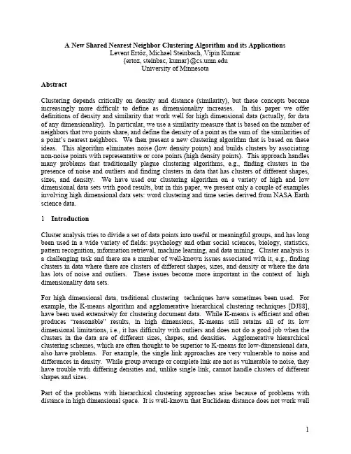
A New Shared Nearest Neighbor Clustering Algorithm and its Applications Levent Ertöz, Michael Steinbach, Vipin Kumar {ertoz, steinbac, kumar}@ University of Minnesota Abstract Clustering depends critically on density and distance (similarity), but these concepts become increasingly more difficult to define as dimensionality increases. In this paper we offer definitions of density and similarity that work well for high dimensional data (actually, for data of any dimensionality). In particular, we use a similarity measure that is based on the number of neighbors that two points share, and define the density of a point as the sum of the similarities of a point’s nearest neighbors. We then present a new clustering algorithm that is based on these ideas. This algorithm eliminates noise (low density points) and builds clusters by associating non-noise points with representative or core points (high density points). This approach handles many problems that traditionally plague clustering algorithms, e.g., finding clusters in the presence of noise and outliers and finding clusters in data that has clusters of different shapes, sizes, and density. We have used our clustering algorithm on a variety of high and low dimensional data sets with good results, but in this paper, we present only a couple of examples involving high dimensional data sets: word clustering and time series derived from NASA Earth science data. 1 IntroductionCluster analysis tries to divide a set of data points into useful or meaningful groups, and has long been used in a wide variety of fields: psychology and other social sciences, biology, statistics, pattern recognition, information retrieval, machine learning, and data mining. Cluster analysis is a challenging task and there are a number of well-known issues associated with it, e.g., finding clusters in data where there are clusters of different shapes, sizes, and density or where the data has lots of noise and outliers. These issues become more important in the context of high dimensionality data sets. For high dimensional data, traditional clustering techniques have sometimes been used. For example, the K-means algorithm and agglomerative hierarchical clustering techniques [DJ88], have been used extensively for clustering document data. While K-means is efficient and often produces “reasonable” results, in high dimensions, K-means still retains all of its low dimensional limitations, i.e., it has difficulty with outliers and does not do a good job when the clusters in the data are of different sizes, shapes, and densities. Agglomerative hierarchical clustering schemes, which are often thought to be superior to K-means for low-dimensional data, also have problems. For example, the single link approaches are very vulnerable to noise and differences in density. While group average or complete link are not as vulnerable to noise, they have trouble with differing densities and, unlike single link, cannot handle clusters of different shapes and sizes. Part of the problems with hierarchical clustering approaches arise because of problems with distance in high dimensional space. It is well-known that Euclidean distance does not work well1in high dimensions, and typically, clustering algorithms use distance or similarity measures that work better for high dimensional data e.g., the cosine measure. However, even the use of similarity measures such as the cosine measure does not eliminate all problems with similarity. Specifically, points in high dimensional space often have low similarities and thus, points in different clusters can be closer than points in the same clusters. To illustrate, in several TREC datasets (which have class labels) that we investigated [SKK00], we found that 15-20% of a points nearest neighbors were of a different class. Our approach to similarity in high dimensions first uses a k nearest neighbor list computed using the original similarity measure, but then defines a new similarity measure which is based on the number of nearest neighbors shared by two points. For low to medium dimensional data, density based algorithms such as DBSCAN [EKSX96], CLIQUE [AGGR98], MAFIA [GHC99], and DENCLUE [HK98] have shown to find clusters of different sizes and shapes, although not of different densities. However, in high dimensions, the notion of density is perhaps even more troublesome than that of distance. In particular, the traditional Euclidean notion of density, the number of points per unit volume, becomes meaningless in high dimensions. In what follows, we will define the density at a data point as the sum of the similarities of a point’s nearest neighbors. In some ways, this approach is similar to the probability density approach taken by nearest neighbor multivariate density estimation schemes, which are based on the idea that points in regions of high probability density tend to have a lot of close neighbors. While “better” notions of distance and density are key ideas in our clustering algorithm, we will also employ some additional concepts which were embodied in three recently proposed clustering algorithms, i.e., CURE [GRS98], Chameleon [KHK99], and DBSCAN. Although, the approaches of these algorithms do not extend easily to high dimensional data, they algorithms outperform traditional clustering algorithms on low dimensional data, and have useful ideas to offer. In particular, DBSCAN and CURE have the idea of “representative” or “core” points, and, although our definition is somewhat different from both, growing clusters from representative points is a key part of our approach. Chameleon relies on a graph based approach and the notion that only some of the links between points are useful for forming clustering; we also take a graph viewpoint and eliminate weak links. All three approaches emphasize the importance of dealing with noise and outliers in an effective manner, and noise elimination is another key step in our algorithm. To give a quick preview, our clustering approach first redefines the similarity between points by looking at the number of nearest neighbors that points share [JP73]. Using this similarity measure, we then define the notion of density based on the sum of the similarities of a point’s nearest neighbors. Points with high density become our representative or core points, while points with low density represent noise or outliers and are eliminated. We then find our clusters by finding all groups of points that are strongly similar to representative points. Any new clustering algorithm must be evaluated with respect to its performance on various data sets, and we present a couple of examples. For the first example, we find clusters in NASA Earth science data, i.e., pressure time series. For this data, our shared nearest neighbor (SNN) approach has found clusters that correspond to well-known climate phenomena, and thus we2have confidence that the clusters we found are “good.” Using these clusters as a baseline, we show that the clusters found by Jarvis-Patrick clustering [JP73], an earlier SNN clustering approach, and K-means clustering are not as “good.” For the second example, we cluster document terms, showing that our clustering algorithm produces highly coherent sets of terms. We also show that a cluster consisting of a single word can be quite meaningful. The basic outline of this paper is as follows. Section 2 describes the challenges of clustering high dimensional data: the definition of density and similarity measures, and the problem of finding non-globular clusters. Section 3 describes previous clustering work using the shared nearest neighbor approach, while Section 4 introduces our new clustering algorithm. Section 5 presents a couple of examples: the first example Section finds clusters in NASA Earth science data, i.e., pressure time series, while the second example describes the results of clustering document terms. 2 Challenges of Clustering High Dimensional DataThe ideal input for a clustering algorithm is a dataset, without noise, that has a known number of equal size, equal density, globular. When the data deviates from these properties, it poses different problems for different types of algorithms. While these problems are important for high dimensional data, we also need to be aware of problems which are not necessarily important in two dimensions, such as the difficulties associated with density and measures of similarity and distance. In this section, we take a look at these two problems and also consider the importance of representative points for handling non-globular clusters. 2.1 Behavior of similarity and distance measures in high dimensions The most common distance metric used in low dimensional datasets is Euclidean distance, or the L2 norm. While Euclidean distance is useful in low dimensions, it doesn’t work as well in high dimensions. Consider the pair of ten-dimensional data points, 1 and 2, shown below, which have binary attributes. Point 1 2 Att1 1 0 Att2 0 0 Att3 0 0 Att4 0 0 Att5 0 0 Att6 0 0 Att7 0 0 Att8 0 0 Att9 0 0 Att10 0 1If we calculate the Euclidean distance between these two points, we get √2. Now, consider the next pair of ten-dimensional points, 3 and 4. Point 3 4 Att1 1 0 Att2 1 1 Att3 1 1 Att4 1 1 Att5 1 1 Att6 1 1 Att7 1 1 Att8 1 1 Att9 1 1 Att10 0 1If we calculate the distance between point 3 and 4, we again find out that it’s √2. Notice that points 1 and 2 do not share any common attributes, while points 3 and 4 are almost identical. Clearly Euclidean distance does not capture the similarity of points with binary attributes. The problem with Euclidean distance is that missing attributes are as important as the present3attributes. However, in high dimensions, the presence of an attribute is a lot more important than the absence of an attribute, provided that most of the data points are sparse vectors (not full), and in high dimensions, it is often the case that the data points will be sparse vectors, i.e. they will only have a handful of non-zero attributes (binary or otherwise). Different measures, such as the cosine measure and Jaccard coefficient, have been suggested to address this problem. The cosine similarity between two data points is equal to the dot product of the two vectors divided by the individual norms of the vectors. (If the vectors are already normalized the cosine similarity simply becomes the dot product of the vectors.) The Jaccard coefficient between two points is equal to the number of intersecting attributes divided by the number of spanned attributes by the two vectors (if attributes are binary). There is also an extension of Jacquards coefficient to handle non-binary attributes. If we calculate the cosine similarity or Jaccard coefficient between data points 1 and 2, and 3 and 4, we’ll see that the similarity between 1 and 2 is equal to zero, but is almost 1 between 3 and 4. Nonetheless, even though we can clearly see that both of these measures give more importance to the presence of a term than to its absence, there are cases where using such similarity measures still does not eliminate all problems with similarity in high dimensions. We investigated several TREC datasets (which have class labels), and found out that 15-20% of the time, for a data point A, its most similar data point (according to the cosine measure) is of a different class. This problem is also illustrated in [GRS99] using a synthetic market basket dataset. Note that this problem is not due to the lack of a good similarity measure. Instead, the problem is that direct similarity in high dimensions cannot be trusted when the similarity between pairs of points are low. In general, data in high dimensions is sparse and the similarity between data points, on the average, is very low. Another very important problem with similarity measures in high dimensions is that, the triangle inequality doesn’t hold. Here’s an example: Point A B C Att1 1 0 0 Att2 1 0 0 Att3 1 1 0 Att4 1 1 0 Att5 1 1 0 Att6 0 1 1 Att7 0 1 1 Att8 0 1 1 Att9 0 0 1 Att10 0 0 1Point A is close to point B, point B is close to point C, and yet, the points A and C are infinitely far apart. The similarity between A and B and C and B comes from different sets of attributes. 2.2 Dealing with Non-globular Clusters using Representative PointsNon-globular cluster cannot be handled by centroid-based schemes, since, by definition, such clusters are not represented by their centroid. Single link methods are most suitable for capturing clusters with non-globular shapes, but these methods are very brittle and cannot handle noise properly. However, representative points are a good way of finding clusters that are not4characterized by their centroid and have been used in several recent clustering algorithms, e.g., CURE and DBSCAN. In CURE, the concept of representative points is used to find non-globular clusters. The use of representative points allows CURE to find many types of non-globular clusters. However, there are still many types of globular shapes that CURE cannot handle. This is due to the way the CURE algorithm finds representative points, i.e., it finds points along the boundary, and then shrinks those points towards the center of the cluster. The notion of a representative point is also used in DBSCAN, although the term “core point” is used. In DBSCAN, the density associated with a point is obtained by counting the number of points in a region of specified radius around the point. Points with a density above a specified threshold are classified as core points, while noise points are defined as non-core points that don’t have a core points within the specified radius. Noise points are discarded, while clusters are formed around the core points. If two core points are neighbors of each other, then their clusters are joined. Non-noise, non-border points, which are called boundary points, are assigned to the clusters associated with any core point within their radius. Thus, core points form the skeleton of the clusters, while border points flesh out this skeleton. While DBSCAN can find clusters of arbitrary shapes, it cannot handle data containing clusters of differing densities, since its density based definition of core points cannot identify the core points of varying density clusters. Consider Figure 1. If the user defines the neighborhood of a point by a certain radius and looks for core points that have a pre-defined number of points within that radius, then either the tight left cluster will be picked up as one cluster and the rest will be marked as noise, or else every point will belong to one cluster.neighborhood of a point Figure 1. Density Based Neighborhoods2.1.1Density in High Dimensional SpaceIn high dimensional datasets, the traditional Euclidean notion of density, which is the number of points per unit volume, is meaningless. To see this, consider that as the number of dimensions increases, the volume increases rapidly, and unless the number of points grows exponentially with the number of dimensions, the density tends to 0. Thus, in high dimensions, it is not5possible to use a (traditional) density based method such as DBSCAN which identifies core points as points in high density regions and noise points as points in low density regions. However, there is another notion of density that does not have the same problem, i.e., the notion of the probability density of a point. In the k-nearest neighbor approach to multivariate density estimation [DHS01], if a point that has a lot of close near neighbors, then it is probably in a region which has a relatively high probability density. Thus, when we look at the nearest neighbors of a point, points with a large number of close (highly similar) neighbors are in more “dense” regions than are points with distant (weakly similar) neighbors. In practice, we take the sum of the similarities of a points nearest neighbors as a measure of this density. The higher this density, the more likely it is that a point is a core or representative points. The lower the density, the more likely, the point is a noise point or an outlier. 3. Shared Nearest Neighbor Based Algorithm An alternative to a direct similarity is to define the similarity between a pair of points in terms of their shared nearest neighbors. That is, the similarity between two points is “confirmed” by their common (shared) near neighbors. If point A is close to point B and if they are both close to a set of points C then we can say that A and B are close with greater confidence since their similarity is “confirmed” by the points in set C. This idea of shared nearest neighbor was first introduced by Jarvis and Patrick [JP73]. A similar idea was later presented in ROCK [GRS99]. In the Jarvis – Patrick scheme, a shared nearest neighbor graph is constructed from the proximity matrix as follows. A link is created between a pair of points p and q if and only if p and q have each other in their closest k nearest neighbor lists. This process is called k-nearest neighbor sparsification. The weights of the links between two points in the snn graph can either be simply the number of near neighbors the two points share, or one can use a weighted version that takes the ordering of the near neighbors into account. Let i and j be two points. The strength of the link between i and j is now defined as: str (i, j ) = ∑ (k + 1 − m ) * (k + 1 − n ), where im = j n In the equation above, k is the near neighbor list size, m and n are the positions of a shared near neighbor in i and j’s lists. At this point, all edges with weights less than a user specified threshold are removed and all the connected components in the resulting graph are our final clusters [JP73]. Figures 2 and 3 illustrate two key properties of the shared nearest neighbor graph in the context of a 2-D point data set. In Figure 2, links to 5 most similar neighbors are drawn for each point. In Figure 3 shows unweighted shared nearest neighbor graph. In the graph, there is a link between points A and B, only if A and B had each other in their near neighbor lists.6Figure 2. Near Neighbor GraphFigure 3. Unweighted Shared Near Neighbor GraphThere are two important issues to note in this 2-D point set example. First, noise points and outliers end up having most of their links broken if not all. The point on the lower right corner ended up losing its entire links, because it wasn’t in the nearest neighbor lists of its own near neighbors. By just looking at the number of surviving links after constructing the snn graph, we can get rid of considerable amount of noise. Second, shared nearest neighbor graph is “density” independent, i.e. it will keep the links in uniform regions and break the ones in the transition regions. This is an important property, since widely varying tightness of clusters is one of the harder problems for clustering. A major drawback of the Jarvis – Patrick scheme is that, the threshold needs to be set high enough since two distinct set of points can be merged into same cluster even if there is only one link across them. On the other hand, if the threshold is too high, then a natural cluster may be split into too many small clusters due to natural variations in the similarity within the cluster. As a matter of fact, there may be no right threshold for some data sets. This problem is illustrated in the following example that contains clusters of points sampled from Gaussian distributions of two different means and variance. In Figure 4, there are two Gaussian samples. (Note that these clusters cannot be correctly separated by k-means due to the different sizes and densities of the samples). Figure 5 shows clusters obtained by Jarvis – Patrick method using the smallest possible threshold (any threshold smaller than this puts all points in the same cluster). Even this smallest possible threshold breaks the data into many different clusters. In Figure 5, different clusters are represented with different shapes and colors, where the discarded points / background points are shown as tiny squares. We can see that, even with a better similarity measure, it is hard to obtain the two apparent clusters.7Figure 4. Gaussian DatasetFigure 5. Connected Components - JP Clustering4. Shared Nearest Neighbor based Clustering Algorithm using Representative Points and Noise Removal In Section 3 we showed how Jarvis – Patrick method would fail on the gaussian dataset where transition between regions is relatively smooth. In this section, we present an algorithm that builds on Jarvis – Patrick method, and addresses the problems discussed in section 2. This algorithm uses a density based approach to find core / representative points. However, this approach will be based on the notion of density introduced in Section 2.3, which is based on the idea of probability density. However, since we will be using similarity based on a shared nearest neighbor approach, which automatically compensates for different densities (see Section 3), this density approach will not be subject to the same problem illustrated in Figure 1. 4.1 Noise Removal and Detection of Representative Points Figures 6-9 illustrate how we can find representative points and effectively remove noise using the snn graph. In this 2D point dataset, there are 8000 points. A near neighbor list size of 20 is used. Figure 7 shows all the points that have 15 or more links remaining in the snn graph. In Figure 8, all points have 10-14 links surviving and Figure 9 shows the remaining points. As we can see in these figures, the points that have high connectivity in the snn graph are candidates for representative / core points since they tend to be located well inside the natural cluster, and the points that have low connectivity are candidates for noise points and outliers as they are mostly in the regions surrounding the clusters. Note that all the links in the snn graph are counted to get the number of links that a point has, regardless of the strength of the links. An alternative way of finding representative points is to consider only the strong links in the count. Similarly we can find the representative points and noise points by looking at the sum of link strengths for every point in the snn graph. The points that have high total link strength then become candidates for representative points, while the points that have very low total link strength become candidates for noise points.8Figure 6. Initial Set of PointsFigure 7. Medium Connectivity PointsFigure 8. High Connectivity PointsFigure 9. Low Connectivity Points4.2 The Algorithm 1. 2. 3. 4. 5. 6. 7. 8. Construct the similarity matrix. Sparsify the similarity matrix using k-nn sparsification. Construct the shared nearest neighbor graph from k-nn sparsified similarity matrix. For every point in the graph, calculate the total strength of links coming out of the point. (Steps 1-4 are identical to the Jarvis – Patrick scheme.) Identify representative points by choosing the points that have high total link strength. Identify noise points by choosing the points that have low total link strength and remove them. Remove all links that have weight smaller than a threshold. Take connected components of points to form clusters, where every point in a cluster is either a representative point or is connected to a representative point.The number of clusters is not given to the algorithm as a parameter. Depending on the nature of the data, the algorithm finds “natural” clusters. Also note that not all the points are clustered using out algorithm. Depending on the application, we might actually want to discard many of the points. Figure 10 shows the clusters obtained from the Gaussian dataset shown in Figure 4 using the method described here. We can see that by using noise removal and the9representative points, we can obtain the two clusters shown below. The points that do not belong to any of the two clusters can be brought in by assigning them to the cluster that has the closest core point.Figure 10. SNN Clustering 5 Applications of SNN clustering5.1 Earth Science Data In this section, we consider an application of our SNN clustering technique to Earth science data. In particular, our data consists of monthly measurements of sea level pressure for grid points on a 2.5° longitude-latitude grid (144 horizontal divisions by 72 vertical divisions) from 1950 to 1994, i.e., each time series is a 540 dimensional vector. These time series were preprocessed to remove seasonal variation. For a more complete description of this data and the clustering analysis that we have performed on it, please see [Ste+01] and [Ste+02]. Briefly, Earth scientists are interested in discovering areas of the ocean, whose behavior correlates well to climate events on the Earth’s land surface. In terms of pressure, Earth scientists have discovered that the difference in pressure between two points on the Earth’s surface often yields a time series that correlates well with certain weather phenomena on the land. Such time series are called Ocean Climate Indices (OCIs). For example, the Southern Oscillation Index (SOI) measures the sea level pressure (SLP) anomalies between Darwin, Australia and Tahiti and is associated with El Nino, the anomalous warming of the eastern tropical region of the Pacific that has been linked to climate phenomena such as droughts in Australia and heavy rainfall along the Eastern coast of South America [Tay98]. Our goal in clustering SLP is to see if the difference of cluster centroids can yield a time series that reproduces known OCIs and to perhaps discover new indices.10longitudel a t i t u d e-30-60-901 2456789101112131415longitudel a t i t u d e-180-150-120-90-60-30 0 3060 90 120 150 180-30-60-9012456789101112131415longitudel a t i t u d e-180-150-120-90-60-30 0 3060 90 120 150 180906030 0-30-60-9052322212019181514131211109875421-60-30306090-90longitude631 K-means Clusters of SLP (1950-1994)17163Figure 12. JP clustering with optimal parametersFigure 11. SNN clusteringlatit ude906030 316 17 181920212223906030316 17181920212223Figure 14. K-means cluster after discarding “loose” clusters.Figure 13. JP clustering with sub-optimal parametersOur SNN clustering approach yielded the clusters shown in Figure 11. These clusters have been labeled (cluster “1” is the background or “junk” cluster) for easy reference. (Note that we cluster pressure over the entire globe, but here we focus on the ocean.) While we cluster the time series independently of any spatial information, the resulting clusters are typically geographically contiguous, probably because of the underlying spatial autocorrelation of the data.Using these clusters, we have been able to reproduce SOI as the difference of the centroids of clusters 13 and 10. We have also been able to reproduce another well-known OCI, i.e., NAO, which is the Normalized SLP differences between Ponta Delgada, Azores and Stykkisholmur, Iceland. NAO corresponds to the differences of the centroids of clusters 16 and 19. For more details, see [Ste+02]. This success gives us confidence that the clusters discovered by SNN have real physical significance.However, it is reasonable to ask whether other clustering techniques could also discover these clusters. To answer that question, we clustered the same data using the Jarvis-。
含羞草外形特征的描写作文英文回答:The Sensitive Plant, also known as Mimosa pudica, is an intriguing and visually captivating species withdistinctive morphological characteristics. Its foliage, stem, and flowers each possess unique features that contribute to its overall appearance.Foliage:The most striking aspect of the Sensitive Plant is its foliage. Its leaves are arranged alternately along the stem in a compound bipinnate structure. Each leaf consists of a central rachis, which bears pinnae on either side. These pinnae are further divided into leaflets, which are small, oblong-shaped structures. The leaflets are arranged in a mosaic-like pattern, giving the leaves an intricate and delicate appearance.The most remarkable attribute of the foliage is its sensitivity to touch. When a leaf isに触れる, its leaflets fold together rapidly, creating a distinctive closing motion. This phenomenon is known as seismonastic movement and is a defense mechanism that helps protect the plant from potential threats.Stem:The stem of the Sensitive Plant is slender and erect, growing up to a height of about 30 centimeters. It has a slightly hairy texture and is covered with small, hooked prickles. These prickles help support the plant and prevent herbivores from consuming it.Flowers:The flowers of the Sensitive Plant are small and inconspicuous, emerging from the axils of the leaves. They are arranged in dense, globular clusters, which are typically pink or purple in color. Each flower consists of a calyx of five sepals, a corolla of five petals, andnumerous stamens and pistils. The flowers are self-fertile, meaning they can produce seeds without the need for cross-pollination.The flowering period of the Sensitive Plant isrelatively long, extending from spring to fall. The flowers are visited by a variety of insects, including bees and butterflies, which aid in pollination.中文回答:含羞草,又名知羞草,是一种形态奇特、观赏性极强的植物,其叶、茎、花等各部分都具有独特的特征,共同构成其整体外形。
a rXiv:as tr o-ph/9711152v113Nov1997STELLAR POPULATIONS AND V ARIABLE STARS IN THE CORE OF THE GLOBULAR CLUSTER M51Laurent Drissen D´e partement de Physique and Observatoire du Mont M´e gantic,Universit´e Laval,Qu´e bec,QC,G1K 7P4Electronic mail:ldrissen@phy.ulaval.ca and Michael M.Shara Space Telescope Science Institute,3700San Martin Drive,Baltimore,Maryland 21218Electronic mail:mshara@ ABSTRACT We report the discovery of a variable blue straggler in the core of the globular cluster M5,based on a 12-hour long series of images obtained with the Planetary Camera aboard the Hubble Space Telescope .In addition,we present the light curves of 28previously unknown or poorly studied large-amplitude variable stars (all but one are RR Lyrae)in the cluster core.A (V,U-I)color-magnitude diagram shows 24blue stragglers within 2core radii of the cluster center.The blue straggler population is significantly more centrally concentrated than the horizontal branch and red giant stars.1.IntroductionGlobular cluster cores are being imaged intensively with the Hubble Space Telescope, and continue to yield surprises.The realizations that blue stragglers are commonplace,red giants are depleted,and that horizontal branch populations may depend on core properties has spurred on observers in the pastfive years.As part of our program to study the dis-tributions of blue stragglers and variable stars in globular cores,we have now imaged NGC 5904=M5.The globular cluster M5harbors one of the richest collections of RR Lyrae stars in the Galaxy.It is also home to one of only two known dwarf novae in Galactic globular clusters. Until now,however,not a single blue straggler candidate has been identified in M5.Is this because none exist,or because blue stragglers reside only in the(until now unobservable) core of M5?In section2we describe the observations and reductions;the CMD of the core of M5is presented in section3.The variable stars wefind are described in section4while our results are summarized in section5.2.Observations and reductions2.1.Search for variable starsA series of twenty-two600-second exposures of M5’s central(r≤50′′)region,spanning11.5hours,was obtained on March21,1993with the Planetary Camera(PC)aboard the Hubble Space Telescope(HST)before the repair mission.The F336Wfilter,similar to the Johnson U bandpass(Harris et al.al.1991),was used for the observations.Standard cali-bration(bias and dark subtraction,flatfield correction)was performed with STScI software within IRAF/STSDAS.The detection of variable stars was performed as follows.First,the22individual images were combined with IRAF’s combine task(with the crreject option)to create a deep image. This image is shown in Figure1.The individual images were remarkably well aligned with each other,so no shift was necessary.DAOPHOT’s Daofind algorithm(Stetson1987)was then used to build a masterlist of3144stars visible in the deep image.In order to eliminate the numerous cosmic rays,which are very difficult to remove on single frames,the22individual images were combined two by two(again with the combine task and the crreject option),with an overlap of1(image1+image2,image2+image3,...).Aperture photometry with an aperture radius of4pixels(0.17′′),and a sky annulus with inner and outer radii of10and15pixels was then performed on the21resulting images, using the masterlist of stars previously found.The standard deviation from the mean in the 21frames was then computed for all stars;this resulted in the discovery(or re-discovery)of 29variable stars,which will be discussed in section4.Note that since for any given star the conditions(PSF,flatfield,star location,aperture, background)are virtually identical from frame to frame(with the exception of faint stars near bright,large amplitude variables),the relative photometry from frame to frame is expected to be much more precise than the relative photometry among stars within the same frame (mostly because of PSF variations which induce position-dependent aperture corrections and overlapping PSFs in a crowdedfield).While the relative error from one star to the next within a single frame can be as large as0.2mag(if simple aperture photometry is used), even for bright stars,the typical standard deviation from the mean of the21frames for a given non-variable star is less than0.05mag at U=17.5,and reaches0.1mag at the cluster main sequence turnoff.2.2.The color-magnitude diagramIn order to study the stellar populations in M5,a70second F555W(equivalent of Johnson Vfilter;Harris et al.1991)and a70second F785LP(comparable to I)PC images were retrieved from the HST archives.Both images were obtained on December27,1991. Fortunately,the center of these frames is only∼8′′away from the center of our images (the totalfield of view of the4PC CCDs is70′′),so most stars detected in our F336W images are also located in the archive frames;the area common to all three sets of images is∼1.1arcmin2.Stellar photometry was performed in the most simple way on these frames:aperture photometry(with the same parameters as above)was performed on the deep,combined F336W frame using the masterlist.After proper shift and rotation of the coordinates,the same masterlist was used to obtain aperture photometry of the stars in the F555W and F785LP images.Although PSF-fitting techniques are known to improve the photometric accuracy(especially at the faint end of the luminosity function and near bright stars;see Guhathakurta et al.1992for a detailed discussion),simple core aperture photometry gives results which are reliable enough(typicallyσ∼0.2mag above the turnoff) for our purpose.A total of2153stars have been included in the color-magnitude diagram discussed below.Aperture corrections and photometric zero-points determined by Hunter et al.(1992) were used to calibrate the magnitudes and colors of the stars.Moreover,the absolute sen-sitivity of the CCDs is known to decrease slowly with time following each decontamination (Ritchie&MacKenty1993);this effect was taken into account.As a consistency check,the photometric calibration was compared with ground-based data.The average F555W and F336W magnitudes of the RR Lyrae stars are F555W RR= 15.2and F336W RR=15.55,while Buonanno et al(1981)find V RR=15.13and Richer& Fahlman(1987)obtained U HB=15.6.The agreement is excellent.3.Stellar PopulationsThe color-magnitude diagram for the2153stars located in the area common to the F336W(U),F555W(V)and F785LP(I)frames is shown in Figure2.In this plot,variable stars(see next section)are identified with special symbols;seven of29variables found in the F336W frames are located outside the F555W and F785LPfield of view,and are therefore not included in Figure2.Photometry is fairly complete down to∼0.5magnitude below the turnoff.The large wavelength difference between the U and Ifilters compensates for the relatively poor photometric accuracy,and allows us to clearly define the stellar populations. Two characteristics of the CMD are worth noting:the significant blue straggler population and the morphology of the horizontal branch.3.1.Blue StragglersThe boundaries of the BS region of the CMD have often been arbitrarily defined,vary from author to author,and also depend on thefilters used.As emphasized by Guhathakurta et al.(1994),the(V,U-I)CMD is well suited to define the blue straggler population.As a working definition,we decided to include in the BS region of the(V,U-I)CMD all stars significantly brighter(0.4mag)than the turnoffand bluer than the average main sequence at the turnofflevel;twenty-four stars are included in this region of the CMD(surrounded by dotted lines in Figure2)and can be considered as blue stragglers.Such a significant blue straggler population in the core of M5is in striking contrast to the outer regions of the cluster, where none have been found(Buonanno et al.1981,for2′≤r obs≤5.6′;Richer&Fahlman 1987,for3′≤r obs≤25′).Recent CCD observations of the central regions of M5(Brocato et al.(1995);Sandquist et al.(1996))also reveal some blue stragglers.The two-dimensional distribution of red giants,horizontal branch stars and blue stragglers is shown in Figures 3a-c.It is obvious from these plots that the BS population is preferentially concentrated in the very core of the cluster.This is quantified in Figure4a,which shows the cumulativedistribution of the different stellar populations within the inner50′′,and in Figure4b,within one core radius(24′′).A simple K-S test showed that there is a99.5%probability that the blue stragglers in the core of M5are more centrally concentrated than the horizontal branch stars,and a97.5%probability that they are more centrally concentrated than the red giants.This tendency for blue stragglers to be more centrally concentrated than other cluster members has been noted for most globular clusters observed to date(see Sarajedini(1993), Yanny et al.1994and references therein),and is consistent with the hypothesis that BS are more massive than main sequence stars.The luminosity-inferred lifetime of the shortest-lived,most luminous blue straggler in the core of M5is∼5×10⁸yrs,assuming it lies on the hydrogen-burning main sequence. This corresponds to the star with V=16.0,L∼25L⊙and M∼2.15M⊙.The relaxation time in the core of M5is T rc=2×10⁸yrs(Djorgovski1993).Hence,all BS in the core of M5are expected to be dynamically relaxed.Thus,the radial distribution of the BS is, indeed,a direct probe of their masses.In order to compare the blue straggler population from cluster to cluster,Bolte,Hesser &Stetson(1993)have defined the specific frequency,F BS,as the ratio of the number of blue stragglers to the total number of stars brighter than2magnitudes below the horizontal branch at the instability strip.In the case of the central region of M5(area in common to the U,V and I HST/PC frames),where V HB=15.2,24F BS=other clusters.He suggests that gaps may provide important constraints on mixing in earlier stages of stellar evolution.We see no evidence that the gap width changes between the inner and outer parts of the core.4.Variable StarsFigure5shows the standard deviation as a function of the average U magnitude for all the stars in the F336W frames.The usual problem with outliers in Figure5(due to mismatches in star lists)was almost completely avoided because(a)the same master list for all frames(see section2.1),and(b)all images were perfectly aligned with each other.Visual inspection of the few remaining outliers immediately showed them to be mismatches and they were eliminated from our photometry.Stars with RMS magnitude of variability higher than2sigma above the mean curve were considered possible variables and were examined more closely.Most of them were faint stars located close to bright,large-amplitude variables. Twenty-eight stars stand out as bright,large-amplitude variables in Figure5,as well as one fainter,low-amplitude variable star.Seven of these variable stars had never been identified previously,and two(HST-V20and V21)were considered as a single star.All but one of the large-amplitude variables have light curves typical of RR Lyrae stars,whereas the low-amplitude variable is a blue rmation on the variables,including cross-identification with previous papers,is presented in Table1.We note that the cataclysmic variable V101is36′′North and282′′West of the center of M5and is therefore too distant to have been included in thefield of view of the Planetary Camera(70′′×70′′).4.1.A Variable Blue StragglerOf24blue stragglers identified in Figure2,only one(HST-V28)shows evidence for variability above the noise level.Although only HST-V28showed up above the2-sigma variability level in Figure5,we have examined the light curve of every blue straggler and compared them with those of nearby stars of similar magnitude in order tofind possible variations undetected by our technique;no new variable showed up.But because the noise level is still relatively high between V=17and V=18(the2σvariability level varies from0.06 to0.12,corresponding to amplitudes∼0.2-0.3mag),we cannot exclude the possibility that some blue stragglers are actually small amplitude variables.The color-magnitude diagram(Figure2)shows that HST-V28is the bluest,and one of the brightest blue stragglers in M5(with M V=+2.2).Figure6shows its light curve,along with light curves of3nearby comparison stars of the same magnitude.HST-V28is obviously variable,with an amplitude∆U≥0.15mag.Unfortunately,our data do not allow us to determine the period with any precision(or even to determine if the variations are periodic).Phase dispersion minimization algorithms favor a periodicity of the order of ∼15hours(in which case this star could be an eclipsing binary),but cannot completely exclude periods shorter than∼1.9hours(typical for pulsating blue stragglers in clusters; Mateo1993).Better photometric accuracy and temporal sampling are obviously necessary to determine the period and nature of HST-V28.Guhathakurta et al.(1994)recently discovered2variables among the28blue stragglers in the core of M3.Both have photometric amplitudes∼0.4mag and periods∼6-12hours. Guhathakurta et al.suggest that both stars are dwarf cepheids.4.2.RR Lyrae StarsAmong the97genuine variables listed in Sawyer-Hogg’s(1973)catalogue,93are RR Lyrae.Recently,Kalda et al.(1987)and Kravtsov(1988,1992)searched for new variables in the central,crowded region of the cluster and found30more.So far,the light curves of only two of these new variables have been published(Kravtsov1992).A recent review of the M5RR Lyrae population has been published by Reid(1996).The U-band light curves of all RR Lyrae stars found in the HST images are shown in Figure7.Tentative periods have been determined for the9type RRc stars with a phase dispersion minimization algorithm,and the results are presented in Table1.The periods of RRab stars are too long to be determined from our observations alone.4.3.HST-V1Eclipsing binary stars are common in the periphery of M5’s core(Reid1996,Yan&Reid 1996),but star HST-V1is unique among the variables found in the core of M5.Although our observations do not cover an entire cycle(P∼0.55d−0.65d),the light curve suggests that HST-V1is a contact(or semi-detached)binary.The secondary minimum is very asymmetric, somewhat reminiscent of the near-contact binary V361Lyrae(Kaluzny1990).The strong asymmetry of the light curve of V361Lyr,more pronounced at shorter wavelengths,is thought to be caused by the presence of a hot spot on the secondary star resulting from the high mass transfer rate from the primary star.Unfortunately,HST-V1lies outside the boundaries of the F555W and F785LP frames, so its color cannot be determined.But with an average magnitude of U=15.7,HST-V1is more than two magnitudes brighter than the turnoff;if it is a cluster member,at least one of its components must be a giant.5.SummaryThe main results of our paper can be summarized as follows:(1)The core of M5contains a highly centrally concentrated population of blue stragglers, similar in size to that found in47Tuc(Paresce et al.1991).(2)Of24blue stragglers detected in the HST images,only one shows significant vari-ability above the noise level.Since our data are not sensitive enough to detect variables of amplitude≤0.2mag in the V=17-18range,we cannot exclude the possibility that some blue stragglers may be variable below that level.A more sensitive search with the refurbished HST is highly desirable.(3)We confirm the existence of a0.2mag gap in the color-magnitude distribution of the horizontal branch,first noted by Brocato et al..The nature of this gap is still unknown.(4)We have presentedfinding charts and light curves for27RR Lyrae variables and one probable contact binary.Among those variables,seven were previously unknown and21 had no published light curve.Support for this work was provided by NASA through grant number GO-3872from the Space Telescope Science Institute,which is operated by the Association of Universities for Research in Astronomy,Inc.,under NASA contract NAS5-26555.REFERENCESBolte,M.,Hesser,J.E.,&Stetson,P.B.1993,ApJ,408,L89Brocato,E.,Castellani,V.,&Ripepi,V.1995,AJ,109,1670Buonanno,R.,Corsi,C.E.,&Fusi Pecci,F.1981,MNRAS,196,435Djorgovski,S.G.1993,in Structure and Dynamics of Globular Clusters,ASP Conf.Ser., Vol.50,S.G.Djorgovski and G.Meylan,eds.,p.373Guhathakurta,P.,Yanny,B.,Schneider,D.P.,&Bahcall,J.N.1992,AJ,104,1790Guhathakurta,P.,Yanny,B.,Bahcall,J.N.,&Schneider,D.P.1994,AJ,108,1786 Harris,H.C.,Baum,W.A.,Hunter,D.A.,&Kreidl,T.J.1991,AJ,101,677Hesser,J.E.1988,IAU Symposium No.126,eds.J.E.Grindlay and A.G.Davis Philip,p. 65Hunter,D.A.,Faber,S.M.,Light,R.,&Shaya,E.1992,in Wide Field/Planetary camera Final Orbital/Science verification Report,ed.S.Faber(STScI,Baltimore),chap.12 Kaluzny,J.,1990,AJ,99,1207Kaluzny,J.,&Shara,M.M.1987,ApJ,314,585Kravtsov,V.V.,1988,Astron.Tsirk.,1526,6Kravtsov,V.V.,1992a,Sov.Astron.Lett.18(4),246Kravtsov,V.V.,1992b,Sov.Astron.Lett.17(6),455Kadla,Z.I.,Gerashchenko,A.N.,Jablokova,N.V.,&Irkaev,B.N.,Astron.Tsirk.,1502, 7Mateo,M.1993,in Blue Stragglers,ed.R.A.Saffer(ASP Conf.Ser.53),p.74 Paresce,F.,Meylan,G.,Shara,M.M.,Baxter,D.,&Greenfield,P.1991,Nature,352,297 Reid,N.1996,MNRAS,278,367Richer,H.B.,&Fahlman,G.G.1987,ApJ,316,189Sarajedini,A.1993,in Blue Stragglers,ASP Conf.Ser.,vol.53,ed.R.E.Saffer,p.14 Sawyer-Hogg,H.,1973,D.D.O.Pub.,Vol3.,No.6Yan,L.&Reid,I.N.1996,MNRAS,279,751Yanny,B.,Guhathakurta,P.,Schneider,D.P.,&Bahcall,J.N1994,ApJ,435,L59Fig.1.—Full HST/PCfield of view(70′′×70′′)of the central region of M5.This image is the average of twenty-two F336W(U-band)exposures.Variable stars and the cluster center are identified.-2-1012342019181716151413U-I Fig.2.—Color-magnitude diagram for the stars common to the U (F336W),V(F555W)and I(F785LP)frames.RR Lyrae stars,and the variable blue straggler are shown with special symbols.050010001500050010001500Fig. 3.—Distribution of the red giants,horizontal branch stars and blue stragglers in the V frame coordinate system.The location of the U images is shown.The cluster center is identified by a cross.The circle has a radius of 20′′(∼one core radius).050010001500050010001500Fig.3.—continued050010001500050010001500Fig.3.—continuedFig.4a.—(a)Cumulative distribution of the stellar populations (BS:Blue Stragglers;HB:Horizontal Branch stars;RG:Red Giants)in the inner 50′′region of M5;(b)same as (a),but within one core radiusFig.5.—The RMS magnitude of variability as a function of the F336W magnitudes for the stars in the21frame set.The line is the2σcutoff,above which the stars were considered as candidate variables and examined more closely.Genuine variables are shown with specialsymbols.Fig.6.—Light curve of HST-V28,the variable blue straggler and of three nearby(∆d≤5′′)comparison stars of similar mean magnitudeFig.7.—Light curves(filter F336W∼U-band)of the large amplitude variable stars found in the core of M5.All but one(HST-V1)are RR Lyrae stars.Fig.7.—ContinuedFig.7.—ContinuedFig.7.—Continued。
五年级天文知识英语阅读理解25题1<背景文章>The Sun is a very important star in our solar system. It is a huge ball of hot gas. The Sun is extremely bright and gives off a lot of heat and light. Without the Sun, life on Earth would not be possible.The Sun is made up of mostly hydrogen and helium. It is constantly undergoing nuclear reactions that release a tremendous amount of energy. This energy travels through space and reaches Earth, providing warmth and light for all living things.The Sun also has sunspots, which are areas that appear darker on the surface. Sunspots are caused by intense magnetic activity. Sometimes there are solar flares and prominences, which are powerful eruptions on the Sun.1. The Sun is mainly made up of ___.A. oxygen and nitrogenB. hydrogen and heliumC. carbon and oxygenD. nitrogen and carbon答案:B。
高二英语天文理解单选题40题1. The sun is the center of the solar system, and it is mainly composed of ____.A. oxygen and nitrogenB. hydrogen and heliumC. carbon dioxide and methaneD. water vapor and dust答案:B。
解析:太阳主要由氢(hydrogen)和氦(helium)组成。
选项A中的氧(oxygen)和氮(nitrogen)不是太阳的主要组成成分;选项C中的二氧化碳 carbon dioxide)和甲烷 methane)也不是;选项D中的水蒸气 water vapor)和尘埃 dust)同样不是太阳的主要组成部分。
2. Which planet in the solar system has the most visible rings?A. MarsB. JupiterC. SaturnD. Venus答案:C。
解析:在太阳系中,土星(Saturn)有着最明显的光环。
火星(Mars)没有光环,所以选项A错误;木星(Jupiter)虽然有光环但不如土星的明显,选项B错误;金星 Venus)没有光环,选项D错误。
3. The Earth is the only planet known to have ____ on its surface.B. liquid waterC. ammoniaD. sulfuric acid答案:B。
解析:地球是已知唯一表面有液态水(liquid water)的行星。
虽然地球两极有冰 ice),但这不是其区别于其他行星的唯一特征,选项A不准确;氨(ammonia)不是地球表面的典型物质,选项C错误;硫酸(sulfuric acid)也不是地球表面的常见物质,选项D 错误。
4. Which planet is closest to the sun?A. MercuryB. EarthC. VenusD. Mars答案:A。
焊缝射线照相底片的评判规律一、探伤人员要评片,四项指标放在先*,底片标记齐又正,铅字压缝为废片。
二、评片开始第一件,先找四条熔合线,小口径管照椭圆,根部都在圈里面。
三、气孔形象最明显,中心浓黑边缘浅,夹渣属于非金属,杂乱无章有棱边。
四、咬边成线亦成点,似断似续常相见,这个缺陷最好定,位置就在熔合线。
五、未焊透是大缺陷,典型图象成直线,间隙太小钝边厚,投影部位靠中间。
六、内凹只在仰焊面,间隙太大是关键,内凹未透要分清,内凹透度成弧线。
七、未熔合它斜又扁,常规透照难发现,它的位置有规律,都在坡口与层间。
八、横裂纵裂都危险,横裂多数在表面,纵裂分布范围广,中间稍宽两端尖。
九、还有一种冷裂纹,热影响区常发现,冷裂具有延迟性,焊完两天再拍片。
十、有了裂纹很危险,斩草除根保安全,裂纹不论长和短,全部都是Ⅳ级片。
十一、未熔和也很危险,黑度有深亦有浅,一旦判定就是它,亦是全部Ⅳ级片。
十二、危害缺陷未焊透,Ⅱ级焊缝不能有,管线根据深和长,容器跟着条渣走**。
十三、夹渣评定莫着忙,分清圆形和条状,长宽相比3为界,大于3倍是条状。
十四、气孔危害并不大,标准对它很宽大,长径折点套厚度,中间厚度插入法。
十五、多种缺陷大会合,分门别类先评级,2类相加减去Ⅰ,3类相加减Ⅱ级。
十六、评片要想快又准,下拜焊工当先生,要问诀窍有哪些,焊接工艺和投影。
注:*四项指标系底片的黑度、灵敏度、清晰度、灰雾度必须符合标准的要求。
**指单面焊的管线焊缝和双面焊的容器焊缝内未焊透的判定标准。
Radiograph Interpretation - WeldsIn addition to producing high quality radiographs, the radiographer must also be skilled in radiographic interpretation. Interpretation of radiographs takes place in three basic steps which are (1) detection, (2) interpretation, and (3) evaluation. All of these steps make use of the radiographer's visual acuity. Visual acuity is the ability to resolve a spatial pattern in an image. The ability of an individual to detect discontinuities in radiography is also affected by the lighting condition in the place of viewing, and the experience level for recognizing various features in the image. The following material was developed to help students develop an understanding of the types of defects found in weldments and how they appear in a radiograph.DiscontinuitiesDiscontinuities are interruptions in the typical structure of a material. These interruptions may occur in the base metal, weld material or "heat affected" zones. Discontinuities, which do not meet the requirements of the codes or specification used to invoke and control an inspection, are referred to as defects.General Welding DiscontinuitiesThe following discontinuities are typical of all types of welding.Cold lap is a condition where the weld filler metal does not properly fuse with the base metal or the previous weld pass material (interpass cold lap). The arc does not melt the base metal sufficiently and causes the slightly molten puddle to flow into base material without bonding.Porosity气孔is the result of gas entrapment in the solidifying metal. Porosity can take many shapes on a radiograph but often appears as dark round or irregular spots or specks appearing singularly, in clusters or rows. Sometimes porosity is elongated and may have the appearance of having a tail This is the result of gas attempting to escape while the metal is still in a liquid state and is called wormhole porosity. All porosity is a void in the material it will have a radiographic density more than the surrounding area..Cluster porosity链状气孔is caused when flux coated electrodes are contaminated with moisture. The moisture turns into gases when heated and becomes trapped in the weld during the welding process. Cluster porosity appear just like regular porosity in the radiograph but the indications will be grouped close together.Slag inclusions夹渣 are nonmetallic solid material entrapped in weld metal or between weld and base metal. In a radiograph, dark, jagged asymmetrical shapes within the weld or along the weld joint areas are indicative of slag inclusions.Incomplete penetration (IP) or lack of penetration (LOP)未焊透occurs when the weld metal fails to penetrate the joint. It is one of the most objectionable weld discontinuities. Lack of penetration allows a natural stress riser from which a crack may propagate. The appearance on a radiograph is a dark area with well-defined, straight edges that follows the land or root face down the center of the weldment.Incomplete fusion未熔合is a condition where the weld filler metal does not properly fuse with the base metal. Appearance on radiograph: usually appears as a dark line or lines oriented in the direction of the weld seam along the weld preparation or joining area.Internal concavity or suck back内凹或吸入is condition where the weld metal has contracted as it cools and has been drawn up into the root of the weld. On a radiograph it looks similar to lack of penetration but the line has irregular edges and it is often quite wide in the center of the weld image.Internal or root undercut内部或根部咬边is an erosion of the base metal next to the root of the weld. In the radiographic image it appears as a dark irregular line offset from the centerline of the weldment. Undercutting is not as straight edged as LOP because it does not follow a ground edge.External or crown undercut外部或顶部咬边is an erosion of the base metal next to the crown of the weld. In the radiograph, it appears as a dark irregular line along the outside edge of the weld area.Offset or mismatch错边are terms associated with a condition where two pieces being welded together are not properly aligned. The radiographic image is a noticeable difference in density between the two pieces. The difference in density is caused by the difference in material thickness. The dark, straight line is caused by failure of the weld metal to fuse with the land area.Inadequate weld reinforcement未填满is an area of a weld where the thickness of weld metal deposited is less than the thickness of the base material. It is very easy to determine by radiograph if the weld has inadequate reinforcement, because the image density in the area of suspected inadequacy will be more (darker) than the image density of the surrounding base material.Excess weld reinforcement增强余高is an area of a weld, which has weld metal added in excess of that specified by engineering drawings and codes. The appearance on a radiograph is a localized, lighter area in the weld. A visual inspection will easily determine if the weld reinforcement is in excess of that specified by the individual code involved in the inspection.Cracking裂纹can be detected in a radiograph only the crack is propagating in a direction that produced a change in thickness that is parallel to the x-ray beam. Cracks will appearas jagged and often very faint irregular lines. Cracks can sometimes appearing as "tails" on inclusions or porosity.Discontinuities in TIG weldsThe following discontinuities are peculiar to the TIG welding process. These discontinuities occur in most metals welded by the process including aluminum and stainless steels. The TIG method of welding produces a clean homogeneous weld which when radiographed is easily interpreted.Tungsten inclusions. 夹钨Tungsten is a brittle and inherently dense material used in the electrode in tungsten inert gas welding. If improper welding procedures are used, tungsten may be entrapped in the weld. Radiographically, tungsten is more dense than aluminum or steel; therefore, it shows as a lighter area with a distinct outline on the radiograph.Oxide inclusions夹氧化物are usually visible on the surface of material being welded (especially aluminum). Oxide inclusions are less dense than the surrounding materials and, therefore, appear as dark irregularly shaped discontinuities in the radiograph.Discontinuities in Gas Metal Arc Welds (GMAW)The following discontinuities are most commonly found in GMAW welds.Whiskers are short lengths of weld electrode wire, visible on the top or bottom surface of the weld or contained within the weld. On a radiograph they appear as light, "wire like" indications.Burn through (icicles) results when too much heat causes excessive weld metal to penetrate the weld zone. Lumps of metal sag through the weld creating a thick globular condition on the back of the weld. On a radiograph, burn through appears as dark spots surrounded by light globular areas.welld-02 (Incomplete Root Fusion、根部未熔合)—welld-03 (Insuffucient Reinforcement、增强高)——welld-04 (Excess Root Penetration、根部焊瘤)——welld-05 (External Undercut、外部咬肉)——welld-06 (Internal Undercut、内部咬肉)——welld-07 (Root Concavity、根部凹陷)——welld-08 (Burn Through、烧穿)——welld-09 (Isolated Slag Inclusion、单个的夹渣)——welld-10 (Wagon Track - Slag Line、线状夹渣)——welld-11 (Interrun Fusion、内部未熔合)——welld-12 (Lack of Sidewall Fusion、内侧未熔合)——welld-13 (Porosity、气孔)——welld-14 (Cluster Porosity、链状气孔)——welld-15 (Hollow Bead、夹珠)——welld-16 (Transverse Crack、横向裂纹)——welld-17 (Centerline Crack、中心线裂纹)——welld-18 (Root Crack、根部裂纹)——welld-19 (Tungsten Inclusion)夹钨—。
国家级新产品STAR—490 POS佚名【期刊名称】《中国经济和信息化》【年(卷),期】1995(000)0S1【摘要】<正> 性能 STAR—490 POS提供128K内存,支持ISO 8583数据格式;VISA Ⅰ/Ⅱ、SDLC、X.28通信格式;国际标准DES加密算法;异步/同步通信。
经国家科委、国家劳动部、国家技术监督局、国家外国专家局、中国工商银行认证,在技术上达到国际先进水平被评为国家级新产品。
外观由于公司对STAR—490 POS产品【总页数】1页(P58-58)【正文语种】中文【中图分类】N【相关文献】1.Sport and Doing Sports by the Disabled Post-traumatic Return to "Surge Et Ambula"(Get up and Walk), "Per Aspera Ad Astra"(Through Hardship to the Stars) [J], Miloslav Bardiovsky,;Romana Pitekowa;Zlata Ondrusova;Zuzana Gailikova;;;;;;;2.AG490对SD/Waistar大鼠心脏移植物的免疫抑制作用 [J], 王彬;朱绍兴;冯新顺;薛武军3.Poly(lactic acid)-starch/Expandable Graphite (PLA-starch/EG) Flame Retardant Composites [J], Mfiso Emmanuel Mngomezulu;Adriaan Stephanus Luyt;Steve Anthony Chapple;Maya Jacob John4.The fractions of post-binary-interaction stars and evolved blue straggler stars on the red giant branch of globular clusters [J], Dan-Dan Wei;Bo Wang;Hai-Liang Chen;Hai-Feng Wang;Xiao-Bo Gong;Dong-DongLiu;Deng-Kai Jiang5.Magstar推出Magstar Mobile POS移动POS [J],因版权原因,仅展示原文概要,查看原文内容请购买。
arXiv:astro-ph/0304434v1 24 Apr 2003Onthesizedifferencebetweenredandblueglobularclusters1SørenS.Larsen1andJeanP.BrodieUCObservatories/LickObservatory,UniversityofCalifornia,SantaCruz,CA95064,USA
slarsen@eso.organdbrodie@ucolick.org
ABSTRACTSeveralrecentstudieshavereportedameansizedifferenceofabout20%be-tweenthemetal-richandmetal-poorsubpopulationsofglobularclusters(GCs)inavarietyofgalaxies.Inthispaperweinvestigatethepossibilitythatthesizedifferencemightbeaprojectioneffect,resultingfromacorrelationbetweenclus-tersizeandgalactocentricdistance,combinedwithdifferentradialdistributionsoftheGCsubpopulations.Wefindthatprojectioneffectsmayindeedaccountforasizedifferencesimilartotheobservedone,providedthatthereisasteeprelationbetweenGCsizeandgalactocentricdistanceinthecentralpartsoftheGCsystemandthatthedensityofGCsflattensoffnearthecenterinamannersimilartoaKingprofile.Formorecentrallypeakeddistributions,suchasadeVaucouleursR1/4law,orforshallowersize-radiusrelations,projectioneffectsareunabletoproducetheobserveddifferencesinthesizedistributions.
Subjectheadings:galaxies:starclusters—Galaxy:globularclusters:general—galaxies:ellipticalandlenticular,cD
1.IntroductionSincetheworkofKinman(1959)andZinn(1985),ithasbeenknownthatglobularclustersintheMilkyWaycanbedividedinto(atleast)twosub-populationswithdistinct–2–kinematicalandchemicalproperties.Undoubtedlyoneofthemostimportantdevelopmentsinresearchonglobularclusters(GCs)withinthelastdecadeisthediscoverythatsimi-larsubstructureisseeninthecolor(andhence,presumably,metallicity)distributionsofGCsystemsinmanyearly-typegalaxies(Zepf&Ashman1993;Gebhardt&Kissler-Patig1999;Kundu&Whitmore2001;Larsenetal.2001).ThereisincreasingevidencethatGCsub-populationsinearly-typegalaxiessharemanypropertieswiththoseinspirals(Forbes,Brodie,&Larsen2001),andthattheGCsindifferentgalaxytypesmaybecloselyrelated.Characterizingandunderstandingtheproperties(spatialandmetallicitydistributions,kine-maticsetc.)ofGCsub-populationsiscurrentlyasubjectofmuchinvestigationandholdsthepromiseofrevealingimportantinformationabouteventsintheevolutionoftheirhostgalaxies.
OnepieceofthepuzzleistoestablishjusthowsimilarareGCsindifferentgalaxies.TheHubbleSpaceTelescopecanresolvethespatialprofilesofglobularclusterswellbeyondtheLocalGroup,althoughcarefulmodelingoftheundersampledpointspreadfunction(PSF)oftheWFPC2cameraisnecessaryinordertoderivereliablesizeinformationfortypicalextragalacticGCs.Kundu&Whitmore(1998)wereamongthefirsttomeasurethesizesofextragalacticGCsandfoundthatGCsinthelenticulargalaxyNGC3115hadhalf-lightradiiofabout2pc,similartoorperhapsslightlysmallerthanthoseintheMilkyWay.Whenmeasuringsizesfortheblue(metal-poor)andred(metal-rich)GCsubpopulationsseparately,Kundu&Whitmore(1998)notedasizedifferenceofabout20%withtheredGCsbeingsystematicallysmaller.AsimilarsizedifferencewasfoundbetweenredandblueGCsinNGC4486(Kunduetal.1999).Subsequently,sizedifferencesbetweenGCsubpopulationshavebeenfoundinmanyothergalaxiesincludingNGC4472(Puziaetal.1999),NGC4594(the“Sombrero”;Larsen,Forbes&Brodie2001),M31(Barmby,Holland,&Huchra2002)andotherearly-typegalaxies(Larsenetal.2001).However,itshouldalsobenotedthatHarrisetal.(2002)foundnosize-colorrelationforasampleof27GCsinNGC5128.
AlthoughtheresultsonNGC5128suggestthatthesizedifferencemaynotbeuniversal,thereseemstobecompellingevidencethatitisatleastawide-spreadphenomenon,observedinspiralsaswellasinearly-typegalaxies.Understandingtheoriginofthissizedifferenceisahighpriority,sinceanyintrinsiccorrelationbetweenthesizesandmetallicitiesofstarclustersmightholdcluestotheirformationmechanisms.However,beforeoneattemptstoexplainthesizedifferenceintermsofe.g.thepropertiesoftheproto-clusterclouds,variationsinexternalpressureetc.,othermorestraight-forwardexplanationsneedtoberuledout.
Onepossibilityisthattheobservedsizedifferenceisaprojectioneffect,resultingfromacorrelationbetweenGCsize(r)andGalactocentricdistance(R)combinedwithdifferentradialdistributionsoftheGCsubpopulations(throughoutthispaper,wewilladoptthe–3–followingconvention:asmallrreferstothesize(radius)ofanindividualglobularcluster,whileacapitalRreferstothedistanceofthatclusterfromthegalaxycenter.Wewillusesubscripts(Rproj,R3D)tospecifyprojectedand3-Dquantities).vandenBergh,Morbey,&Pazder(1991)foundthatthesize-RrelationintheMilkyWaycanbeapproximatedbyasquare-rootrelation,r∝√