Director, MSU Manufacturing Research Consortium
- 格式:pdf
- 大小:231.42 KB
- 文档页数:73
简介杨梦甦教授1984年毕业于厦门大学化学系,1993年获得加拿大多伦多大学博士学位,1993-1994期间在美国加州生物医学机构Scripps Research Institute从事研究工作。
1994年底加入香港城市大学,现任香港城市大学生物及化学系讲座教授和香港城市大学深圳生物医药中心主任,并兼任英国中兰开夏大学、浙江大学、解放军第三军医大学、沈阳药科大学、及解放军总医院客座教授。
在行政工作方面担任香港城市大学校董会荣誉学位委员会、大学顾问委员会、大学教务会、研究生院理事会等多个委员会成员。
杨教授主要研究领域为生物芯片技术的开发与应用和纳米生物领域的基础与应用研究, 1995年迄今成功获得包括国家高科技发展计划(863计划)、香港特区政府创新科技基金和研究资助局、及香港赛马会基金等逾6千万港元研究基金的资助,负责管理多个大型科研项目,亦是香港特区政府大学资助委员会之“药物发现与合成分子技术研究”、“中药基础研究与开发”、“海洋环境研究与创新技术”三个卓越学科的主要成员之一。
迄今在国际权威杂志共发表论文160余篇,专著章节17篇,在国内核心杂志发表论文50余篇,在大型国际会议共发表论文80余篇,应邀在各大学和研究机构做过逾70场学术报告,在相关领域申请/获得20多项中国及美国专利。
杨教授实验室已培训18名博士、8名硕士及16名博士后。
杨教授为香港特区政府创新科技基金评审委员会和健康防护基金评审委员会成员,及香港特区政府创新科技署纳米技术和先进材料研究院(NAMI)技术顾问,并兼任英国皇家化学会专业杂志《The Analyst》和中国化学会专业杂志《生命科学仪器》编辑委员会成员,德国《Microchimica Acta》国际顾问委员会成员,以及国际生物芯片大会学术委员会和世界华人高科技化学大会学术委员会成员。
杨教授从2002年主持筹建香港城市大学深圳生物医药中心,领导该中心成功获得包括国家高科技发展计划(863)课题及广东省科技重点攻关项目的资助,并得到深圳市/广东省政府的多次奖励,被授予深圳市生物芯片重点实验室的称号。
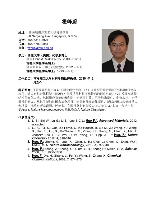
霍峰蔚地址: 新加坡南洋理工大学材料学院50 Nanyang Ave., Singapore, 639798电话: +65-6316-8921传真: +65-6790-9081电邮:fwhuo@.sg学历:西北大学(美国)化学系博士,师从Chad A. Mirkin院士,2009年12月吉林大学化学系硕士,师从张希院士和王治强教授,2002年5月吉林大学化学系学士,1999年5月工作经历:南洋理工大学材料学院助理教授,2010年2月至今科研简介: 目前课题组集中在以下两个研究方向:(1)多孔配位聚合物复合材料的研究与应用。
通过有机金属框架(MOFs)包覆功能材料实现特殊的催化性能。
(2)发展高通量纳米图案化方法,包括聚合物笔纳米印刷,光笔引刷等,用于纳米器件,生物芯片,光学器件的研究。
承担了新加坡国家基金项目、新美新能源合作项目、新以能源与水处理重大专项等一批重点研究课题。
近年来,在国外著名刊物发表SCI论文30多篇,包括一作Science, Nature Nanotechnology, 通讯联系人Nature Chemistry。
代表性论文:1. Li S.; Shi W.; Lu G.; Li S.; Loo S.C.J.; Huo F.*,Advanced Materials, 2012,accepted.2. Lu, G.; Li, S.; Guo, Z.; Farha, O. K.; Hauser, B. G.; Qi, X.; Wang, Y.; Wang,X.; Han, S.; Liu, X.; DuChene, J. S.; Zhang, H.; Zhang, Q.; Chen, X.; Ma, J.;Joachim Loo, S. C.; Wei, D. W.; Yang, Y.; Hupp, J. T.*; Huo, F.*NatureChemistry 2012, 4, 310-316.3. Huo, F.; Zheng, G.; Liao, X.; Giam, L. R.; Chai, J.; Chen, X.; Shim, W.Y.;Mirkin, C. A. Nature Nanotechnology, 2010, 5, 637-640.4. Huo, F.; Zheng, Z.; Zheng, G.; Giam, L. R.; Zhang H.; Mirkin, C. A. Science,2008, 321, 1658-1660.5. Huo, F.; Xu, H.; Zhang, L.; Fu, Y.; Wang, Z.; Zhang, X. ChemicalCommunications, 2003, 7, 874-875.。
爱考机构中国高端考研第一品牌(保过保录限额)爱考机构-北大考研-化学与分子工程学院研究生导师简介-杨娟杨娟博士,副教授纳米材料与纳米结构,分子光谱学电话:(010)62755357(办公室)Email:yang_juan@学术简历:1997-2001北京大学技术物理系,获理学学士学位;2001-2006TexasA&MUniversity,DepartmentofChemistry,获哲学博士学位(Advisor:Dr.JaanLaane);2006-2007TexasA&MUniversity,DepartmentofChemistry,博士后研究员(Supervisor:Dr.JaanLaane);2007-2008PacificNorthwestNationalLaboratory,博士后研究员(Supervisor:Dr.AllaZelenyuk);2009-2010北京大学化学与分子工程学院,讲师;2010-北京大学化学与分子工程学院,副教授。
研究领域和兴趣:采用分子光谱学研究方法,包括吸收光谱、拉曼光谱和荧光光谱等,对单壁碳纳米管的结构和性质进行表征,并结合分子动力学等理论模拟计算,获得有关碳纳米管电子性质与能带结构的信息。
具体研究项目如下:1)离子液体分散的单壁碳纳米管的本征光谱研究;2)离子液体分散的单壁碳纳米管与共轭分子等相互作用的光谱研究;3)单壁碳纳米管与生物大分子相互作用的表面增强拉曼光谱研究。
代表性论文:1.J.Yang,M.Stewart,G.Maupin,D.HerlingandA.Zelenyuk,Chem.Eng.Sci.,64,1625(2009);2.A.Zelenyuk,J.Yang,C.Song,R.A.Zaveri,andD.Imre,J.Phys.Chem.A,112,669(2008);3.J.Yang,M.Wagner,ane,J.Phys.Chem.A,111,8429(2007);4.J.Yang,J.Choo,O.Kwon,ane,Spectrochim.ActaPartA,68,1170(2007);5.ane,J.Mol.Struct.,798,27(2006);6.J.Yang,M.Wagner,K.Okuyama,K.Morris,Z.Arp,J.Choo,N.Meinander,O.Kwon,ane,J.Chem. Phys.,125,034308(2006);7.J.Yang,M.Wagner,ane,J.Phys.Chem.A,110,9805(2006);8.J.Yang,K.Okuyama,K.Morris,ane,J.Phys.Chem.A,109,8290(2005);9.J.Yang,K.McCann,ane,J.Mol.Struct.,695-696,339(2004).。
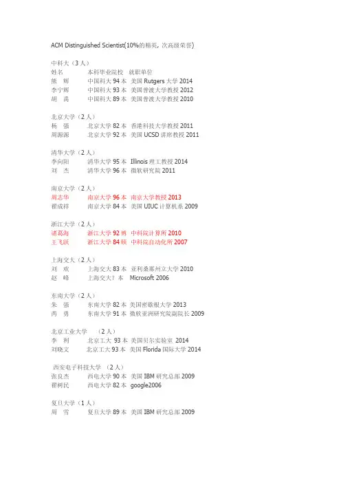
ACM Distinguished Scientist(10%的精英, 次高级荣誉)中科大(3人)姓名本科毕业院校就职单位熊辉中国科大94本美国Rutgers大学2014李宁辉中国科大93本美国普渡大学教授2012胡禹中国科大89本美国普渡大学教授2010北京大学(2人)杨强北京大学82本香港科技大学教授2011周源源北京大学92本美国UCSD讲席教授2011清华大学(2人)李向阳清华大学95本 Illinois理工教授2014刘杰清华大学96本微软研究院2011南京大学(2人)周志华南京大学96本南京大学教授2013翟成祥南京大学84本美国UIUC计算机系2009浙江大学(2人)诸葛海浙江大学92博中科院计算所2010王飞跃浙江大学84硕中科院自动化所2007上海交大(2人)刘欢上海交大83本亚利桑那州立大学2010赵峰上海交大?本 Microsoft2006东南大学(2人)朱强东南大学82本美国密歇根大学2013芮勇东南大学91本微软亚洲研究院副院长2009北京工业大学(2人)李利北京工大93本美国贝尔实验室2014刘晓文北京工大93本美国Florida国际大学2014西安电子科技大学(2人)张良杰西电大学90本美国IBM研究总部2009翟树民西电大学82本 google2006复旦大学(1人)周雪复旦大学89本美国IBM研究总部2009国防科大学(1人)朱文武国防科大85本清华大学教授2012其他王飞跃青岛科大82本中科院自动化所2007张良杰西安交大92硕美国IBM研究总部2008陈建二中南大学82本美国Notre Dame大学2014陈子仪武汉大学(80肄)美国Notre Dame大学2014徐常胜清华大学96博中科院自动化所2012(本科不详)现公职单位为国内高校全部用红标标出。
岳劲峰简历岳劲峰现任美国中田纳西州立大学杰宁琼斯商学院管理与市场系副教授(终身教授)(Associate Professor with tenure, Middle Tennessee StateUniversity)联系地址:Jinfeng Yue, Ph.D.Associate ProfessorDepartment of Management and MarketingJenning A. Jones College of BusinessMiddle Tennessee State UniversityMurfreesboro, TN 37132USAE-MAIL: jyue@电话:001-615-898-5126学历:1983年7月:北京大学地球物理专业;学士1989年4月:西北工业大学管理系统工程专业;硕士1995年7月:内布拉斯加大学卡尼分校工商管理学;工商管理硕士(MBA, University of Nebraska at Kearney, USA)2000年5月:华盛顿州立大学统计学;硕士(MS in Statistics,Washington State University, USA)2000年7月:华盛顿州立大学工商管理学;博士(Ph.D. in Business Administration, Washington State University, USA)工作经历:2006年8月- 至今:中田纳西州立大学管理与市场系;副教授(获终身教职);2001年8月- 2006年7月:中田纳西州立大学管理与市场系,助理教授2000年8月- 2001年7月:东南奥克拉荷马州立(Southeastern Oklahoma State University)大学管理与市场系,助理教授1995年8月- 2000年7月:华盛顿州立大学管理与运筹系;助教1994年8月-1995年7月:内布拉斯加大学卡尼分校经济系;助教科研教学获奖总结从事管理科学与运筹学方面的研究,主要研究方向包括有限信息情况下的决策理论;供应链管理;库存管理;质量管理;多目标决策模型。
【致谢】感谢参与编写和提供信息的以下校友:IhateBS strong根据美国US News 2013年美国大学排名前100的顺序统计,缺漏错误之处难免,请大家补充分为Full Professor(正教授)、Associate Professor(副教授)和Assistant Professor三类,其中前两类一般具有终身教职,不含解放前的清华学子,也含有极少数非tenure track教职人员,和已离职的人员,只列出,不计入统计总数。
共有在职Tenure track系列教职的共552人,其中95名正教授。
副教授207人另有部分著名实验室全职研究人员54人,非常不全。
----------------------------------------------------------------------------1,哈佛大学7林希虹Professor, 生物统计系,美国统计学会会士,统计学最高奖COPSS总统奖获得者1989年清华大学数学系学士,1994年华盛顿大学博士/xihong-lin/刘军Professor, 生物统计系,美国统计学会会士,统计学最高奖COPSS总统奖获得者1985-1986年清华大学数学系研究生/~junliu/Yiling ChenAssociate Professor of Computer Science1996年人民大学经济学学士,1999年清华大学金融硕士,2005年宾州州立大学信息科学技术博士/Wei-Dong YaoAssistant Professor of Psychiatry清华大学物理系学士,1998年爱荷华大学博士/Profiles/display/Person/4435Hesheng LiuAssistant Professor of Radiology at Harvard Medical School2003年清华大学生医工程系博士/martinos/people/showPerson.php?people_id=636Jinjun ShiAssistant Professor of AnaesthesiaThe Harvard Clinical and Translational Science Center2000年清华大学化学学士,德州农机大学博士/Profiles/display/Person/43651李全政Assistant Professor , Harvard medical school1992年浙江大学生医工程学士,1997年清华大学生医工程硕士,南加州大学博士/CAMIS/?page_id=1628----------------------------------------------------------------------------1,普林斯顿大学2琚诒光Robert Porter Patterson Professor,普林斯顿大学机械与航空工程系1986年清华大学工程力学系学士,1988年硕士,1994年日本东北大学博士/People_files/Ju-resume.htm//2014年7月开始王梦迪Assistant Professor in Operations and Financial Engineering2008年清华自动化学士,2013年MIT博士/research/news/archive/?id=11152********施一公(已辞职)Professor, 分子生物系,全球蛋白质学会Irving Sigal青年科学家奖获得者。
秦勇,兰州大学萃英特聘教授,博士生导师,材料科学与工程一级学科学科带头人,纳米科学与技术研究所所长。
主要从事纳米能源技术、功能纳米器件与自供能纳米系统领域的研究,在纳米能源技术领域积累了较多的经验。
三项关于纳米发电机的研究工作成为这一领域发展过程中的三个具有重大意义的研究进展,相应成果以三篇学术论文的形式发表在Nature系列期刊上,包括一篇第一作者Nature论文,一篇第一作者Nature Nanotechnology论文,一篇第二作者Nature Nanotechnology论文。
2009年获得美国陶瓷学会授予的2008年度陶瓷研究领域最有价值贡献奖Ross Coffin Purdy奖,2009年获得甘肃省自然科学奖三等奖。
学习工作经历:1995年9月至1999年7月:兰州大学材料科学系,学士;1999年9月至2004年6月:兰州大学物理学院,材料物理与化学专业,博士; 2004年7月至目前:兰州大学物理学院,先后任讲师、教授,创建纳米科学与技术研究所,从事纳米能源技术、功能纳米器件与自供能纳米系统领域的研究; 2007年4月至2009年9月:美国佐治亚理工学院王中林院士研究组先后做访问学者、博士后,从事纳米发电机的研究;2009年10月回国后立即带领研究团队搭建实验室,在完善实验条件的同时立足于现有条件积极开展纳米发电机与功能纳米器件方面的研究。
代表性学术论文:1. “Self-powered Nanowire Devices”S. Xu, Y. Qin, C. Xu, Y.G. Wei, R. Yang, Z.L. Wang, Nature Nanotechnology, 2010, 5, 366-373. (S. Xu, Y. Qin and C. Xu contribute equally)2. “Microfiber-Nanowire Hybrid Structure for Energy Scavenging” Y. Qin, X.D. Wang and Z.L. Wang, Nature, 2008, 451, 809-813. (Y. Qin and X.D. Wang contribute equally)3. “Power generation with laterally-packaged piezoelectric fine wires” R. Yang, Y. Qin, L.Dai and Z.L. Wang, Nature Nanotechnology, 2009, 4, 34-39.4. “Converting Biomechanical Energy into Electricity by Muscle Driven Nanogenerator” R. Yang, Y. Qin, C. Li, G. Zhu, Z.L. Wang, Nano Letters, 2009, 9(3), 1201-1205.获奖情况:1. 美国陶瓷学会Ross Coffin Purdy奖,秦勇,王旭东,王中林教授,2009年度获得,获奖工作:纤维基纳米发电机。
A Genetic Algorithm Approach toCompaction, Bin Packing, and NestingProblems
© Erik D. Goodman, Alexander Y. Tetelbaum, and Victor M. Kureichik1994, Michigan State University
July 12, 1994All Rights Reserved
Erik D. Goodman, Professor and Director
A. H. Case Center for Computer-Aided Engineering and ManufacturingDirector, MSU Manufacturing Research ConsortiumProfessor, Electrical Engineering, Mechanical EngineeringCollege of EngineeringMichigan State University
Alexander Y. Tetelbaum, President and Professor
International Solomon University (Kiev, Ukraine)Adjunct Professor, Electrical EngineeringCollege of EngineeringMichigan State University
Victor M. Kureichik, Professor
Taganrog State University of Radio-Engineering (Russia)Visiting Professor, Electrical EngineeringCollege of EngineeringMichigan State University
TECHNICAL REPORT # 940702CASE CENTER FOR COMPUTER-AIDED ENGINEERING AND MANUFACTURINGMICHIGAN STATE UNIVERSITYTABLE OF CONTENTS1. INTRODUCTION................................................ 11.1. Report Overview........................................... 11.2. Research Tools and Validation................................. 4
2. BACKGROUND................................................. 62.1. Introduction to Layout Compaction.............................. 62.2. Basic Definitions and Taxonomy of Compaction..................... 72.3. Algorithms for Compaction.................................... 82.3.1. Constraint-graph 1-D Compaction Algorithms................ 82.3.2. Two-dimensional compaction (2-D compaction)............... 122.3.3. Constraint-graph hierarchical compaction ................... 132.3.4. Wire length minimization [40,41] ........................ 142.4. Layout Approaches Based on Genetic Algorithms .................. 152.5. Bin Packing, Nesting and Compaction Using Genetic Algorithms ........ 172.5.1. 1-D Bin Packing.................................... 172.5.2. 2-D Bin Packing and Nesting ........................... 232.5.3. 3-D Bin Packing .................................... 302.5.4. Compaction ....................................... 322.6. Conclusions.............................................. 35
3. PROJECT DESCRIPTION.......................................... 533.1. Project Statement.......................................... 533.2. Goals Statement........................................... 533.3. The Approach ............................................ 543.3.1. The Representation................................... 543.3.2. The Genetic Operators................................ 563.3.3. The Fitness Function.................................. 583.3.4. The Parallel GA Architecture............................ 583.4. Sequence of Problem Refinement............................... 603.5. Contribution and Impact...................................... 62
4. BIBLIOGRAPHY................................................ 6311. INTRODUCTIONThis technical report is prepared to record the preliminary work carried out in beginninga research project on the solution of a group of related problems by means of Genetic Algorithms(GA’s). These problems include integrated circuit layout compaction, bin packing, and nesting.The principal problem is compaction, with the others serving to illuminate and guide thecompaction work, as well as possibly receiving benefits from new tools developed. Efficient andnear-optimal solution of the compaction problem will enhance the linkage between symbolic levelmodeling of the layout and the mask level design of hierarchical (fragment-based), ultra-fast, low-power analog and logic circuits. The research goals are to develop new methodologies,abstractions, and theory that lead to more efficiently defined and utilized Computer-Aided Design(CAD) algorithms and tools for compaction, bin packing and nesting. These new methodologieswill incorporate important improvements in the handling of the physical, technological, andoptimization aspects of compaction. More effective solution of the bin packing and nestingproblems can help to solve the compaction problem, as well as being valuable in their own rightfor many practical problems. This will be accomplished by defining a new approach to the useof Genetic Algorithms (GAs)--for the compaction, bin packing, and nesting problems.The research will concentrate mostly on the application area of high-speed, low-poweranalog and digital circuits with clock rates up to 20 GHz. In many applications in this highperformance area, dramatically reduced chip area and signal delays are important designrequirements. The technology area of interest is multi-chip modules (MCM) based on currentor advanced silicon and GaAs technologies [1]. These technologies have the potential to deliverimprovements in power management, low voltage operation, low crosstalk interconnects, andclock frequencies. The CAD area of concentration deals with the compaction, bin packing, andnesting problems and the solving of them based on GAs. These algorithms, using simpleencoding and recombination mechanisms, display complicated behavior, and they turned out tobe useful in solving some extremely difficult problems.