Dynamical and content evolution of a sample of clusters from z~0 to z~0.5

A Bibliography of Publications in The InternationalJournal of Supercomputer Applications,The International Journal of Supercomputer Applications and High-Performance Computing,and TheInternational Journal of High PerformanceComputing ApplicationsNelson H.F.BeebeUniversity of UtahDepartment of Mathematics,110LCB155S1400E RM233Salt Lake City,UT84112-0090USATel:+18015815254FAX:+18015814148E-mail:beebe@,beebe@,beebe@(Internet)WWW URL:/~beebe/12April2006Version1.32Title word cross-reference 3[GGS01].d=2[BRT+92].CH+H2 CH∗3 CH2+H[ASW91]. CuO2[SSSW91].K2[CBW95].N[SWW94]. -Body[SWW94].-D[GGS01]./I[CHZ02].0th[RAGW93].100[IHM87].10P[DD89].1917-1991[Mar91].2[DD89].200/VF[DD89].3[THL88].3-D[THL88].3.0[BRM03]. 3090[DD89].3090-200[DD89].3090-200/ VF[DD89].31G*[PUR94].3800[WOG95].125[HRM89].5/SE[KJH96].6[PUR94].6-31G*[PUR94].90[DL97].A&M[Nas92].Access[WHL03]. Accessing[HLP+03].Accurate[TMWS91].Acoustic[GKN+96]. Active[Her91].Ad[BG02].Ada[Kok88]. Adapting[DE03].Adaptive[AH93]. Additive[PR95].Administration[SDA+01].Adsorption[CH94].Advances[KKDV03]. Aerodynamics[YM91].Agents[QWIC02]. agricultural[SH93].Aided[MM90].AIX[Ano01a].Alamos[BBB+91b]. Algebra[GJM88].Algorithm[GJM88]. Algorithms[KL87].All-to-All[BJ92]. Alliant[DD91].Allocation[WPBB01]. alpha[TKSK88].Amdahl[HE01].amines[PUR94].ammonium[PUR94]. Amplitude[BGK+90].analogs[PUR94]. Analysis[MB87,LS90].Analytic[MA89]. Analyze[KKCB98].Analyzers[Ano01a]. Analyzing[WPBB01].Anatomy[YFH+96].Animal[UB95]. animated[LSS93].Animation[SS89]. Aperture[MPG93].API[BH00]. Appendix[Ano01a].Appendixes[Ano01a].AppLeS[SBWS99]. Application[NKR90].Applications[Ano98a].Applied[vL+03]. Applying[Dem90].Approach[FBW87]. Approximate[Cho01].Aqueous[PRT90]. Architectural[Gro03].Architecture[Ish91].architectures[JO92].Area[DFP+96]. ARION[HLP+03].Arising[Ma00]. Arithmetic[BSB89].Army[Aus92].array[JO92].Arrival[Wit92].Aspects[ZOF90].Assessing[ACM88]. Assessment[ZOF90].Assist[BB02]. asynchronous[PH91].Atmosphere[HAF+96].Atmosphere-Ocean[HAF+96]. Atmospheric[ARR99].Atomic[IHM87]. Attributes[Del93].Automata[RE87]. Automatic[Cza03].Automobile[HTSK90].Autonomous[SKB01].Availability[Pra01].Aware[YBA+03]. Axisymmetric[SG91].B[Ano01a].Band[Tho90].Based[Nak99]. Basic[JO92,Don02a].Bay[WLVL+96]. Beamforming[CYT+02].Bearing[FFNP97].Behavior[AK93]. Benchmarking[BRT+92].Benchmarks[BCK89,BBB+91a].Benefits[ACM88].Beowulf[SS99].Best[Lee03].Beyond[SBF90].Binary[DIB00].Biofluid[RKKC90]. Biological[WW92].Biology[SSNM92]. Biomembranes[SABK94].BLAS[DD89]. Blast[Don02a].Block[BS88].Body[TMWS91].Bone[HOPB92]. Boundary[SG91].Bridging[SS99]. Broadcast[BJ92].Builder[DL97]. Building[Wit92].Bulk[DGP+97].Butterfly[Kum89].C[Poz97].C90[ABF+99].Cache[MBW87].Cache-Coherent[Wad99].Cactus[AAF+01].Calculation[ACG+90]. Calculational[ZOF90].calculations[TKSK88].Caltech[Din91]. Caltech/JPL[Din91].Campus[GNTLH97].Campus-Wide[GNTLH97].Can[Pan97]. Cancers[GKB93].Capacity[BL99]. Carcinogens[HB90].Cards[Gro03]. Carlo[MB87].Carolina[LC90].Case[WGI90].CBVE[WLVL+96]. CEBAF[DZDR95].Center[All88,BBW90].Centers[All88]. CFD[GKMT00].CGNR[Man97].3Challenge[Kit90].Changing[MMS88]. Characterization[LPJ98].Chemical[TW87].Chemically[MYC92]. ChemIO[NFK98].Chemistry[EDS95]. Chesapeake[WL VL+96]. Chromodynamics[Liu90].Circular[AEPR92].Circulation[KM95]. CLAS[DZDR95].Classification[Tho90]. Climate[WHL03].Climatic[WBMY90]. Clouds[Tho90].Club[BCK89].Cluster[KT99].Clustering[NRR97]. Clusters[DT99].CM[CC95].CM-2[CC95].CM-5[KJH96].CM-5/SE[KJH96].CM2[CH94].Co[Mat03].Co-reservation[Mat03].Co-scheduling[Mat03].Coarse[BGB+96]. Coarse-Grained[BGB+96].Code[MSK92].Codes[IHM87].Coherent[Wad99].Collaborative[NBB+96].Collaboratory[YFH+96].Collapse[HTSK90].Collections[HLP+03]. Collide[NBB+96].Color[Tho90].Color/ Albedo[Tho90].Combining[Gir02]. Communication[BBDR95]. Communication/Computation[BBDR95].Community[HBSM03].Comparative[MOK00].Comparing[BF01].Comparison[Gen88]. Comparisons[Ma00].Compilers[Ano01a]. Complete[LK01].Complex[GKB93]. Complexity[BGB+96].Component[KBA00].Compositional[KR94,KR95]. Compounds[FWZ91].Compression[DLY+98].Computation[Her88,TR92]. Computational[FBW87].Computations[Duk91].Computer[TW87].Computer-Aided[MM90].Computers[Meu88].Computing[Ewi88,Lee03].Concurrent[MBW87].Conference[KKDV03].Configuration[AEPR92].Confined[ACG+90].Conjugate[Mel87]. Connection[HZ91].Conquer[Cza03]. Constant[MP94].Constrained[NKR90]. Constraints[GSHL03].Contaminant[ABF+99].Context[YBA+03].Context-Aware[YBA+03].Contributors[Ano96b].Control[AK91]. Controlled[DSD+91].convex[SH93]. Coordinate[YRA+02].Coordinated[FP02].CORBA[P´e r03]. Correspondence[IS96].Cortical[WW92]. Coscheduling[BL99].Coupled[HAF+96]. Coupling[P´e r03].CPU[BL99].Crash[HTSK90,CEL+97].CRAY[THL88].CRAY-2[DD89].CRAY-T3E[Ma00].Creutz[BRT+92]. CRPC[CDP+94].Crystal[Cla91]. Crystallography[CTH+93].CUMUL VS[GKP97].CYBER[ABA87]. CYDRA[HRM89].CYDRA-5[HRM89]. D[THL88].DAMPVM[Cza03]. DAMPVM/DAC[Cza03].Data[KBH88]. Data-Intensive[KUE+00].Data-Parallel[HJ96].Dataflow[ACM88]. Datasets[SE92].Davidson[UF89]. Dealing[GSHL03].Debuggers[Ano01a]. Decomposition[Meu88].Decoupled[PH91].Dedicated[GSHL03]. Delay[Rao02].demand[dPIdA03].Dense[Ede93].Department[Kit90]. Deployable[GCL93].Deployment[GCL93].Deposition[MD99]. derivatives[Haj93].Design[GJM88]. Detailed[EDS95].Detector[DZDR95]. Determination[KBH88].Determined[CGB+94].Development[HRM89].device[Lai93]. Devices[RKKC90].Diagrams[FWZ91]. Dielectric[ZOF90].Difference[THL88].4Differential[Meu88].Diffusion[TW87]. Digital[MPG93].dimensional[KS89]. Dimensionality[BFLL99].Dimensions[TW87].Dip[LT90].Direct[CM97].Direction[Mah90]. Directions[Fol90a].Discharge[YW93]. Discovery[AAF+01,AEG+03].Discrete[Ham91].Disk[KNP87]. Disordered[KVY+90].Dissemination[GL97].Dissolution[Cla91].Distance[HME90]. Distributed[MW AR87].Distributed-Memory[MCW+00]. Distributing[CBSB01].Divide[Cza03]. Divide-and-Conquer[Cza03].DNA[HB90].DOE[HBSM03].Domain[Meu88].Domain-Specific[CDH+97b].Double[PRT90].Drive[HE01].Driven[CHZ02].Dual[Ish91].Dual-Level[BBC+00].DV[TKSK88].DV-X[TKSK88].Dynamic[ABA87]. Dynamical[FBW87].Dynamics[Gen88]. e-Science[HWP03].Early[HGD91]. Econometric[Pet87].Economic[NKR90]. Economics[AK91].Eddy[CK01].Editor[dA03].Editorial[Don92]. Education[Mah90].Effective[BCK89].Effects[WBMY90,Haj93].Efficiency[ABA87].Efficient[Mel87]. Eigenvalue[UF89].Eigenvalues[KC92]. Electromagnetic[DGP+97].Electron[KVY+90].Electronic[FWZ91]. Electroweak[BGK+90].Element[KM95]. Eliminating[HME90].Embedded[KK01]. Embedded/Real[KK01].Embedded/ Real-Time[KK01].Enabled[CD97]. Enabling[FKT01].Encoding[DLY+98]. End[Rao02].End-To-End[Rao02]. Endangered[BB02].energies[PUR94]. Energy[IHM87,Kit90].Engineering[MMS88].Enhancement[AAC+97].Enhancements[BDG+95].Entity[BGF02].Entropy[CBW95]. Environment[CCH+88,WL VL+96]. Environmental[DLY+98].Environments[MA89].Equation[Fro91]. Equations[Syz87].Equilibration[NKR90].Equilibrium[NK89].Erratum[KR95]. estimation[SH93].ETA[DD89].ETA-10P[DD89].EuroPVMMPI[KKDV03].Evaluate[WGI90].Evaluating[BBDR95]. Evaluation[BCK89].Event[NRR97]. Events[BG00].Evolution[WJS+90]. Exact[ZK93].Example[NBB+96]. Excited[WLC91].Excited-State[WLC91].Excitement[RAGW93].Expand[GCCC+03].Expect[Pan92]. Experience[HGD91].Experiences[Reu92].Experiment[HME90].Experimental[KL87].Experiments[AK91].Exploration[KPM+96].Exploring[HAF+96].Expression[RS03]. Expressions[BBDR95].Extreme[KC92].F ACOM[IHM87].Factor[DH96]. Factorization[DD89].factorizations[DEKL92].Farming[CKPD99].fast[TKSK88,KNP87].Fault[GKP97]. Faulty[LK01].Feasibility[KR94]. Feature[PTGB02].features[PUR94]. February[Sci92].Feedback[CGB+94]. Feedback-Scaling[CGB+94].Fermions[ZK93].Fernbach[Mar91]. FETI[GCD97].FFT[Wad99].FFT-Based[GGS01].field[PUR94].File[GCCC+03].Film[MD99].Financial[HZ91].Fine[ACM88].Fine-Grain[ACM88].Finite[THL88]. Finite-Element[MS02].First[DQFW90].5Flames[SG91].FLO67[WLB92].Floating[BSB89].Flow[HKK88].Flowfield[MKG90].Flows[MYC92].Fluid[Gen88].Fluid-Structure[KT99]. Fluorinated[DFC90].Fock[KKCB98]. force[PUR94].Forming[CM97].Fortran[KR94].Forum[Don02a]. Forward[THL88].Foundation[Web91]. Four[Tho90].Four-Band[Tho90].Fourier[KNP87].FPS[LT88].Fracture[BG00].Framework[vL+03]. Frankenstein[Wit92].Frontwidth[MBW87].Fueling[Her91]. Fujitsu[Ish91].Full[AEPR92].Fully[YW93].Fun[RAGW93].Function[ZOF90].Fundamental[MR90]. Fusion[ACG+90].Future[BSB89].FX[DD91].FX/80[DD91].Galaxies[Her91].Games[EGMP93].Gap[SS99].Gas[MKG90].Gases[WBMY90].Gauge[Mor89a].Gene[RS03].Generation[DE03].Genetic[RS03].GFLOP[SBF90].Glass[YSN90].Global[WBMY90]. Globalized[GKMT00].Globally[SH93]. Globus[FK97].GloVE[dPIdA03].Glow[YW93].Gluons[BRE+90]. Goodput[BL99].Gradient[Mel87]. Gradient-like[CSV91].GrADS[BCC+01]. Grain[ACM88].Grained[BGB+96]. Grand[Kit90].Graphs[LK01]. Gravitational[SWW94].Gravity[Ham91]. Greenbook’[HBSM03].Greenhouse[WBMY90].Grid[CKPD99,FKT01].Grid-based[LM03].GridLab[A+03]. Grids[DT99,vL+03].Groundwater[MMD98].Growth[Cla91]. Guest[dA03].Guided[F+03].Gyrofluid[KPM+96].Hadron[Liu90].Harbor[BBC+00]. Hartree[KKCB98].Hartree-Fock[KKCB98].Head[GKB93]. Heavy[Reu92].Heavy-Ion[Reu92]. Helium[Fro91].Helix[PRT90]. Helmholtz[BEF+95].Heterogeneous[RAGW93].Hierarchical[GJM88].High[THL88]. High-Level[BCC+01].High-Order[CC95].high-performance[Fer90].High-Pressure[WLC91].High-Wave[BEF+95].Higher[Mah90]. Highly[Sim90].history[Bra91].Hitachi[WOG95].Hoc[CHZ02,BG02]. Homotopy[DZRS99].Hoshen[CBZ97]. Hoshen-Kopelman[CBZ97].Hosted[HBSM03].HPCC[CBB+96].HPF[DL97].HPF-Builder[DL97]. HPVM[CLP+99].HPVM-Based[CLP+99].Hybrid[MS02]. Hyperbolic[FG97].Hypercube[Din91,KL87].Hypercubes[LK01].I-W AY[DFP+96].I/O[PH91].IBM[DD89].Ice[ZOF90].IceT[GS99]. IEH[LK01].II[JP93].IJSGA[Hua03]. ILU[Ma00].Image[AAC+97].Imaging[CBB+96].Immersive[THC+96]. Impact[GJM88,KBH88].Implementation[Mel87]. Implementations[RR96].Implementing[YFH+96].Implications[RE87].Implicit[GKMT00]. Improving[BL99].Incomplete[IIJ93]. Increased[WBMY90].Increasing[WW92].Index[Ano96a]. Industrial[DGP+97].Inequality[NK89]. Infer[RS03].Influence[Ede93]. Information[Ano96b].Information-Driven[CHZ02]. Information-Theoretic[FWSW02]. Infrastructure[FK97].Initial[WLVL+96]. Initio[ASW91].Institute[IHM87]. Instruction[HRM89].6Instrumentation[TM99].Integer[Gro03]. Integrate[BFLL99].Integrated[CFK+94]. Integration[QWIC02].Intel[KL87]. Intensive[Mah90].Inter[FWZ91].Inter-Semiconductor[FWZ91]. Interaction[Liu90].Interactions[TMWS91].Interactive[SS89].Interface[Ano94,SLG95].Interleaving[KNP87].International[Ano98a].Internet[Rao02]. Interpretation[Fei99].Introduction[Nag93].Inverse[Cho01]. Investigation[CK01].Investigations[Mav02].Ion[Reu92].iPSC[HGD91,KR95].iPSC/860[HGD91,KR95].Irregular[Man97]. Ising[BRT+92].Issue[Fol90b].Issues[MBW87].Iterated[RR96]. Iterative[MC90].Japan[IHM87].Jini[Hua03].Jini-based[Hua03].Jumpshot[ZLGS99]. Jupiter[Tho90].Kernel[TM99].Kinetics[ARR99]. knowledge[KT94].Kopelman[CBZ97]. Krylov[GKMT00].Kutta[RR96]. Laboratory[BBB+91b].Laminar[SG91]. Language[Sha88].languages[JO92]. Large[FBW87].Large-Scale[Ewi88]. Lattice[Mor89a].Law[HE01].LBLAS[KJH96,JO92].Learning[AH93]. Legion[GNTLH97].Length[DLY+98]. Level[DD89].Libraries[DMT01].Library[CE00,Poz97].Ligature[KBA00]. like[CSV91].Limited[TW87].Linda[SSNM92].Line[LWOB97].Linear[AGL87].Link[TLG98,Pet87]. Linux[Ano01a].Liquid[DQFW90]. Livermore[WGI90].Local[BRT+92,JO92].Local-Creutz[BRT+92].Localization[CYT+02].Localized[WCE95].Logical[SR98].Long[HRM89].Looking[AK93].Loop[IS96].Loops[WGI90].Loss[ZOF90].LU[DD89].Machine[SS89,LPG88].machines[KS89]. Magnetically[ACG+90]. Magnetohydrodynamic[ACG+90]. making[KT94].Man[Wit92]. Management[HTSK90].Many[TMWS91].Many-Body[TMWS91]. Mappings[PTGB02].Market[NK89]. Market-Based[WPBB01].Markets[IIJ93].Massively[Mon89]. Matching[ZC92].Materials[KVY+90]. Mathematical[Mon89].Matrices[KC92]. Matrix[AGL87].MCell[CBSB01].MCHF[SYF96].Means[BRT+92]. Mechanics[Her88].Mechanism[DZRS99]. Medicine[SSNM92].Meetings[Ano98c]. Member[HTSK90].Memoriam[Mar91]. memories[TKSK88].Memory[MBW87]. Merging[YBA+03].Mesh[WCE95].Mesh-Iterative[MCW+00].Meshes[Ytt97].Meso[GGS01].Meso-Scale[GGS01].Message[Ano94,SLG95].Message-Passing[Ano94,SLG95]. Metacomputing[FK97].Metals[Cla91]. Metascheduling[Mat03].method[TKSK88].Methods[Mel87]. Metric[HE01].MHD[ACG+90]. Microprocessors[WT99].Microscopic[YFH+96].Microtasked[MSK92].Microtasking[HA91].Middleware[CKPD99].Migration[KL87]. MIMD[BOD+91].Mini[Gen88].Mini-Supercomputers[Gen88]. Minimization[Rao02].Minnesota[Aus92].MiPAX[HKK88]. Missions[SKB01].MM2[PUR94].Mobile[FP02].Model[ABA87].7Modeled[WJS+90].Modeling[DD87]. Models[Pet87].Modern[BDG+00].Modified[HB90].Modulo[Gro03]. Molecular[DFC90].Monitoring[L WOB97].Monte[MB87]. Motions[DFC90].Moveout[LT90].MP[LT88].MP/416[THL88].MPI[Ano94].MPI-OpenMP[MS02]. MPI2[MPI98].MPICH[GL97].Much[RAGW93].Multiblock[Ytt97]. Multibody[BGI+99].Multicommodity[NK89].Multicomputer[Man97].Multicomputers[MOK00]. Multidimensional[HL W00]. Multidisciplinary[BGB+96].Multifrontal[MBW87].Multigrid[DMT97].Multilevel[DW97]. Multimodal[FWSW02].Multiparadigm[AS00].Multiphase[ZC92].Multiphysics[MCW+00].Multiple[Mor89b].Multiprocessing[YM91].Multiprocessor[BS88].Multiprocessors[DD91]. Multiprogramming[MA89].Multitasking[THL88].Multiunit[GCL93].NAMD[NHG+96].Nanophase[Nak99]. NAS[BBB+91a].National[BBB+91b,All88].Navier[SBF90].Navier-Stokes[SBF90]. nCube[CL95].NEC[Mor89a].Neck[GKB93].Needs[HBSM03].NERSC[HBSM03].Net[AEG+03]. Netlets[Rao02].NetSolve[CD97]. Network[NZ93].Network-Based[AM00]. Network-Enabled[CD97].Networked[FWSW02].Networks[RE87]. Neural[RE87].Newton[GKMT00]. Newton-Krylov-Schwarz[GKMT00]. Next[DE03].NMR[KBH88].NOE[CGB+94].NOE-Restrained[CGB+94].Non[GSHL03].Non-Dedicated[GSHL03]. Nonequilibrium[YW93].Nonlinear[ABA87].Nonsymmetric[MC90].normal[Haj93]. North[LC90].Northern[UB95].Novel[FWZ91].NSF[Bra91].NT[CLP+99].Nuclear[IHM87].Number[FG97].Numbers[BEF+95]. Numerical[RKKC90].Numerically[Mah90].O[PH91].Oak[HGD91].Object[NHG+96].Object-Oriented[NHG+96].Ocean[KM95,JO90].ODE[BH99].Ohio[BBW90].Oil[KR94].On-Line[L WOB97].Open[LWOB97,AEG+03].Opening[PRT90].OpenMP[BBC+00]. Operating[CW01].Optimal[FG97]. Optimization[LT88].optimizations[PUR94].Optimize[KKCB98].Optimized[MSK92]. Optimizing[Mor89a].Optorsim[B+03]. Order[THL88].Organization[FKT01]. Organized[BGF02].Oriented[NHG+96]. Our[WW92].Overlap[BBDR95]. Overlapping[PR95].Overview[DFP+96]. P4[Mat95].PACE[NKP+00].Pacific[JO90].Package[SYF96].Pair[Fro91].PAM[CEL+97].PAM-CRASH[CEL+97].papers[KKDV03].Paradigm[BGB+96]. Parallel[Syz87].Parallelism[ACM88]. Parallelization[Reu92].parameter[SH93].ParaScope[CCH+88]. Park[UB95].Parkbench[HL00]. Parmetis[LDGR03].Partial[Meu88]. Particle[DD87].Partitioning[Ytt97]. Partitions[WCE95].Passing[Ano94,SLG95].8PASSION[KKCB98].Patching[BH00]. Paths[Rao02].Patterns[GKB93].PC[Ste01].PCs[AWS01].PDEs[Ma00]. 416[THL88].600J[DEKL92].80[DD91]. 860[HGD91,KR95].Albedo[Tho90]. Computation[BBDR95].DAC[Cza03]. JPL[Din91].Logical[Chu99].Real-Time[KK01].VF[DD89]. PERFECT[BCK89].Performance[IHM87].PERMAS[AJL+97].pH[MP94].Phase[YCHH90].Photon[MWAR87]. Physical[SR98].Physical/Logical[Chu99].Physician[Wit92]. Physics[MR90].Pipeline[BFLL99]. Plasma[CDD+90].Plasmas[DD87]. Platforms[BLRR01].Play[Pan97]. POEMS[BBD00].Point[BSB89].Point-SSOR[Ma00].Poisson[GGS01]. Pollution[DFH+96].Polyacetylene[ZOF90].Polyenes[AEPR92].Polymers[DFC90]. Portable[GL97].Portals[BRM03].Power[Dem90].Powerful[Mor89b]. Practical[Cho01].Practice[BR03]. Preconditioned[Mel87].Preconditioner[BBS99].Preconditioners[Ma00].Predict[VS03]. Predicting[WLC91].Prediction[SCB+95].Predictions[RIF01].Preface[DT97]. Preprocessing[DMT97].Preprocessors[Ano01a].Pressure[WLC91].Prime[Sim90]. Principles[DQFW90].Priori[Cho01]. probabilities[Haj93].Problem[UF89]. Problems[FBW87].Procedure[CGB+94]. Process[GCL93].Processing[Mor89b]. Processor[SBF90].Processors[LT88]. Production[MSK92].program[Fer90,Web91].Programming[Syz87].Programs[ACM88].Progress[AGL87]. Project[Wit92,Pet87].Promising[Gir02].Propagation[GKN+96].Properties[ACG+90].prospectus[Bra91]. Protein[KBH88].Prototypical[WLVL+96].Providing[GKP97].Proximal[NZ93]. PVM[BDG+95].PVMGeant[DZDR95]. PVODE[BH99].Qaulity[Mat03].QCD[Din91].QoS[BSCC03].Quadtree[CL95]. Quantized[Ham91].Quantum[FBW87]. Quarks[BRE+90].Quasigeostrophic[KM95].Query[S+03]. Querying[CHZ02].Queuing[Ish91]. Radar[MPG93].Radio[CBB+96]. Randomly[CYT+02].Rare[BB02].Ray[CTH+93].Reacting[MYC92]. Reaction[Koi90].Reactions[TW87]. Ready[Sim90].Real[WLC91].Real-Time[NRR97].Realistic[BR03]. Recognition[RE87].Reconfiguration[LK01].Recovery[BB02].rectangle[Haj93]. Recurrent[Syz87].Reduced[BFLL99]. Reduced-Dimensionality[BFLL99]. Reducing[DLY+98].Reduction[NRR97]. Regional[KM95].Regression[VS03]. Relative[PUR94].Relativity[RIF01]. Remeshing[LDGR03].Remote[BB02]. Replication[B+03].Representations[WW92].Requirements[LPJ98].Research[IHM87,EM89].reservation[Mat03].Reservoir[Ewi88]. Resolution[HB90].Resource[WPBB01]. Response[ZOF90].Restrained[CGB+94]. Results[PUR94].Retrospective[Mar88]. RF[YW93].Ridge[HGD91].Rigid[Nak99].Rigid-Body-Based[Nak99].RISC[Gro03].RISC-Based[Gro03].RNA[SCB+95].Role[Sab91].Roles[MMS88].Rolling[FFNP97].9Routing[MOK00].Run[DLY+98].Runge[RR96].Runge-Kutta[RR96]. Runtime[AJL+97].S[Lai93].S-3800[WOG95].S-MP[Lai93]. SAMCEF[GCD97].SAR[AAC+97]. SARA[SBWS99].SCALA[SFP02]. Scalability[HLW00].Scalable[WLB92]. scalar[KS89].Scale[Pet87].Scaling[CGB+94].Schedule[SBWS99]. Scheduling[CKPD99].Scheme[BG00]. Schemes[BS88].Schr¨o dinger[BFLL99]. Schwarz[PR95].Science[All88]. Sciences[NKR90,DGH+93].Scientific[LS90].SE[KJH96].Sea[LPJ98]. Searches[F+03].Secondary[SCB+95]. Seeing[LPG88].Seismic[CDH+97b]. Select[KKDV03].Selective[RE87].Self[BGF02].Self-Adapting[DE03].Self-Organization[FWSW02].Self-Organized[BGF02].Semantic[FP02].semiconductor[TKSK88]. Semiconductors[Cla91].Sensor[BGF02]. Sensors[FWSW02].Sequence[Jon92]. Serial[NK89].Server[CD97].Service[Mat03].Service-based[HLP+03]. Service-oriented[Hua03].Services[AEG+03].Set[PTGB02]. Severe[WJS+90].Shape[WCDS99]. Shared[MBW87].shared-memory[DEKL92].Shelf[LPJ98]. Should[Pan92].Side[HTSK90].Sidney[Mar91].Sieves[Mon89].Signal[FP02].Simple[SBWS99]. Simulating[BRE+90].Simulation[TW87].Simulations[ABA87]. Simulator[B+03].Simultaneous[ABA87]. Single[BCJ01].Singular[Ber92].Six[WOG95].Skeletonization[DIB00]. small[PUR94].Smart[Gro03].Social[NKR90].Sodium[DQFW90]. Software[Fol90a].Soil[CWHP99].Solaris[Ano01a].Solid[DQFW90].Solution[KBH88].Solutions[Fro91]. Solve[CTH+93].Solved[CSV91].Solver[PR95].Solvers[GGS01].Solving[BS88].Some[Gir02]. Sometimes[RAGW93].Sonic[WW92]. Source[CYT+02].Sowing[GL97].Space[F+03].Spaceborne[SKB01].SPAI[BBS99].Sparce[WT99].Sparse[AGL87].Sparsity[Cho01]. Special[Nag93].Species[BB02].Specific[CDH+97b].Spectral[Tho90]. Spline[Fro91].Splitting[IS96].Spotlight[MPG93].Spread[GKB93]. SSOR[Ma00].Stability[ACG+90]. Standard[Ano94,Poz97].Standards[Pan92].State[WLC91].Static[BLRR01].Statistical[Her88]. Status[MB87].Steering[GKP97].Stefan[CSV91].Stochastic[ABA87]. Stokes[SBF90].Storm[WJS+90]. Strategies[MOK00].Strategy[MCW+00]. Structural[YCHH90].Structure[Liu90]. Structured[Ytt97].Structures[KBH88]. Studies[DQFW90].Study[WJS+90]. Studying[BOD+91].Subdomains[FG97]. Subprograms[Don02a].Subroutines[KJH96,JO92]. Supercomputer[Duk91]. Supercomputers[DD87,Gen88]. Supercomputing[MMS88,All88]. Superconductors[JP93].Supersonic[MYC92].Support[CFK+94]. SUPRENUM[MST88].Sustained[MSK92].SX[Mor89a].SX-2[Mor89a].Symmetric[Gir02]. Synchronous[DGP+97].syntax[JO92]. Synthesis[CBB+96].Synthetic[MPG93]. System[MST88,GCCC+03].Systems[AGL87].T3D[ABF+99].T3E[BBS99].Tables[vL+03].Target[BG02].Task[CFK+94].Tasking[JMP02].Taxol[CGB+94].TCGMSG[Mat95].REFERENCES10Technique[WGI90].Techniques[KM95]. Technologies[Dar99].Technology[Dar00]. Televisualization[HME90].Template[Poz97].Teraflop[HLW00].Teraflop-Scale[HL W00].Teraflops[SS99]. Testing[KDL01].Texas[Nas92].Their[RE87].Theme[Hau93].Theoretic[FWSW02].Theoretical[ASW91].Theory[Mor89a]. Thermochemical[vL+03]. Thermodynamics[GKH+91].Thin[MD99].Thin-Film[MD99]. Thinning[DIB00].Third[Lee03].Three[TW87].Three-Dimensional[LT90].Time[Sim90]. times[MP95].Tokamak[DSD+91]. Tolerance[GKP97].Tomography[CDH+97b].Too[RAGW93]. Tool[Ytt97].Toolkit[FK97].Tools[SS89]. Toolset[NKP+00].Top500[Fei99]. Topologies[MOK00].Topology[Chu99]. Total[YCHH90].Toys[SS99].Trace[NRR97].Tracking[BGF02].Traffic[BG02].Training[AM00].transfer[KT94].Transfers[VS03]. Transform[DL97].Transformations[YCHH90].Transforms[KNP87].Transition[YSN90]. Transport[MB87].Tree[SWW94].Trees[LK01].Trends[Tho90].Tridiagonal[BS88].truly[KT94].Tuning[TM99].Turbine[MKG90]. Turbulence[CDD+90].Turbulent[CB95]. Turnaround[MP95].two[KS89].two-dimensional[KS89].Two-Paths[Rao02].Type[CK01,JP93]. Type-II[JP93].U.S.[Fer90].Unconstrained[LT88]. Understanding[WW92].Units[Tho90]. University[Nas92,SSNM92]. Unstructured[WCE95].usable[KT94]. use[TKSK88].Used[DFH+96].Users[Pan97].Using[THL88].Value[SG91].Variable[BGB+96]. Variable-Complexity[BGB+96]. Variational[NK89].Vector[Mel87]. Vectorization[Reu92].Vectorized[MB87].Very[KNP87].VF[DD91].VF/600J[DEKL92].via[CSV91].Vibrational[DFC90].Video[dPIdA03].Video-on-demand[dPIdA03].Virginia[GNTLH97].Virtual[BEF+95]. Vis5D[HAF+96].Vision[Sha88,LPG88]. Visual[Koi90].Visualization[SS89,HBSM03]. Visualizing[GKB93].Vivo[CBW95]. Volume[Ano96a].Vortex[JP93].VP[IHM87].VP-100[IHM87].VP2000[Ish91].Wave[BEF+95].Wavefront[HL W00].W AY[DFP+96].Weakest[TLG98].Web[Men00].Wide[DFP+96].Wide-Area[DFP+96].Wideband[CYT+02].Windows[CLP+99]. Word[HRM89].Workload[Del93]. Workshop[Lee03,LS90].Worm[AAF+01]. X[THL88].X-MP[THL88].X-MP/416[THL88].X-Ray[CTH+93].XMU[LT90].Y-MP[AEPR92].Yale[SSNM92].Yau[Tis97].Yellowstone[UB95].Zeolite[CH94].ReferencesAllen:2003:EAG [A+03]Gabrielle Allen et al.Enablingapplications on the Grid:a Grid-Lab overview.The Interna-tional Journal of High Perfor-mance Computing Applications,REFERENCES1117(4):449–??,Winter2003.CO-DEN IHPCFL.ISSN1094-3420.Addison:1997:PSI [AAC+97] C.Addison,E.Appiani,R.Cook,M.Corvi,P.G.N.Howard,andB.Stephens.Parallel SAR imageenhancement.The InternationalJournal of Supercomputer Appli-cations and High PerformanceComputing,11(4):314–327,Win-ter1997.CODEN IJSCFG.ISSN1078-3482.Allen:2001:CWE [AAF+01]Gabrielle Allen,David Angulo,Ian Foster,Gerd Lanfermann,Chuang Liu,Thomas Radke,Ed Seidel,and John Shalf.TheCactus Worm:Experiments withdynamic resource discovery andallocation in a Grid environ-ment.The International Jour-nal of High Performance Com-puting Applications,15(4):345–358,November2001.CODENIHPCFL.ISSN1094-3420.Apon:2001:NT [AB01]Amy Apon and Mark -work technologies.The Interna-tional Journal of High Perfor-mance Computing Applications,15(2):102–114,Summer2001.CODEN IHPCFL.ISSN1094-3420.Ando:1987:ECS [ABA87] A.Ando,P.Beaumont,andM.Ando.Efficiency of the CY-BER205for stochastic simula-tions of a simultaneous,nonlin-ear,dynamic econometric model.The International Journal of Su-percomputer Applications,1(4):54–81,Winter1987.CODENIJSAE9.ISSN0890-2720.Averick:1994:NOA [ABB+94] B.Averick,C.Bischof,B.Bixby,A.Carle,J.Dennis,M.El-Alem,A.El-Bakry,A.Griewank,G.Johnson,R.Lewis,J.Mor´e,R.Tapia,V.Torczon,andK.Williamson.Numerical opti-mization at the Center for Re-search on Parallel Computation.The International Journal ofSupercomputer Applications andHigh Performance Computing,8(2):143–153,Summer1994.CO-DEN IJSAE9.ISSN0890-2720.Ashby:1999:NSG [ABF+99]S.F.Ashby,W.J.Bosl,R.D.Falgout,S.G.Smith, A.F.B.Tompson,and T.J.Williams.Anumerical simulation of ground-waterflow and contaminanttransport on the Cray T3D andC90supercomputers.The Inter-national Journal of High Perfor-mance Computing Applications,13(2):80–93,Spring1999.CO-DEN IHPCFL.ISSN1094-3420.Anderson:1990:MEC [ACG+90] D.V.Anderson,W.A.Cooper,R.Gruber,S.Merazzi,andU.Schwenn.Methods for theefficient calculation of the mag-netohydrodynamic(MHD)sta-bility properties of magneticallyconfined fusion plasmas.TheInternational Journal of Super-computer Applications,4(3):34–REFERENCES1247,Fall1990.CODEN IJSAE9.ISSN0890-2720.Arvind:1988:ABF [ACM88]Arvind,D.E.Culler,and G.K.Maa.Assessing the bene-fits of Fine-Grain parallelism indataflow programs.The Inter-national Journal of Supercom-puter Applications,2(3):10–36,Fall1988.CODEN IJSAE9.ISSN0890-2720.Amestoy:1993:MMI [AD93]Patrick R.Amestoy and Iain S.Duff.Memory management is-sues in sparse multifrontal meth-ods on multiprocessors.The In-ternational Journal of Supercom-puter Applications,7(1):64–82,Spring1993.CODEN IJSAE9.ISSN0890-2720.AlSairafi:2003:DDN [AEG+03]Salman AlSairafi,Filippia-SofiaEmmanouil,Moustafa Ghanem,Nikolaos Giannadakis,YikeGuo,Dimitrios Kalaitzopou-los,Michelle Osmond,AnthonyRowe,Jameel Syed,and PatrickWendel.The design of Discov-ery Net:Towards Open Gridservices for knowledge discov-ery.The International Journalof High Performance ComputingApplications,17(3):297–315,Fall2003.CODEN IHPCFL.ISSN1094-3420.Ansaloni:1992:EPI [AEPR92]R.Ansaloni,S.Evangelisti,G.Paruolo,and E.Rossi.Ef-ficient parallel implementation ofa full configuration interaction al-gorithm for circular polyenes ona CRAY Y-MP.The Interna-tional Journal of SupercomputerApplications,6(4):351–360,Win-ter1992.CODEN IJSAE9.ISSN0890-2720.Ashcraft:1987:PSM [AGL87] C. C.Ashcraft,R.G.Grimes,and J.G.Lewis.Progress insparse matrix methods for largelinear systems on vector super-computers.The InternationalJournal of Supercomputer Appli-cations,1(4):10–30,Winter1987.CODEN IJSAE9.ISSN0890-2720.Adeli:1993:CAC [AH93]H.Adeli and S.L.Hung.A con-current adaptive conjugate gradi-ent learning algorithm on MIMDshared-memory machines.TheInternational Journal of Super-computer Applications,7(2):155–166,Summer1993.CODENIJSAE9.ISSN0890-2720.Ast:1997:RPF [AJL+97]M.Ast,T.Jerez,barta,H.Manz, A.P´e rez,U.Schulz,and J.Sol´e.Runtime paralleliza-tion of thefinite element codePERMAS.The InternationalJournal of Supercomputer Appli-cations and High PerformanceComputing,11(4):328–335,Win-ter1997.CODEN IJSCFG.ISSN1078-3482.Amman:1991:PPL [AK91]H.M.Amman and D. A.Kendrick.Parallel processing for。

宇宙膨胀与宇宙学距离傅承启一、引言距离是宇宙学中最重要最基本的概念和参数，宇宙的结构、运动和演化，都与天体距离紧密相关，今天关于暗宇宙、宇宙膨胀加速的结论也都来自天体距离的测量。

然而，由于宇宙的膨胀、光速的有限性和相对论性效应，给宇宙学距离的定义、测定和研究带来了混淆和麻烦。

许多学者定义了各种宇宙学距离，比如哈勃距离、固有距离、光度距离等等，但是在很多场合下会出现同名而不同定义，或者同定义却不同名的情况，造成宇宙学距离概念的混淆。

此外，很多人往往还会产生一些错觉，比如已知宇宙的大小为137亿年，我们能不能见到距离更远的星系？星系的退行速度能不能大于光速？等等之类的问题。

凡此种种都涉及宇宙学距离的定义，也即从观测测定了红移后，究竟怎样计算星系的各种宇宙学距离和它们的退行速度。

遗憾的是，迄今各种教材对这些宇宙学距离都没有给出完整而确切的定义，更没有清晰说明它们的物理含义，以及为什么要定义那么多的宇宙学距离，甚至有些文章给出的宇宙学距离的定义彼此矛盾，这些都有必要澄清和统一。

常常提到宇宙学距离种类很多，但提得最多的有5种宇宙学距离：哈勃距离D H (Hubble distance)，固有距离Dp (proper distance)，角直径距离D A （angular diameter distance ），光度距离D L （luminosity distance ），和自行距离D m （proper motion distance ）。

除此之外，还有不少文献用到共动距离(co-moving distance)、光行距离D ltt （light travel distance ）、坐标距离D d （coordinate distance ）等等[1~3]，本文将予以一一澄清，给出它们的定义以及相互关系，并讨论宇宙学距离、退行速度与宇宙学模型之间的关系。

二、 各种宇宙学距离的定义已经证明满足宇宙学原理的时空度规必定为罗伯逊－沃尔克度规（以下称RW 度规），这使得宇宙的时空仅包含两个未知量：宇宙尺度因子R(t)和宇宙曲率k 。

International Journal of ControlVol.78,No.18,15December2005,1447–1458Stability and persistent disturbance attenuation properties for a class of networked control systems:switched system approachH.LIN*and P.J.ANTSAKLISDepartment of Electrical Engineering,University of Notre Dame,Notre Dame,IN46556,USA(Received15November2004;infinal form16August2005)In this paper,both the asymptotic stability and l1persistent disturbance attenuation issues areinvestigated for a class of networked control systems(NCSs)under bounded uncertain accessdelay and packet dropout effects.The basic idea is to formulate such NCSs as discrete-timeswitched systems with arbitrary switching.Then the NCSs’stability and performance prob-lems can be reduced to the corresponding problems of such switched systems.The asymptoticstability problem is consideredfirst,and a necessary and sufficient condition is derivedfor the NCSs’asymptotic stability based on robust stability techniques.Secondly,the NCSs’l1persistent disturbance attenuation properties are studied and an algorithm is introduced tocalculate the l1induced gain of the NCSs.The decidability issue of the algorithmis also discussed.A network controlled integrator system is used throughout the paper forillustration.1.IntroductionBy networked control systems(NCSs),we mean feed-back control systems where networks,typically digital band-limited serial communication channels,are used for the connections between spatially distributed system components like sensors and actuators to controllers. These channels may be shared by other feedback control loops.In traditional feedback control systems these connections are established by point-to-point cables. Compared with point-to-point cables,the introduction of serial communication networks has several advan-tages,such as high system testability and resource utili-zation,as well as low weight,space,power and wiring requirements(Zhang et al.2001,Ishii and Francis 2002).These advantages have made the networks connecting sensors/actuators to controllers increasingly popular in many applications including traffic control, satellite clusters,mobile robotics,etc.Recently,model-ling,analysis and control of networked control systems with limited communication capability has emerged as a topic of significant interest to the control community, see for example Wong and Brockett(1999),Brockett and Liberzon(2000),Elia and Mitter(2001),Zhang et al.(2001),Ishii and Francis(2002),and recent special issue edited by Antsaklis and Baillieul(2004).Time delay typically has negative effects on the NCSs’stability and performance.There are several situations where time delay may arise.First,transmission delay is caused by the limited bit rate of the communica-tion channels.Secondly,the channel in NCSs is usually shared by multiple sources of data,and the channel is usually multiplexed by a time-division method. Therefore,there are delays caused by a node waiting to send out a message through a busy channel,which is usually called accessing delay and serves as the main source of delays in NCSs.There are also some delays caused by processing and propagation which are usually negligible for NCSs.Another interesting problem in NCSs is the packet dropout phenomenon.Because of the uncertainties and noise in the communication chan-nel there may exist unavoidable errors or losses in the transmitted packet even when an error control coding and/or Automatic Repeat reQuest(ARQ)mechanisms are employed.If this happens,the corrupted packetis*Corresponding author.Email:hlin1@International Journal of ControlISSN0020–7179print/ISSN1366–5820onlineß2005Taylor&Francis/journalsDOI:10.1080/00207170500329182dropped and the receiver(controller or actuator)uses the packet that it received most recently.In addition, packet dropout may occur when one packet,say sampled values from the sensor,reaches the destination later than its successors.In this situation,the old packet is dropped and its successive packet is used instead. There is another important issue in NCSs,namely the quantization effect.With thefinite bit-rate constraints, quantization has to be taken into consideration in NCSs.Therefore,quantization and limited bit rate issues have attracted many researchers’attention with the aim to identify the minimum bit rate required to sta-bilize a NCS,see for example Delchamps(1990), Brockett and Liberzon(2000),Elia and Mitter(2001), Nair et al.(2004),Tatikonda and Mitter(2004).In this paper we will focus on packet exchange networks, in which the minimum unit of data transmission is the packet which typically is with the size of several hundred bits.Therefore,sending a single bit or several hundred of bits does not make a significant difference in the network resource usage.Hence,we will omit the quanti-zation effects here and focus our attention on the effects of network induced delay and packet dropout on NCSs’stability and performance.The effects of network induced delay on the NCSs’stability have been studied in the literature.In Branicky et al.(2000),the delay was assumed to be con-stant and then the NCSs’could be transformed into a time-invariant discrete-time system.Therefore,the NCSs’stability could be checked by the Schurness of certain augmented state matrix.Since most network protocols introduce delays that can vary from packet to packet,Zhang et al.(2001)extended the results to non-constant delay case.They employed Lyapunov methods,in particular a common quadratic Lyapunov function,to study bounds on the maximum delay allowed by the NCSs.However,the choice of a common quadratic Lyapunov function could make the conclu-sion for maximum allowed delay conservative in some cases.The packet dropouts have also been studied and there are two typical ways to model packet dropouts in the literature.Thefirst approach assumes that the packet dropouts follow certain probability distributions and describes NCSs with packet dropouts via stochastic models,such as Markovian jump linear systems.The second approach is deterministic,and spe-cifies the dropouts in the time average sense or in terms of bounds on maximum allowed consecutive dropouts. For example,Hassibi et al.(1999)modelled a class of NCSs with package dropouts as asynchronous dynami-cal systems,and derived a sufficient condition on packet dropouts in the time-average sense for the NCSs’stabi-lity based on common Lyapunov function approach. Note that most of the results obtained so far are for the NCSs’stability problem and the delay and packet dropouts are usually dealt with separately.Here,we will consider both network induced delay and packet dropouts in a unified switched system model.In addi-tion,the disturbance attenuation issues for NCSs are investigated as well as stability problems.In this paper,the asymptotic stability and l1persistent disturbance attenuation properties for a class of NCSs under bounded uncertain access delay and packet drop-out effects are investigated.The basic idea is to formulate such NCSs as discrete-time switched systems with arbitrary switching signals.Then the NCSs’stability and performance problems can be studied in the switched system framework.The strength of this approach comes from the solid theoretic results existing in the literature of switched systems.By a switched system,we mean a hybrid dynamical system consisting of afinite number of subsystems described by differential or difference equations and a logical rule that orchestrates switching between these subsystems.Properties of this type of model have been studied for the pastfifty years to consider engineering systems that contain relays and/or hysteresis.Recently,there has been increasing interest in the stability analysis and switching control design of switched systems(see,e.g.,Liberzon and Morse(1999), Decarlo et al.(2000)and the references cited therein). The paper is organized as follows.The assumptions on the network link layer of the NCSs are described in x2,and the NCSs with bounded uncertain access delay and packet dropout effects are modelled as a class of discrete-time switched linear systems with arbitrary switching in x3.The stability for such NCSs is studied in x4,and a necessary and sufficient matrix norm condi-tion is derived for the NCSs’global asymptotic stability. This result also improves the sufficient only conditions found in the literature of asymptotic stability for arbi-trarily switching systems.The persistent disturbance attenuation properties for such NCSs are studied in x5,and a non-conservative bound of the l1induced gain for the NCS is calculated.The techniques are based on the recent progress on robust performance of switched systems(Lin and Antsaklis2003).A networked controlled integrator with disturbances is used through-out the paper for illustration.Finally,concluding remarks are presented.Notation:The letters E,P,S...denote sets,@P the boundary of set P,and int fPg its interior.A bounded polyhedral set P will be presented either by a set of linear inequalities P¼f x:F i x g i,i¼1,...,s g,and compactly by P¼f x:Fx g g,or by the dual represen-tation in terms of the convex hull of its vertex set vert fPg¼f x j g,denoted by Conv f x j g.For x2R n,the l1 and l1norms are defined as k x k1¼P ni¼1j x i j and k x k1¼max i j x i j respectively.l1denotes the space of bounded vector sequences h¼f hðkÞ2R n g equipped with1448H.Lin and P.J.Antsaklisthe norm k h k l 1¼sup i k h i ðk Þk 1<1,where k h i ðk Þk 1¼sup k !0j h i ðk Þj .2.The access delay and packet dropoutFor the network link layer we assume that the delays caused by processing and propagation are ignored,and we only consider the access delay which serves as the main source of delays in NCSs.Dependent on the data traffic,the communication bus is either busy or idle (available).If the link is available the communica-tion between sender and receiver is assumed to be instantaneous.Errors may occur during the communica-tion and destroy the packet and this is considered as a packet dropout.The model of the NCS used in this paper is shown in figure 1.For simplicity,but without loss of generality,we may combine all the time delay and packet dropout effects into the sensor to controller path and assume that the controller and the actuator communicate ideally.We assume that the plant can be modelled as a continuous-time linear time-invariant system described by_xðt Þ¼A c x ðt ÞþB c u ðt ÞþE c d ðt Þz ðt Þ¼C c x ðt Þ&,t 2R þ,ð1Þwhere R þstands for non-negative real numbers,x ðt Þ2R n is the state variable,u ðt Þ2R m is control input,and z ðt Þ2R p is the controlled output.The disturbanceinput d (t )is contained in D &R r .A c 2R n Ân ,B c 2R n Âm and E c 2R n Âr are constant matrices related to the system state,and C c 2R p Ân is the output matrix.For the above NCS,it is assumed that the plant output node (sensor)is time driven.In other words,after each clock cycle (sampling time T s ),the output node attempts to send a packet containing the most recent state (output)samples.If the communication bus is idle,then the packet will be transmitted to the controller.Otherwise,if the bus is busy,then the output node will wait for some time,say $<T s ,and try again.After several attempts or when newer sampled data become available,if the transmission still cannot be completed,then the packet is discarded,which is also considered as a packet dropout.On the other hand,the controller and actuator are event driven and work in a simpler way.The controller,as a receiver,has a receiving buffer which contains the most recently received data packet from the sensors (the overflow of the buffer may be dealt with as packet dropouts).The controller reads the buffer periodically at a higher frequency than the sampling frequency,say every T s =N for some integer N large enough.Whenever there are new data in the buffer the controller will calculate the new control signal and transmit it to the actuator.Upon the arrival of the new control signal,the actuator updates the output of the Zero-Order-Hold (ZOH)to the new value.Based on the above assumptions a typical time delay and packet dropout pattern is shown in figure 2.InthisDropoutτFigure 1.The networked control systems’model.Figure 2.The illustration of uncertain time delay and packet dropout of networked control systems.Disturbance attenuation for network control systems1449figure the small bullet stands for the packet being transmitted successfully from the sensor to the control-ler’s receiving buffer,maybe with some delay,and being read by the controller,at some time t¼kT sþhðT s=NÞ(k and h are integers).The new control signal is sent to the actuator and the actuator holds this new value until the next update control signal comes.The symbol denotes the packet being dropped due to error,bus being busy,conflict or buffer overflow etc.3.A switched system model for NCSsIn this section,we will consider the sampled-data model of the plant.Because we do not assume time synchroni-zation between the sampler and the digital controller, the control signal is no longer of constant value within a sampling period.Therefore the control signal within a sampling period has to be divided into subintervals corresponding to the controller’s reading buffer period, T¼T s=N.Within each subinterval,the control signal is constant under the assumptions of the previous section. Hence the continuous-time plant may be discretized and approximated by the following sampled-data modelx½kþ1 ¼Ax½k þ½B BÁÁÁB|fflfflfflfflfflfflfflfflfflfflfflfflffl{zfflfflfflfflfflfflfflfflfflfflfflfflffl}Nu1½ku2½k...u N½k266664377775þEd½kð2Þwhere A¼e A c T s,B¼ÐT s=Ne A c B c d and E¼ÐT se A c E c d .The controlled output z½k is given byz½k ¼Cx½k ð3Þwhere C¼C c.Note that for a linear time-invariant plant and constant-periodic sampling,the matrices A, B,C and E are constant.3.1.Modelling uncertain access delayDuring each sampling period,there are several different cases that may arise.First,if there is no delay,namely ¼0, u1½k ¼u2½k ¼ÁÁÁ¼u N½k ¼u½k ,then the state transi-tion equation(2)for this case can be written asx½kþ1 ¼Ax½k þ½B BÁÁÁBu½ku½k...u½k2666666437777775þEd½k¼Ax½k þNÁBu½k þEd½k :Secondly,if the delay ¼hÂT,where T¼T s=N,and h¼1,2,...,d max(the value of d max is determined as the least integer greater than the positive scalar max=T, where max stands for the maximum access delay), then u1½k ¼u2½k ¼ÁÁÁ¼u h½k ¼u½kÀ1 ,u hþ1½k ¼u hþ2½k ¼ÁÁÁ¼u N½k ¼u½k ,and(2)can be written as x½kþ1 ¼Ax½k þ½B BÁÁÁBu½kÀ1...u½kÀ1u½k...u½k266666666666664377777777777775þEd½k¼Ax½k þhÁBu½kÀ1þðNÀhÞÁBu½k þEd½k :Note that h¼0implies ¼0,which corresponds to the previous‘‘no delay’’case.Finally,if a packet-dropout happens,which may be due to a corrupted packet or sending it out with delay greater than max,then the actuator will implement the previous control signal,i.e.u1½k ¼u2½k ¼ÁÁÁ¼u N½k ¼u½kÀ1 .Therefore,the state transition equation(2)for this case can be written asx½kþ1 ¼Ax½k þ½B BÁÁÁBu½kÀ1u½kÀ1...u½kÀ12666666437777775þEd½k¼Ax½k þNÁBu½kÀ1 þEd½k :In the following,we will model the uncertain multiple successive packet dropouts.3.2.Modelling packet dropoutHere,we assume that the maximum number of the consecutive dropped packets is bounded,by some inte-ger D max.In this subsection,we will analyse the bounded uncertain packet dropout pattern and model the NCSs as switched systems with arbitrary switching.Wefirst consider the simplified case when the packets are dropped periodically,with period T m.Note that T m is integer multiple of the sampling period T s,i.e., T m¼mT s.In case of m¼T m=T s!2,thefirst(mÀ1) packets are dropped.Then,for thesefirst(mÀ1)steps,1450H.Lin and P.J.Antsaklisthe previous control signal is used.ThereforexðkT mþT sÞ¼AxðkT mÞþNBuðkT mÀT sÞþEdðkT mÞxðkT mþ2T sÞ¼A2xðkT mÞþNÁðABþBÞuÂðkT mÀT sÞþAEdðkT mÞþEdðkT mþT sÞ...xðkT mþðmÀ1ÞT sÞ¼A mÀ1xðkT mÞþNÁX mÀ2i¼0A i BuðkT mÀT sÞþ½A mÀ2E,...,EÂdðkT mÞ...dðkT mþðmÀ2ÞT sÞ26643775:Note that the integer N¼T s=T,where T is the period of the controller reading its receiving buffers.During the period t2½kT mþðmÀ1ÞT s,ðkþ1ÞT mÞ,the new packet is transmitted successfully with some delay,say ¼hðT s=NÞ,where h¼0,1,2,...,d max.Thenxððkþ1ÞT mÞ¼AxðkT mþðmÀ1ÞT sÞþhBuðkT mÀT sÞþðNÀhÞBuðkT mþðmÀ1ÞT sÞþEdðkT mþðmÀ1ÞT sÞ¼A m xðkT mÞþNÁX mÀ1i¼1A iþh"#BuðkT mÀT sÞþðNÀhÞBuðkT mþðmÀ1ÞT sÞþ½A mÀ1E,...,EdðkT mÞ...dðkT mþðmÀ1ÞT sÞ2 66 43 77 5Note that xðkT mþmT sÞequals xððkþ1ÞT mÞ,and xðkT mþðmÀ1ÞT sÞ¼xððkþ1ÞT mÀT sÞ.Let us assume that dðkT mÞ¼dðkT mþ1Þ¼ÁÁÁ¼dðkT mþmÀ1Þ,and that the controller uses just the time-invariant linear feedback control law,uðtÞ¼KxðtÞ.Then,we may substi-tute the u(Á)to obtainxððkþ1ÞT mÀT sÞ¼A mÀ1xðkT mÞþNX mÀ2i¼0A i BKxðkT mÀT sÞþX mÀ2i¼0A i EdðkT mÞandxððkþ1ÞT mÞ¼A m xðkT mÞþNX mÀ1i¼1A iþh"#BKxðkT mÀT sÞþðNÀhÞBKxððkþ1ÞT mÀT sÞþX mÀ1i¼0A i EdðkT mÞ:Substitute xððkþ1ÞT mÀT sÞinto the above equation. Thenxððkþ1ÞT mÞ¼½A mþðNÀhÞBKA mÀ1 xðkT mÞþNX mÀ1i¼1A iþðNÀhÞNBKX mÀ2i¼0A iþh"#ÂBKxðkT mÀT sÞþðNÀhÞBKX mÀ2i¼0A i"þX mÀ1i¼0A i#EdðkT mÞ:If we let^x½k ¼xðkT mÀT sÞxðkT mÞ!and d½k ¼dðkT mÞ,then the above equations can be written as^x½kþ1 ¼Èðm,hÞ^x½k þE m d½k ,whereIn this case,m¼T m=T s!2,and h¼0,1,...,d max.Èðm,hÞ¼NX mÀ2i¼0A i BK A mÀ1NX mÀ1i¼1A iþðNÀhÞNBKX mÀ2i¼0A iþh!BK A mþðNÀhÞBKA mÀ1 266664377775E m¼X mÀ2i¼0A i EðNÀhÞBKX mÀ2i¼0A i EþX mÀ1i¼0A i E266664377775:Disturbance attenuation for network control systems1451For the case of m ¼1,namely no packet dropout,thefollowing dynamic equation is derived^x½k þ1 ¼Èð1,h Þ^x ½k þE 1d ½k ,whereÈð1,h Þ¼0IhBK A þðN Àh ÞBK!,E 1¼0E!:For the the case of aperiodic packet dropouts,one may look at the delay and packet dropout pattern (figure 2)of the NCS as a succession of ramps of various lengths (T m 1þh 1,T m 2þh 2,...,T m k þh k ,...).Therefore,the NCS along with a typical aperiodic delay and packet dropout pattern can be seen as a dynamical system switching among the dynamics with different periodic delay and packet dropout pattern Èðm ,h Þ,for m ¼1,...,D max and h ¼0,1,2,...,d max .This observation leads to modelling the NCS as a switched system namely as^x½k þ1 ¼Èðm ,h Þ^x ½k þE m d ½k z ½k ¼C 0ÂÃ^x½k ,)ð4ÞwhereHere Èðm ,h Þ2f Èð1,0Þ,Èð1,1Þ,...,Èð1,D max Þ,Èð2,0Þ,...,ÈðD max ,0Þ,...,ÈðD max ,d max Þg ,where D max corresponds to the maximum number of successively dropped packets,and d max is the maximum access delay.For notational simplicity,let us denote the index of all the subsystems by q ¼m þh ÂD max ,and call the collec-tion f 1,2,...,D max Âðd max þ1Þg the mode set Q ,q 2Q .Therefore,we rewrite (4)as^x½k þ1 ¼Èq ^x ½k þE q d ½k z ½k ¼C 0ÂÃ^x½k :)ð5ÞAssociate (5)with a class of piecewise constant functionsof time :Z þ!Q ,called switching signals.Note that each switching signal corresponds to a (maybe aperio-dic)delay and packet dropout pattern.In order to study the effects of bounded uncertain access delay and packet dropouts on the NCSs’stability and performance,one needs to consider all possible delay and packet dropout patterns which corresponds to considering the arbitrary switching signals for (5).Therefore,the stability and performance problems of the NCS are equivalent to the stability and performance problems of the switched system (5)with arbitrary switching.To illustrate,we consider the following example.Example 1:Consider the continuous-time integrator with disturbances as the plant_xðt Þ¼0100"#x ðt Þþ01"#u ðt Þþ0:10:1"#d ðt Þz ðt Þ¼11ÂÃx ðt Þ:Assume that the sampling period T s is 0.1second.The controller reads the receiving buffer every T ¼0:01s ,i.e.N ¼T s =T ¼10.It is assumed that the sensor only tries to send the new sampled state value during the first 0.02s of each sampling period T s ,from which we may obtain that the maximum delay (if successfully arrived)is max ¼0:02s and d max ¼0:02=T ¼2.Èðm ,h Þ¼0I hBK A þðN Àh ÞBK!,m ¼1N Xm À2i ¼0A i BK A m À1N X m À1i ¼1A i þðN Àh ÞNBK X m À2i ¼0A i þh !BK A m þðN Àh ÞBKAm À1266664377775,m !28>>>>>>>>>><>>>>>>>>>>:E m ¼0E !,m ¼1Xm À2i ¼0A i E ðN Àh ÞBKX m À2i ¼0A i E þX m À1i ¼0A i E 266664377775,m !2:8>>>>>>>>>><>>>>>>>>>>:1452H.Lin and P.J.AntsaklisAlso assume that at most three successive packet-dropouts can occur,namely D max ¼4.Therefore,the above NCS can be modelled as an arbitrary switching system with D max Âðd max þ1Þ¼12modes.The state matrices for each mode can be determined by substituting the following valuesA ¼e A cT s ¼10:101"#,B ¼ðTe A ct B c dt¼0:000050:01"#E ¼ðT se A ct E c dt ¼0:1050:1"#,K ¼À2À1ÂÃinto the expressions for Èðm ,h Þand E m in (4)for all possible values of m 2f 1,2,3,4g and h ¼f 0,1,2g .For instance,the mode corresponding to the case of two successive packet dropouts (m ¼3)and the third packet arriving with delay 0:02s (h ¼2),i.e.,the eleventh mode (2ÂD max þ3¼11),can be described by^x ½k þ1 ¼À0:0220À0:01101:00000:2000À0:4000À0:200001:0000À0:1020À0:05100:99920:2994À0:4047À0:2023À0:16000:8880266664377775^x ½k þ0:22000:20000:23990:1736266664377775d ½kz ½k ¼1100ÂÃ^x½k :&Remarks:Similar techniques were used in Bauer et al.(2001),in which a NCS with bounded packet dropout was modelled as a polytopic uncertain linear time-variant system.In Bauer et al.(2001),it is assumed that the plant and the controller are well synchronized,while in this paper we do not have the synchronization assumption.In addition,we also consider uncertain access delay in our switched NCS model.Now we have modelled the NCS with uncertain access delay and packet dropout effects as a switched system (5)with arbitrary switching between its N ¼D max Âðd max þ1Þmodes.In the following sections we will study the asymptotic stability and disturbance attenua-tion properties of such NCSs within the framework of switched systems.For notational simplicity we willwrite ^xas x in the sequel. 4.Stability analysisThe effects of the uncertain access delay and packet dropouts on the persistent disturbance attenuation property,namely the l 1induced norm from d ½k to z ½k for the NCSs (5)will now be investigated.It is assumed that the disturbance d ½k is contained in the l 1unit ball,i.e.,D ¼f d :k d k l 1 1g .The l 1induced norm from d ½k to z ½k is defined asinf ¼inf f :k z ½k k l 1 ,8d ½k ,k d ½k k l 1 1g :The first problem we need to answer isProblem 1:Under what conditions the l 1induced norm from d ½k to z ½k for the NCSs with bounded uncertain access delay and packet dropouts is finite?The answer to Problem 1is equivalent to the condition for the arbitrarily switching system (4)to have a finite l 1induced gain.In Lin and Antsaklis (2003),it is shown that a necessary and sufficient condition for an arbitra-rily switching system (5)to have a finite inf is that the corresponding autonomous switched system x ½k þ1 ¼È x ½k be asymptotically stable under arbitrary switch-ing signals.Therefore,Problem 1is transformed into a stability analysis problem for autonomous switched systems under arbitrary switching,which has been studied extensively in the literature,and is typically being dealt with by constructing a common Lyapunov function;see the survey papers by Liberzon and Morse (1999),Decarlo et al.(2000),Lin an Antsaklis (2005),the recent book by Liberzon (2003)and the references cited therein.Various attempts have been made,for example in Narendra and Balakrishnan (1994),Shorten and Narendra (1998),Liberzon et al.(1999)and Liberzon and Tempo (2003)to find a common quadratic Lyapunov function for the family of systems,ensuring the asymptotic stability of switched systems for all switching signals.In Liberzon et al.(1999)and Agrachev and Liberzon (2001),Lie algebra conditions were given which imply the existence of a common quadratic Lyapunov function.It is worth pointing out that a converse Lyapunov theorem was derived in Dayawansa and Martin (1999)for the globally asympto-tic stability of arbitrary switching systems.This converse Lyapunov theorem justifies the common Lyapunov method which was pursued in the literature.However,most of the work has been restricted to the case of quad-ratic Lyapunov function which only gives sufficient stability test criteria.In the present paper a necessary and sufficient condition for asymptotic stability of arbi-trarily switching systems is given thus improving the sufficient only conditions found in the literature.Disturbance attenuation for network control systems1453。

当前LatticeQCD的国内外研究现状Z 4430 Belle 在道发现一个共振结构如果实验上确认其存在，则最小的夸克组分应该是其质量与和的阈十分接近量子数还没有确定。

一些理论家把它解释为可能的 S-wave分子态或者四夸克态候选者。

对此，我们进行了两方面的研究：计算的散射；用四夸克场算符计算可能的质量谱，用单粒子态和两粒子态有限个点上对体积的依赖关系来判断所得到的态是散射态还是束缚态。

这两方面的都得到了一些初步结果。

散射根据Luscher公式，在有限的格点上，两粒子散射系统的能量、两粒子自由能量以及低能散射的散射长度之间有如下关系散射能量两粒子自由能量散射长度约化质量空间体积 a 0.204fm 400confs. a0.144fm 400confs. Beta 2.5的结果 Beta 2.8的结果表示 A1 A2 B1 B2 E 2.5 0.370 33 0.494 60 0.397 64 0.432 63 0.267 33 2.8 0.624 56 0.507 76 0.523 77 0.517 78 0.667 60 手征外推后散射长度（单位：fm 的结果：初步结论：在所有的情况下，的S-wave散射的散射长度为正，说明之间的相互作用是吸引性的。

至于这种吸引性的相互作用的强弱、以及能否构成束缚态，还需要进一步的理论分析。

小结：井冈山长征抗战战略防御战略相持战略进攻解放战争建国萌芽生存成长成功 2.我们的方针制胜三大法宝：群众路线：CLQCD努力工作，合作攻关。

理论联系实际：密切结合BES试验，关注国际实验新结果。

统一战线：希望大家多多支持，多多建议。

1.我们所处的阶段谢谢！基态是单粒子态还是两粒子态？可能的判据：Weight的体积效应。

单粒子态：两粒子态：当前Lattice QCD的国内外研究现状陈莹中国科学院高能物理研究所报告内容一、Lattice QCD简介二、国际研究现状三、国内研究现状四、关于X 3872 和Z 4430 五、小结一、Lattice QCD 简介 Wick 转动Euclidean 空间QCD作用量路径积分时空离散化连续时空四维超立方格点体系无限自由度有限自由度路径积分量子化生成泛函: 物理观测量: 算符的真空平均值淬火近似 quenched approximation : 物理含义: 不考虑夸克真空极化图,即忽略海夸克效应 Monte Carlo 模拟重点抽样：根据Boltzmann 分布产生由有限数量的位形构成的统计系综，计算可观测量的系综平均值，样本越大，统计误差越小。

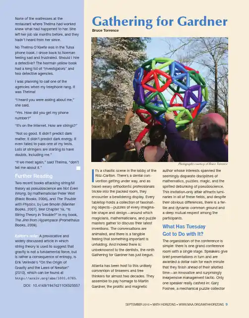
None of the waitresses at therestaurant where Thelma had worked knew what had happened to her. She left her job six months before, and they hadn’t heard from her since.No Thelma O’Keefe was in the Tulsa phone book. I drove back to Norman feeling sad and frustrated. Should I hire a detective? The Norman yellow book had a long list of “investigators” and two detective agencies.I was planning to call one of theagencies when my telephone rang. It was Thelma!“I heard you were asking about me,”she said.“Yes. How did you get my phone number?”“It’s on the Internet. How are strings?”“Not so good. It didn’t predict dark matter. It didn’t predict dark energy. It even failed to pass one of my tests.Lots of stringers are starting to have doubts, including me.”“If we meet again,” said Thelma, “don’t tell me about it.”Two recent books attacking string/M theory as pseudoscience are Not Even Wrong , by mathematician Peter Woit (Basic Books, 2006), and The Trouble with Physics , by Lee Smolin (Mariner Books, 2007). See Chapter 18, “Is String Theory in Trouble?” in my book,The Jinn from Hyperspace (Prometheus Books, 2008).A provocative and widely discussed article in which string theory is used to suggest that gravity is not a fundamental force, but is rather a consequence of entropy, is Erik Verlinde's “On the Origin of Gravity and the Laws of Newton”(2010), which can be found at/abs/1001.0785.DOI: 10.4169/194762110X525557Bruce TorrenceGathering for GardnerPhotographs courtesy of Bruce TorrenceIt’s a chaotic scene in the lobby of the Ritz-Carlton. There’s a dental con-vention getting under way, and as travel-weary orthodontic professionals trickle into the packed room, theyencounter a bewildering display. Every tabletop holds a collection of fascinat-ing objects—puzzles of every imagina-ble shape and design—around which magicians, mathematicians, and puzzle masters gather to discuss their latest inventions. The conversations are animated, and there is a tangible feeling that something important is unfolding. And indeed there is:unbeknownst to the dentists, the ninth Gathering for Gardner has just begun.Atlanta has been host to this unlikely convention of tinkerers and freethinkers for almost two decades. They assemble to pay homage to Martin Gardner, the prolific and magneticauthor whose interests spanned the seemingly disparate disciplines of mathematics, puzzles, magic, and the spirited debunking of pseudoscience.This invitation-only affair attracts lumi-naries in all of these fields, and despite their obvious differences, there is a fer-tile and dynamic common ground and a deep mutual respect among the participants.What Has Tuesday Got to Do with It?The organization of the conference is simple: there is one grand conference room with a single stage. Speakers give brief presentations in turn and are awarded a dollar coin for each minute that they finish ahead of their allotted time—an innovative and surprisingly inexpensive management tactic. Only one speaker really cashed in: Gary Foshee, a mechanical puzzle collectorthe week and that births are independ-ent of one another. With these assump-tions in hand, the puzzle succumbs easily to elementary probability theory.If one denotes a single birth by a two-tuple such as (boy, Tuesday) or (girl,Sunday), then there are 14 equally likely scenarios for a single birth. Foshee has two children, and with no other infor-mation, it follows that there are 142=196 equally likely poss bilities for two children. But at least one of his children is a (boy, Tuesday), and some simple counting reveals that just 27 of the 196outcomes satisfy this criterion. To see this, simply note that there are 14cases where the Tuesday boy is the first born, and 14 where he is the sec-ond born, and subtract the single case that was counted twice. Among these 27 equally likely poss bilities, how many include two boys? Exactly 13—there are seven with (boy, Tuesday) as the first child, and seven with (boy, Tues-day) as the second child, from which we subtract the one we counted twice.Hence, the answer to Foshee’s riddle is 13/27, close to, but not exactly, 1/2.Of course, the riddle leads naturally to a host of other questions. Does “one is a boy born on a Tuesday” mean that the other was not born on a Tuesday? I don’t read it this way. After all, the question makes clear that there is a poss bility that the second child is a boy, so why shouldn’t the child be allowed to arrive on a Tuesday also?More glaring is the counterintuitive nature of the result itself. Why should something like the day of the week affect the outcome? In thinking about this, it’s important to understand that had the day of the week not been mentioned, the answer would be 1/3,not 1/2, for only one of the threeequally likely gender scenarios BB, BG,GB yields two boys. It’s all aboutcounting the possible outcomes. If you are still wondering what Tuesday has to do with it, you may wish to consult the Further Reading section at the end ofthe article.illusion and perception, and on and on.The topics bounced so completely from one idea to the next that the effect was both intoxicating and refreshing. Spon-taneous discussion arose in and out of the conference room. “What does Tuesday have to do with it?”Foshee’s puzzle proved a perfect catalyst for discussion, and it is both fun and instructive to reason through it.One first has to make a few assump-tions, and most of the people I spoke with agreed that it’s best to keep it simple. Let’s assume that there are no multiple births, and that any single birth is equally likely to be a boy or a girl.Assume further that births are uniformlydistributed among the seven days ofand designer, faced the audience and spoke slowly, “I have two children. One is a boy born on a Tuesday. What is the probability I have two boys?” After a pause, he continued. “The first thing you think is ‘What has Tuesday got to do with it?’ Well, it has everything to do with it.” And with that, he stepped down (and collected a hefty stack of coins from the organizers).Other talks focused on space-filling curves and genome folding, origami mazes, Lewis Carroll’s mathematics,dancing tessellations, psychological explanations for children’s magictheory, the history of Rubik’s cube, the relation between computer hacking and invention, self-replicating machines,Just as Foshee’s riddle yields to elementary probability theory, the vast majority of questions and puzzles posed at the gathering can beapproached using basic principles.Each question has some clever twist,and of course this is the hallmark of a good brainteaser. Not all yield so easily,however. Bill Gosper, discoverer of the “glider gun” in Conway’s game of life and considered by many to be the founder of the hacker community,proudly shared his “Dozenegger”puzzle. This is a physical puzzle in which twelve circles, each a different size meticulously laser-cut from a sheet of acrylic, must be snuggly packed (but not forced) into a larger elliptical cavity.(You can find it on his website—see the Further Reading section.)Magic and illusion played a big part in the proceedings. Individual presenta-tions in this area fell squarely in the field of cognitive psychology, highlighting peculiarities in human perception. A cube with a corner removed can be interpreted at least three ways (a large cube with a smaller cube cut out of it; a large cube with a smaller cube jutting out from it; and a large three-sided “room” with a cube sitting in its back corner). Verses of Led Zepplin’s “Stairway to Heaven,” playedbackwards can be made to say pretty much whatever you want provided thelistener reads those words as it plays.Cinematic scenes in which actors changed costumes out of frame and returned in their new garb wentunnoticed by the entire audience (until we were prompted to look for the change in a second showing).Performance artists and magicians also took to the stage and presented stunning illusions with amazing skill.Attendees were treated to close-up magic after hours by some of the best in the business. The net effect was one of fascination with a subtly disturbing aftertaste. Everyone came away with a similar feeling: how is it that we can be deceived so easily? Seeing andbelieving will never again be the same.Abstract StructuresAnother highlight of the gathering was an afternoon dedicated to socializing and sculpture building. Attendees were invited to participate in the construction and installation of several mathematical sculptures at the home of TomRodgers, one of the main organizers of the event. On the lighter side, literally,Vi Hart led a group that created geometric balloon art. At the other extreme, Chaim Goodman-Strauss collaborated on a weighty steelsculpture that suggested a space-filling curve packed neatly into a cube. Other sculptures were created using materials such as aluminum, wood, bamboo, and plastic. Under the direction of their designers—George Hart, Carlo Séquin,Akio Hizume, Rinus Roelofs, among others—it was a tour de force of master craftsmen at the top of their game. The collaborative enterprise alsoemphasized to the pure mathemati-cians among us some of the practical difficulties that arise when an abstract idea is realized as a solid structure.Every sculpture presented unique challenges, and their successful resolution led to a deep sense offulfillment as the day came to a close.Back in the grand conference room, the onslaught of ideas continued. Princeton mathematician John H. Conway gave a spirited presentation on the arithmeticof lexicographic codes, or lexicodes as he calls them. Pure mathematics par excellence! Later,Scott Morris and Bruce Oberg gave back-to-back presentations heralding and bemoaning, respectively, the number nine (this being the ninth Gathering forGardner). Pure nonsense, with a nod toGardner’s fictitious numerologist and polymath, Dr. Matrix.As the barrage of topics flowed from the podium, what at first seemed a disparate hodgepodge of individually fascinating ideas began to gel into a coherent form. There was mathematics,there were puzzles, there was sleight of hand and deception, and there was mathematical artwork—the realization of abstract ideas into concrete form.There is beauty in all these, of course.But together the topics celebrate noth-ing less than our capacity to reason,and they demonstrate the supremacy of that endeavor. It is reason, after all,that enables us to solve mathematical problems and puzzles, and it is reason that enables us to test our often flawed perceptions and arrive at the truth.Collectively, the topics also payhomage to Martin Gardner himself, as they are precisely the themes that arose again and again in his writing. In the end, it is deeply inspiring to witness the extent to which his legacy lives on.Further ReadingFor more on Foshee’s Tuesday birthday problem, see Andrew Gelman’sStatistical Modeling, Causal Inference,and Social Science blog entry for May 27, 2010, titled “Hype about conditional probability puzzles” at/~co ok/movabletype/archives/2010/05/hype about cond.html .To feel the sting of Bill Gosper’s twelve-circle problem, download a (free) playable computer version of the puzzle athttp://demonstrations.wolfram.co m/TheTroublesomeTwelveCircleProb lem/.View the “Dozenegger” at/Dozenegger3.pdf .To test your skill at spotting a sleight of hand, check out “The Color-Changing Card Trick” at/watch?v=v oAntzB7EwE .The Ambiguous Corner Cube was first discussed in C. L. Strong’s “The Amateur Scientist” column in the November 1974 issue of Scientific American , p. 126. A template forconstructing a physical model can be found at/lite/inkjet science/pdfs/ProjectLITECornerCu beThirdCut.pdf .A brief introduction to Conway’s lexicode theorem is available at/semin ars/Kuwait/abstracts/L25.pdf ,and a more complete treatment can befound in MASS Selecta: Teaching and Learning Advanced Undergraduate Mathematics , edited by S. Katok, A.Sossinsky, and S. Tabachnikov (AMS,2003).For an introduction to the mysterious Dr. Matrix, see Martin Gardner’s The Magic Numbers of Dr. Matrix(Promethius Books, 1985). You might also enjoy the “Ask Dr. Matrix” online tool athttp://www.iread.it/ask matrix.php .DOI: 10.4169/194762110X525593About the author:Bruce Torrence is the Garnett Professor of Mathematics at Randolph-Macon College,and a co-editor of Math Horizons .email:****************。

a r X i v :a s t r o -p h /9901140v 1 12 J a n 1999Mon.Not.R.Astron.Soc.000,1–8(1998)Printed 1February 2008(MN L A T E X style file v1.4)UBV I CCD photometry of two old open clusters NGC 1798and NGC 2192Hong Soo Park and Myung Gyoon Lee ⋆Department of Astronomy,Seoul National University,Seoul 151-742,KoreaAccepted 1998??.Received 1998??;in original form 1998July ??ABSTRACT We present UBV I CCD photometry of two open clusters NGC 1798and NGC 2192which were little studied before.Color-magnitude diagrams of these clusters show several features typical for old open clusters:a well-defined main-sequence,a red giant clump,and a small number of red giants.The main sequence of NGC 1798shows a distinct gap at V ≈16.2mag.From the surface number density distribution we have measured the size of the clusters,obtaining 8′.3(=10.2pc)for NGC 1798and 7′.3(=7.5pc)for NGC 2192.Then we have determined the reddening,metallicity,and distance of these clusters using the color-color diagrams and color-magnitude diagrams:E (B −V )=0.51±0.04,[Fe/H]=−0.47±0.15dex and (m −M )0=13.1±0.2(d =4.2±0.3kpc)for NGC 1798,and E (B −V )=0.20±0.03,[Fe/H]=−0.31±0.15dex and (m −M )0=12.7±0.2(d =3.5±0.3kpc)for NGC 2192.The ages of these clusters have been estimated using the morphological age indicators and the isochrone fitting with the Padova isochrones:1.4±0.2Gyrs for NGC 1798and 1.1±0.1Gyrs for NGC 2192.The luminosity functions of the main sequence stars in these clusters are found to be similar to other old open clusters.The metallicity and distance of these clusters are consistent with the relation between the metallicity and galactocentric distance of other old open clusters.Key words:Hertzsprung–Russell (HR)diagram –open clusters and associations:general –open clusters and associations:individual:NGC 1798,NGC 2192–stars:luminosity function.1INTRODUCTIONOld open clusters provide us with an important informationfor understanding the early evolution of the Galactic disk.There are about 70known old open clusters with age >1Gyrs (Friel 1995).These clusters are faint in general so thatthere were few studies about these clusters until recently.With the advent of CCD camera in astronomy,the numberof studies on these clusters has been increasing.However,there are still a significant number of old open clusters forwhich basic parameters are not well known.For example,metallicity is not yet known for about 30clusters amongthem.Recently Phelps et al.(1994)and Janes &Phelps (1994)presented an extensive CCD photometric survey of potentialold open clusters,the results of which were used in the studyon the development of the Galactic disk by Janes &Phelps(1994).In the sample of the clusters studied by Phelps et al.⋆corresponding author,E-mail:mglee@astrog.snu.ac.krthere are several clusters for which only the non-calibrated photometry is available.We have chosen two clusters among them,NGC 1798and NGC 2192,to study the characteristics of these clus-ters using UBV I CCD photometry.These clusters are lo-cated in the direction of anti-galactic centre.To date there is published only one photometric study of these clusters,which was given by Phelps et al.(1994)who presented non-calibrated BV CCD photometry of these clusters.From the instrumental color-magnitude diagrams of these clus-ters Phelps et al.estimated the ages of these clusters using the morphological age indicators,obtaining the values of 1.5Gyrs for NGC 1798and 1.1Gyrs for NGC 2192.However,no other properties of these clusters are yet known.In this paper we present a study of NGC 1798and NGC 2192based on UBV I CCD photometry.We have es-timated the basic parameters of these clusters:size,red-dening,metallicity,distance,and age.Also we have derived the luminosity function of the main sequence stars in these clusters.Section 2describes the observations and data re-duction.Sections 3and 4present the analysis for NGC 1798c 1998RAS2Hong Soo Park and Myung Gyoon Leeand NGC2192,respectively.Section5discusses the results. Finally Section6summarizes the primary results.2OBSER V ATIONS AND DATA REDUCTION 2.1ObservationsUBV I CCD images of NGC1798and NGC2192were obtained using the Photometrics512CCD camera at the Sobaeksan Observatory61cm telescope in Korea for several observing runs between1996November and1997October. We have used also BV CCD images of the central region of NGC1798obtained by Chul Hee Kim using the Tek1024 CCD camera at the Vainu Bappu Observatory2.3m tele-scope in India on March4,1998.The observing log is given in Table1.The original CCD images wereflattened after bias sub-traction and several exposures for eachfilter were combined into a single image for further reduction.The sizes of the field in a CCD image are4′.3×4′.3for the PM512CCD im-age,and10′.6×10′.6for the Tek1024CCD image.The gain and readout noise are,respectively,9electrons/ADU and 10.4electrons for the PM512CCD,and9electrons/ADU and10.4electrons for the Tek1024CCD.Figs.1and2illustrate grey scale maps of the V CCD images of NGC1798and NGC2192made by mosaicing the images of the observed regions.It is seen from thesefigures that NGC1798is a relatively rich open cluster,while NGC 2192is a relatively poor open cluster.2.2Data ReductionInstrumental magnitudes of the stars in the CCD images were obtained using the digital stellar photometry reduction program IRAF⋆/DAOPHOT(Stetson1987,Davis1994). The resulting instrumental magnitudes were transformed onto the standard system using the standard stars from Lan-dolt(1992)and the M67stars in Montgomery et al.(1993) observed on the same photometric nights.The transforma-tion equations areV=v+a V(b−v)+k V X+Z V,(B−V)=a BV(b−v)+k BV X+Z BV,(U−B)=a UB(u−b)+k UB X+Z UB,and(V−I)=a V I(v−i)+k V I X+Z V I,where the lower case symbols represent instrumental mag-nitudes derived from the CCD images and the upper case symbols represent the standard system values.X is the air-mass at the midpoint of the observations.The results of the transformation are summarized in Table2.The data ob-tained on non-photometric nights were calibrated using the photometric data for the overlapped region.The total number of the measured stars is1,416for NGC1798and409for NGC2192.Tables3and4list the⋆IRAF is distributed by the National Optical Astronomy Ob-servatories,which are operated by the Association of Universities for Research in Astronomy,Inc.under contract with the National Science Foundation.photometry of the bright stars in the C-regions of NGC1798 and NGC2192,respectively.The X and Y coordinates listed in Table3and4are given in units of CCD pixel(=0′′.50). The X and Y values are increasing toward north and west, respectively.We have divided the entire region of thefields into sev-eral regions,as shown in Figs.1and2,for the analysis of the data.The C-region represents the central region of the cluster,and the F-regions(F,Fb,Fir,and Fi regions)rep-resent the controlfield regions,and the N-region represents the intermediate region between the central region and the field region.The radius of the C-region is300pixel for NGC 1798and NGC2192.The ratio of the areas of the C-region, N-region,Fb-region,and(Fi+Fir)-regions for NGC1798is 1:1.50:1.00:1.07,and the ratio of the areas of the C-region, N-region,and F-region for NGC2192is1:1.26:0.98.3ANALYSIS FOR NGC17983.1The Size of the ClusterWe have investigated the structure of NGC1798using star-counts.The centre of the cluster is estimated to be at the po-sition of(X=710pixel,Y=1110pixel),using the centroid method.Fig.3illustrates the projected surface number den-sity profile derived from counting stars with V<19.5mag in the entire CCDfield.The magnitude cutofffor starcounts was set so that the counts should be free of any photometric incompleteness problem.Fig.3shows that most of the stars in NGC1798are concentrated within the radius of250pixel (=125′′),and that the outskirts of the cluster extend out to about500pixel(=250′′)from the center.The number density changes little with radius beyond500pixel,show-ing that the outer region of the observedfield can be used as a controlfield.Therefore we have estimated the approxi-mate size of NGC1798for which the cluster blends in with thefield to be about500′′in diameter,which corresponds to a linear size of10.2pc for the distance of NGC1798as determined below.3.2Color-Magnitude DiagramsFigs.4and5show the V−(B−V)and V−(V−I)color-magnitude diagrams(CMDs)of the measured stars in the observed regions in NGC1798.Thesefigures show that the C-region consists mostly of the members of NGC1798with some contamination of thefield stars,while the F-regions consist mostly of thefield stars.The N-region is intermediate between the C-region and the F-region.The distinguishable features seen in the color-magnitude diagrams of the C-region are:(a)There is a well-defined main sequence the top of which is located at V≈16 mag;(b)There is seen a distinct gap at V≈16.2mag in the main sequence,which is often seen in other old open clusters (e.g.M67);(c)There is a poorly defined red giant branch and these is seen some excess of stars around(B−V)=1.3 and V=15.6mag on this giant branch,which is remarked by the small box in thefigures.This may be a random excess of stars.However,the positions of the stars in the CMDs are consistent with the positions of known red giant clump in other old open clusters.Therefore most of these stars arec 1998RAS,MNRAS000,1–8UBV I CCD photometry of two old open clusters NGC1798and NGC21923probably red giant clump stars;and(d)There are a small number of stars along the locus of the red giant branch. 3.3Reddening and MetallicityNGC1798is located close to the galactic plane in the anti-galactic centre direction(b=4◦.85and l=160◦.76)so that it is expected that the reddening toward this cluster is significant.We have estimated the reddening for NGC1798 using two methods as follows.First we have used the mean color of the red giant clump.Janes&Phelps(1994)estimated the mean color and magnitude of the red giant clump in old open clusters to be (B−V)RGC=0.87±0.02and M V,RGC=0.59±0.09,when the difference between the red giant clump and the main sequence turn-offof the clusters,δV,is smaller than one. The mean color of the red giant clump in the C-region is estimated to be(B−V)RGC=1.34±0.01((V−I)RGC= 1.47±0.01,and(U−B)RGC=1.62±0.04),and the cor-responding mean magnitude is V RGC=15.57±0.05.δV is estimated to be0.8±0.2,which is the same value derived by Phelps et al.(1994).From these data we have derived a value of the reddening,E(B−V)=0.47±0.02.Secondly we have used the color-color diagram to es-timate the reddening and the metallicity simultaneously. We havefitted the mean colors of the stars in the C-region with the color-color relation used in the Padova isochrones (Bertelli et al.1994).This process requires iteration,because we need to know the age of the cluster as well as the red-dening and metallicity.We have iterated this process until all three parameters are stabilized.Fig.6illustrates the results offitting in the(U−B)−(B−V)color-color diagram.It is shown in thisfigure that the stars in NGC1798are reasonablyfitted by the color-color relation of the isochrones for[Fe/H]=−0.47±0.15 with a reddening value of E(B−V)=0.55±0.05. The error for the metallicity,0.15,was estimated by com-paring isochrones with different metallicities.As a reference the mean locus of the giants for solar abundance given by Schmidt-Kaler(1982)is also plotted in Fig.6.Finally we derive a mean value of the two estimates for the reddening, E(B−V)=0.51±0.04.3.4DistanceWe have estimated the distance to NGC1798using two methods as follows.First we have used the mean magnitude of the red giant clump.We have derived a value of the ap-parent distance modulus(m−M)V=14.98±0.10from the values for the mean magnitudes of the red giant clump stars described above.Secondly we have used the the zero-age main sequence (ZAMS)fitting,following the method described in Vanden-Berg&Poll(1989).VandenBerg&Poll(1989)presented the semi-empirical ZAMS as a function of the metallicity[Fe/H] and the helium abundance Y:V=M V(B−V)+δM V(Y)+δM V([Fe/H])whereδM V(Y)=2.6(Y−0.27)andδM V([Fe/H])=−[Fe/H](1.444+0.362[Fe/H]).Before the ZAMSfitting,we subtracted statistically the contribution due to thefield stars in the CMDs of the C-region using the CMDs of the Fb-region for BV photometry and the CMDs of the Fi+Fir region for V I photometry. The size of the bin used for the subtraction is∆V=0.25 and∆(B−V)=0.1.The resulting CMDs are displayed in Fig.7.We used the metallicity of[Fe/H]=–0.47as derived above and adopted Y=0.28which is the mean value for old open clusters(Gratton1982).Using this method we have obtained a value of the apparent distance modulus(m−M)V=14.5±0.2.Finally we calculate a mean value of the two estimates,(m−M)V=14.7±0.2.Adopting the extinction law of A V=3.2E(B−V),we derive a value of the intrinsic distance modulus(m−M)0=13.1±0.2.This corresponds to a distance of d=4.2±0.3kpc.3.5AgeWe have estimated the age of NGC1798using two methods as follows.First we have used the morphological age index (MAI)as described in Phelps et al.(1994).Phelps et al. (1994)and Janes&Phelps(1994)presented the MAI–δV relation,MAI[Gyrs]=0.73×10(0.256δV+0.0662δV2).From the value ofδV derived above,0.8±0.2mag,we obtain a value for the age,MAI=1.3±0.2Gyrs.Secondly we have estimated the age of the cluster us-ing the theoretical isochrones given by the Padova group (Bertelli et al.1994).Fitting the isochrones for[Fe/H]=–0.47to the CMDs of NGC1798,as shown in Fig.8,we estimate the age to be1.4±0.2Gyrs.Both results agree very well.3.6Luminosity FunctionWe have derived the V luminosity functions of the main sequence stars in NGC1798,which are displayed in Fig.9.The Fb-region was used for subtraction of thefield star contribution from the C-region and the magnitude bin size used is0.5mag.This controlfield may not be far enough from the cluster to derive thefield star contribution.If so,we might have oversubtracted thefield contribution,obtaining flatter luminosity functions than true luminosity functions. However,the fraction of the cluster members in thisfield must be,if any,very low,because the surface number density of this region is almost constant with the radius as shown in Fig.3.The luminosity function of the C-region in Fig. 9(a)increases rapidly up to V≈16.5mag,and stays almost flat for V>16.5mag.The luminosity functions of the N-region and the(R+Fir)-region are steeper than that of the C-region.A remarkable drop is seen at V=16.2mag(M V= 1.5mag)in the luminosity function of the C-region based on smaller bin size of0.2mag in Fig.9(b).This corresponds to the main sequence gap described above.4ANALYSIS FOR NGC21924.1The Size of the ClusterWe have investigated the structure of NGC2192using star-counts.We could not use the centroid method to estimatec 1998RAS,MNRAS000,1–84Hong Soo Park and Myung Gyoon Leethe centre of this cluster,because this cluster is too sparse. So we have used eye-estimate to determine the centre of the cluster to be at the position of(X=465pixel,Y=930 pixel).Fig.10illustrates the projected surface number den-sity profile derived from counting stars with V<18mag in the entire CCDfield.The magnitude cutofffor starcounts was set so that the counts should be free of any photomet-ric incompleteness problem.Fig.10shows that most of the stars in NGC2192are concentrated within the radius of200 pixel(=100′′),and that the outskirts of the cluster extend out to about440pixel(=220′′)from the centre.Therefore the approximate size of NGC2192is estimated to be about 440′′in diameter,which corresponds to a linear size of7.5pc for the distance of NGC2192as determined below.4.2Color-Magnitude DiagramsFigs.11and12show the V−(B−V)and V−(V−I)color-magnitude diagrams of the measured stars in the observed regions in NGC2192.The distinguishable features seen in the color-magnitude diagrams of the C-region are:(a)There is a well-defined main sequence the top of which is located at V≈14mag;(b)There are a group of red giant clump stars at(B−V)=1.1and V=14.2mag,which are remarked by the small box in thefigures;and(c)There are a small number of stars along the locus of the red giant branch. 4.3Reddening and MetallicityNGC2192is located11degrees above the galactic plane in the anti-galactic centre direction(b=10◦.64and l= 173◦.41)but higher than NGC1798so that it is expected that the reddening toward this cluster is significant but smaller than that of NGC1798.We have estimated the red-dening for NGC2192using two methods as applied for NGC 1798.First we have used the mean color of the red giant clump.The mean color of the red giant clump in the C-region is estimated to be(B−V)RGC=1.08±0.01((V−I)RGC=1.07±0.01,and(U−B)RGC=0.61±0.02),and the corresponding mean magnitude is V RGC=14.20±0.05.δV is estimated to be0.6±0.2,which is similar to the value derived by Phelps et al.(1994).From these data we have derived a value of the reddening,E(B−V)=0.19±0.03.Secondly we have used the color-color diagram to es-timate the reddening and the metallicity simultaneously. We havefitted the mean colors of the stars in the C-region with the color-color relation used in the Padova isochrones (Bertelli et al.1994).Fig.13illustrates the results offit-ting in the(U−B)−(B−V)color-color diagram.It is shown in thisfigure that the stars in NGC2192are rea-sonablyfitted by the color-color relation of the isochrones for[Fe/H]=−0.31±0.15dex with a reddening value of E(B−V)=0.21±0.01.The error for the metallicity,0.15, was estimated by comparing isochrones with different metal-licities.As a reference the mean locus of the giant for solar abundance given by Schmidt-Kaler is also plotted in Fig.13. Finally we derive a mean value of the two estimates for the reddening,E(B−V)=0.20±0.03.4.4DistanceWe have estimated the distance to NGC2192using two methods as for NGC1798.First we have used the mean magnitude of the red giant clump.We have derived a value of the apparent distance modulus(m−M)V=13.61±0.10 from the values for the mean magnitudes of the red giant clump stars described previously.Secondly we have used the ZAMSfitting.Before the ZAMSfitting,we subtracted statistically the contribution due to thefield stars in the CMDs of the C-region using the CMDs of the F-region.The size of the bin used for the subtraction is∆V=0.25and∆(B−V)=0.1.The resulting CMDs are displayed in Fig.14.We used the metallicity of[Fe/H]=–0.31as derived before and adopted Y=ing this method we have obtaineda value of the apparent distance modulus(m−M)V=13.1±0.2.Finally we calculate a mean value of the two estimates,(m−M)V=13.3±0.2.Adopting the extinction law of A V=3.2E(B−V),we derive a value of the intrinsic distance modulus(m−M)0=12.7±0.2.This corresponds to a distance of d=3.5±0.3kpc.4.5AgeWe have estimated the age of NGC2192using two methods as follows.First we have used the morphological age index. From the value ofδV derived above,0.6±0.2mag,we obtain a value for the age,MAI=1.1±0.2Gyrs.Secondly we have estimated the age of the cluster using the theoretical isochrones given by the Padova group(Bertelli et al.1994). Fitting the isochrones for[Fe/H]=–0.31to the CMDs of NGC2192,as shown in Fig.15,we estimate the age to be 1.1±0.1Gyrs.Both results agree very well.4.6Luminosity FunctionWe have derived the V luminosity functions of the main sequence stars in NGC2192,which are displayed in Fig.16.The F-region was used for subtraction of thefield star contribution from the C-region.The luminosity function of the C-region in Fig.16(a)increases rapidly up to V≈14 mag,and stays almostflat for V>15mag.The luminosity function of the N-region is steeper than that of the C-region. Fig.16(b)displays a comparison of the luminosity functions of NGC1798,NGC2192,and NGC7789which is another old open cluster of similar age(Roger et al.1994).Fig.16(b) shows that the luminosity functions of these clusters are similar in that they are almostflat in the faint part.The flattening of the faint part of the luminosity functions of old open clusters has been known since long,and is believed to be due to evaporation of low mass stars(Friel1995).5DISCUSSIONWe have determined the metallicity and distance of NGC 1798and NGC2192in this study.We compare them with those of other old open clusters here.Fig.17illustrates the radial metallicity gradient of the old open clusters com-piled by Friel(1995)and supplemented by the data in Wee&Lee(1996)and Lee(1997).Fig.17shows that thec 1998RAS,MNRAS000,1–8UBV I CCD photometry of two old open clusters NGC1798and NGC21925 mean metallicity decreases as the galactocentric distance in-creases.The positions of NGC1798and NGC2192we haveobtained in this study are consistent with the mean trendof the other old open clusters.The slope we have deter-mined for the entire sample including these two clusters is∆[Fe/H]/R GC=−0.086±0.011dex/kpc,very similar tothat given in Friel(1995),∆[Fe/H]/R GC=−0.091±0.014dex/kpc.There are only four old open clusters located beyondR GC=13kpc in Fig.17.These four clusters follow the meantrend of decreasing outward.However,the number of theclusters is not large enough to decide whether the metallictykeeps decreasing outward or it stops decreasing somewherebeyond R GC=13kpc and stays constant.Further studiesof more old open clusters beyond R GC=13kpc are neededto investigate this point.6SUMMARY AND CONCLUSIONSWe have presented UBV I photometry of old open clustersNGC1798and NGC2192.From the photometric data wehave determined the size,reddening,metallicity,distance,and age of these clusters.The luminosity functions of themain sequence stars in these clusters are similar to those ofthe other old open clusters.The basic properties of theseclusters we have determined in this study are summarizedin Table5.ACKNOWLEDGMENTSProf.Chul Hee Kim is thanked for providing the BV CCDimages of NGC1798.This research is supported in part bythe Korea Science and Engineering Foundation Grant No.95-0702-01-01-3.REFERENCESBertelli,G.,Bressan,A.,Chiosi,C.,Fagotto,F.,&Nasi,E.1994,A&AS,106,275Davis,L.E.,1994,A Reference Guide to the IRAF/DAOPHOTPackageFriel,E.D.1995,ARA&A,33,381Gratton,R.G.,1982,ApJ,257,640Janes,K.,&Phelps,R.L.1994,AJ,108,1773Landolt,A.U.,1992,AJ,104,340Lee,M.G.,1997,113,729Montgomery,K.A.,Marschall,L.A.,&Janes,K.A.1993,AJ,106,181Phelps,R.L.,Janes,K.,&Montgomery,K.A.,1994,AJ,107,1079Roger,C.M.,Paez,E.,Castellani,V.,&Staniero,O.1994,A&A,290,62Schmidt-Kaler,T.1982,in Landolt-Bornstein VI,2b(Berlin:Springer)Stetson,P.B.,1987,PASP,99,191VandenBerg,D.A.,&Poll,H.E.,1989,AJ,98,1451Wee,S.O.,&Lee,M.G.,1996,Jour.Korean Astro.Soc.,29,181This paper has been produced using the Royal AstronomicalSociety/Blackwell Science L A T E X stylefile.c 1998RAS,MNRAS000,1–86Hong Soo Park and Myung Gyoon LeeTable2.Transformation coefficients for the standard stars.Date Color a k Z rms n(stars) 96.11.11V0.003–0.101–6.0400.00919(B−V) 1.090–0.155–0.4670.01317(U−B) 1.008–0.154–1.7110.03416 97.02.11V0.028–0.198–6.0500.00934(B−V) 1.150–0.118–0.5930.01035(U−B) 1.079–0.324–1.5750.03226(V−I)0.983–0.1300.3020.00829 97.02.13V–0.007–0.176–6.0050.01034(B−V) 1.160–0.133–0.5880.01334(U−B) 1.079–0.349–1.5260.02320(V−I)0.986–0.0970.2710.01532 97.03.17V-0.019–0.225–6.0680.01548(B−V) 1.221–0.093–0.7810.01844(U−B) 1.008–0.309–1.4580.02735(V−I)0.956–0.1570.3140.02052Table 3.UBV I photometry of the bright stars in the C-regionof NGC1798.ID X[px]Y[px]V(B−V)(U−B)(V−I) 1723.21110.815.8600.7790.3240.9143680.51092.015.380 1.3250.627 1.5254746.01160.315.9050.7410.2200.9545741.81165.514.380 1.4830.880 1.6336684.61030.115.8140.8640.342 1.0427745.31073.315.3760.9200.237 1.0849707.21038.814.777 1.4860.723 1.653 11549.41153.715.305 1.5290.915 1.666 12547.91162.714.846 1.6270.947 1.764 13602.31068.015.325 1.5240.847 1.660 14598.11080.815.776 1.3340.575 1.490 15525.81116.815.510 1.0020.346 1.169 18833.91144.214.976 1.4940.866 1.578 21981.91125.114.711 1.510 1.031 1.440 26835.71098.015.706 1.3180.468 1.407 27656.51022.115.653 1.4160.180 1.571 28659.8955.915.216 1.2160.384 1.385 29656.4976.813.6670.6610.3100.777 30674.2822.512.0330.4450.0500.532 33668.7966.315.687 1.3130.641 1.446 34764.3879.915.460 1.3370.508 1.408 38749.01008.115.359 1.3220.744 1.426 39774.4965.915.545 1.3040.590 1.402 43571.8930.612.875 1.970 1.264 2.252 45512.8908.715.810 1.3480.474 1.485 46642.1949.515.622 1.3290.590 1.477 48732.61211.315.821 1.3530.643 1.492 50678.81210.515.297 1.3680.770 1.501 51742.11244.414.7990.747-0.046 1.216 52673.11250.215.180 1.3060.780 1.457 56728.21183.415.665 1.4050.803 1.545 57614.91229.413.085 2.1770.635 3.581 62563.01338.415.9090.7060.6380.778 65913.91203.013.686 1.2490.851 1.354 67792.71314.215.6010.9750.470 1.275 68932.61268.414.4660.7170.1970.763 70801.11338.715.561 1.3270.785 1.442 72827.61315.513.5260.9670.521 1.161 78444.01094.814.605 1.5790.825 1.723 82684.3822.615.8280.9510.128 1.189 97598.51330.315.580 1.3360.710 1.483Table4.UBV I photometry of the bright stars in the C-region of NGC2192.ID X[px]Y[px]V(B−V)(U−B)(V−I) 4502.4879.614.9830.4320.1140.424 5537.5891.712.9690.9240.4750.930 7535.1931.315.1700.598-0.2010.483 9434.8947.613.6760.570-0.0560.648 10562.3991.914.037 1.0960.612 1.043 11412.9884.814.165 1.0780.608 1.072 12598.4778.715.1840.464-0.0300.477 13595.9930.014.4800.5020.1720.549 14625.8971.814.7430.7200.0890.741 16614.3684.214.3970.7660.1750.758 17463.3689.514.7660.4660.0120.480 18553.3710.715.4920.447-0.1350.428 19591.7723.814.4660.5450.0930.566 21623.0867.712.634 1.1020.713 1.108 22648.0929.015.3380.3940.1150.399 26461.1711.314.162 1.0860.670 1.091 29583.9802.315.0940.600-0.0160.644 32720.4889.515.3260.3700.0710.410 37395.9778.315.2640.3960.0310.379 38405.5778.514.8900.4810.1010.409 40258.21042.915.4310.4240.1200.484 42376.6883.915.1870.4550.1360.470 44180.1908.714.3200.2870.1120.295 47367.1938.314.8970.4030.2520.459 51183.3998.714.202 1.1140.552 1.108 55475.81052.514.6370.3880.1670.465 56389.11055.113.6060.6520.2560.777 58481.41074.114.3470.4500.1150.520 59514.91085.115.0970.4290.1370.517 60478.51089.614.2360.5280.1590.582 61498.51127.914.6090.5090.1350.578 63278.71154.414.372 1.0700.599 1.053 64527.41158.715.4180.4460.2450.510 65343.41167.814.266 1.0120.618 1.035 66362.21169.314.2660.8790.4690.879 74346.91039.814.5810.4520.1240.510 77688.91124.215.4200.3900.2900.400 83678.91079.715.4950.4640.1070.504 84624.21042.813.5010.3850.2170.389 88579.61028.914.8250.4560.1620.530 Table5.Basic properties of NGC1798and NGC2192.Parameter NGC1798NGC2192RA(2000)5h11m40s6h15m11sDEC(2000)47◦40′37′′39◦51′1′′l160◦.76173◦.41b4◦.8510◦.64Age1.4±0.2Gyrs1.1±0.1GyrsE(B−V)0.51±0.040.20±0.04[Fe/H]−0.47±0.15dex−0.31±0.15dex(m−M)013.1±0.212.7±0.2distance4.2±0.3kpc3.5±0.3kpcR GC12.5kpc11.9kpcz355pc646pcdiameter10.2pc(8′.3)7.5pc(7′.3)c 1998RAS,MNRAS000,1–8UBV I CCD photometry of two old open clusters NGC1798and NGC21927 Table1.Observing log for NGC1798and NGC2192.Date Target Filter Seeing Telescope Condition96.11.11NCC1798UBV2′′.3SAO a-61cm Photometric97.01.12NCC1798UBV I2′′.2SAO-61cm Non-photometric97.02.12NCC1798,NGC2192UBV I3′′.3SAO-61cm Photometric97.02.13NCC1798,NGC2192UBV I2′′.5SAO-61cm Non-photometric97.03.17NCC2192UBV I2′′.2SAO-61cm Photometric97.10.21NCC1798BV I2′′.3SAO-61cm Non-photometric97.10.24NCC2192BV I2′′.7SAO-61cm Non-photometric97.03.04NCC1798BV2′′.7VBO b-2.3m Non-photometrica Sobaeksan Astronomical Observatoryb Vainu Bappu Observatoryc 1998RAS,MNRAS000,1–8。