概率论英文版第二章
- 格式:doc
- 大小:1.78 MB
- 文档页数:14

普林斯顿的概率论英文版I believe that the English version of the probability theory book by Princeton University Press is a valuable resource for students and researchers in the field of mathematics and statistics. This book provides a comprehensive and rigorous treatment of probability theory, covering key concepts and techniques essential for understanding and analyzing probabilistic phenomena.我相信普林斯顿大学出版社的概率论英文版是数学和统计学领域的学生和研究人员的宝贵资源。
这本书全面而严谨地讨论了概率论的关键概念和技术,涵盖了理解和分析概率现象所必不可少的内容。
The book starts with an introduction to the fundamental principles of probability, such as sample spaces, events, and probability measures. It then moves on to discuss random variables, probability distributions, and mathematical expectation, providing a solid foundation for more advanced topics in probability theory.这本书首先介绍了概率的基本原理,如样本空间、事件和概率测度。

概率论与数理统计课程教学大纲编辑整理:尊敬的读者朋友们:这里是精品文档编辑中心,本文档内容是由我和我的同事精心编辑整理后发布的,发布之前我们对文中内容进行仔细校对,但是难免会有疏漏的地方,但是任然希望(概率论与数理统计课程教学大纲)的内容能够给您的工作和学习带来便利。
同时也真诚的希望收到您的建议和反馈,这将是我们进步的源泉,前进的动力。
本文可编辑可修改,如果觉得对您有帮助请收藏以便随时查阅,最后祝您生活愉快业绩进步,以下为概率论与数理统计课程教学大纲的全部内容。
《概率论与数理统计》课程教学大纲(2002年制定 2004年修订)课程编号:英文名:Probability Theory and Mathematical Statistics课程类别:学科基础课前置课:高等数学后置课:计量经济学、抽样调查、试验设计、贝叶斯统计、非参数估计、统计分析软件、时间序列分析、统计预测与决策、多元统计分析、风险理论学分:5学分课时:85课时修读对象:统计学专业学生主讲教师:杨益民等选定教材:盛骤等,概率论与数理统计,北京:高等教育出版社,2001年(第三版)课程概述:本课程是统计学专业的学科基础课,是研究随机现象统计规律性的一门数学课程,其理论及方法与数学其它分支、相互交叉、渗透,已经成为许多自然科学学科、社会与经济科学学科、管理学科重要的理论工具。
由于其具有很强的应用性,特别是随着统计应用软件的普及和完善,使其应用面几乎涵盖了自然科学和社会科学的所有领域。
本课程是统计专业学生打开统计之门的一把金钥匙,也是经济类各专业研究生招生考试的重要专业基础课。
本课程由概率论与数理统计两部分组成。
概率论部分侧重于理论探讨,介绍概率论的基本概念,建立一系列定理和公式,寻求解决统计和随机过程问题的方法。
其中包括随机事件和概率、随机变量及其分布、随机变量的数字特征、大数定律和中心极限定理等内容;数理统计部分则是以概率论作为理论基础,研究如何对试验结果进行统计推断。
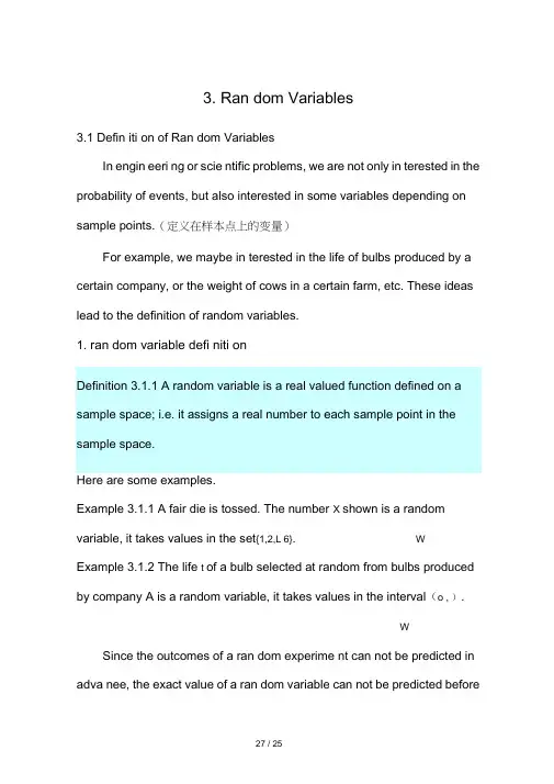
3. Ran dom Variables3.1 Defin iti on of Ran dom VariablesIn engin eeri ng or scie ntific problems, we are not only in terested in the probability of events, but also interested in some variables depending on sample points.(定义在样本点上的变量)For example, we maybe in terested in the life of bulbs produced by a certain company, or the weight of cows in a certain farm, etc. These ideas lead to the definition of random variables.1. ran dom variable defi niti onExample 3.1.1 A fair die is tossed. The number X shown is a random variable, it takes values in the set{1,2,L 6}. WExample 3.1.2 The life t of a bulb selected at random from bulbs produced by company A is a random variable, it takes values in the interval(o , ).W Since the outcomes of a ran dom experime nt can not be predicted in adva nee, the exact value of a ran dom variable can not be predicted beforethe experiment, we can only discuss the probability that it takes somevalue or the values in some subset of R.2. Distribution functionDefinition 3.1.2 Let X be a random variable on the sample space S. Then the fun cti onF(X) P(X x). x Ris called the distribution function of XNote The distribution function F(x)is defined on real numbers, not on sample space.Example 3.1.3 Let X be the number we get from tossing a fair die. Then the distribution function of X is (Figure 3.1.1)0, if x 1;nF (x) , if n x n 1,n 1,2,L ,5;61, if x 6.P11门3. Properties 1 2 3 4 5b "Figure 3.1.1 The distributio n fun cti on in ExampleThe distribution function F(x)of a random variable X has the followi ng properties:(1) F(x) is non-decreasing.In fact, if x 1 x 2, the n the eve nt {Xis a subset ofthe eve nt{X x 2} ,thusF(xJ P(XX 1)P(XX 2) F(X 2)⑵F()lim F(x)xo,F()Jim F(x)1.(3)For any x 0 R ,li mX x oF(x) F(x o0) F(x )) .This is to say, thedistribution function F (x )of a random variable X is right continuous. Example 3.1.4 Let X be the life of automotive parts produced by company A , assume the distribution function of X is (in hours)xF (x) P(X x) I II e 2000, x 0;0, x 0.Find P(X 2ooo ),p (1ooo X 3000).Question : What are the probabilities P(X 2000) and P(X 2000)Soluti onSoluti on By defi niti on,IIP(X 2000)F(2000)1 e 0.6321 .P(1000 X 3000) P(X 3000) P(X1000)F(1000)(1 e 1.5) (1 e 0.5)Let X1be the total number shown, then the events{ X1 k} contains k 1 sample points, k 234,5 . Thusk 1P(X1 k) , k 2,3,4,536And5{X 1} U{X1 k}k 2so5 5P(X 1) P(X k)k 218P(X 1) 1 P(X 1) 1 3 1Thus0, x 1;5F(x) P(X x) , 1 x 1;181, x 1.1. - •--------- oFigure 3.1.2 The distribution function in Example 3.1.5In this book, we study two kinds of ran dom variables.X X 佝忌丄a n 丄}. LetP(X a n ) P n ,n 1,2,L .(3.2.1)Then we have p n o , n 1,2,L , p n 1.nthe probability distributi on of the discrete ran dom variable X (概率分 布)注意随机变量X 的分布所满足的条件(1) P i > 0(2) P 1+P 2+…+P n =1离散型分布函数And the distribution function of X is given byF(x) P(X x) P n(3.2.2)an XFor an experime nt in which a coi n is tossed three times (or 3 coins are tossed on ce), con struct the distributi on ofX. (Let X denote the nu mber of head occurre nee)Soluti onn=3, p=1/2__pr0 1/81 3/82 3/83 1/8Example 2在一次试验中,事件A发生的概率为p,不发生的概率为1-p,用X=0表示事件A没有发生,X=1表示事件A发生,求X的分布。
概率论与数理统计Probability Theory and Mathematical Statistics第一章概率论的基本概念Chapter 1 Introduction of Probability Theory不确定性indeterminacy必然现象certain phenomenon随机现象random phenomenon试验experiment结果outcome频率数frequency number样本空间sample space出现次数frequency of occurrencen维样本空间n-dimensional sample space样本空间的点point in sample space随机事件random event / random occurrence基本事件elementary event必然事件certain event不可能事件impossible event等可能事件equally likely event事件运算律operational rules of events事件的包含implication of events并事件union events交事件intersection events互不相容事件、互斥事件mutually exclusive events / /incompatible events 互逆的mutually inverse加法定理addition theorem古典概率classical probability古典概率模型classical probabilistic model几何概率geometric probability乘法定理 product theorem概率乘法 multiplication of probabilities条件概率 conditional probability全概率公式、全概率定理 formula of total probability贝叶斯公式、逆概率公式 Bayes formula后验概率 posterior probability先验概率 prior probability独立事件 independent event独立随机事件 independent random event独立实验 independent experiment两两独立 pairwise independent两两独立事件 pairwise independent events第二章随机变量及其分布Chapter 2 Random V ariables and Distributions随机变量 random variables离散随机变量 discrete random variables概率分布律 law of probability distribution一维概率分布 one-dimension probability distribution概率分布 probability distribution两点分布 two-point distribution伯努利分布 Bernoulli distribution二项分布/伯努利分布 Binomial distribution超几何分布 hyper geometric distribution三项分布 trinomial distribution多项分布 polynomial distribution泊松分布 Poisson distribution泊松参数 Poisson theorem分布函数 distribution function概率分布函数 probability density function连续随机变量 continuous random variable概率密度 probability density概率密度函数 probability density function概率曲线 probability curve均匀分布 uniform distribution指数分布 exponential distribution指数分布密度函数 exponential distribution density function正态分布、高斯分布 normal distribution标准正态分布 standard normal distribution正态概率密度函数 normal probability density function正态概率曲线 normal probability curve标准正态曲线 standard normal curve柯西分布 Cauchy distribution分布密度 density of distribution第三章多维随机变量及其分布Chapter 3 Multivariate Random Variables and Distributions 二维随机变量 two-dimensional random variable联合分布函数 joint distribution function二维离散型随机变量 two-dimensional discrete random variable二维连续型随机变量 two-dimensional continuous random variable联合概率密度 joint probability variablen维随机变量 n-dimensional random variablen维分布函数 n-dimensional distribution functionn维概率分布 n-dimensional probability distribution边缘分布 marginal distribution边缘分布函数 marginal distribution function边缘分布律 law of marginal distribution边缘概率密度 marginal probability density二维正态分布 two-dimensional normal distribution二维正态概率密度 two-dimensional normal probability density第四章随机变量的数字特征Chapter 4 Numerical Characteristics of Random Variables数学期望、均值 mathematical expectation期望值 expectation value方差 variance标准差 standard deviation随机变量的方差 variance of random variables均方差 mean square deviation相关关系 dependence relation相关系数 correlation coefficient协方差 covariance协方差矩阵 covariance matrix切比雪夫不等式 Chebyshev inequality第五章大数定律及中心极限定理Chapter 5 Law of Large Numbers and Central Limit Theorem大数定律 law of great numbers切比雪夫定理的特殊形式 special form of Chebyshev theorem依概率收敛 convergence in probability伯努利大数定律 Bernoulli law of large numbers同分布 same distribution列维-林德伯格定理、独立同分布中心极限定理 independent Levy-Lindberg theorem 辛钦大数定律 Khinchine law of large numbers利亚普诺夫定理 Liapunov theorem棣莫弗-拉普拉斯定理De Moivre-Laplace theorem。
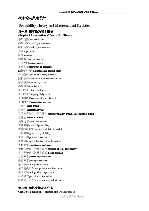
ProbabilityProf.F.P.KellyLent1996These notes are maintained by Andrew Rogers. Comments and corrections to soc-archim-notes@.Revision: 1.1Date:1998/06/2414:38:21The following people have maintained these notes.–June2000Kate MetcalfeJune2000–date Andrew RogersContentsIntroduction v 1Basic Concepts11.1Sample Space (1)1.2Classical Probability (1)1.3Combinatorial Analysis (2)1.4Stirling’s Formula (2)2The Axiomatic Approach52.1The Axioms (5)2.2Independence (7)2.3Distributions (8)2.4Conditional Probability (9)3Random Variables113.1Expectation (11)3.2Variance (14)3.3Indicator Function (16)3.4Inclusion-Exclusion Formula (18)3.5Independence (18)4Inequalities234.1Jensen’s Inequality (23)4.2Cauchy-Schwarz Inequality (26)4.3Markov’s Inequality (27)4.4Chebyshev’s Inequality (27)4.5Law of Large Numbers (28)5Generating Functions315.1Combinatorial Applications (34)5.2Conditional Expectation (34)5.3Properties of Conditional Expectation (36)5.4Branching Processes (37)5.5Random Walks (42)6Continuous Random Variables476.1Jointly Distributed Random Variables (50)6.2Transformation of Random Variables (57)6.3Moment Generating Functions (64)iiiiv CONTENTS6.4Central Limit Theorem (67)6.5Multivariate normal distribution (71)IntroductionThese notes are based on the course“Probability”given by Prof.F.P.Kelly in Cam-bridge in the Lent Term1996.This typed version of the notes is totally unconnected with Prof.Kelly.Other sets of notes are available for different courses.At the time of typing these courses were:Probability Discrete MathematicsAnalysis Further AnalysisMethods Quantum MechanicsFluid Dynamics1Quadratic MathematicsGeometry Dynamics of D.E.’sFoundations of QM ElectrodynamicsMethods of Math.Phys Fluid Dynamics2Waves(etc.)Statistical PhysicsGeneral Relativity Dynamical SystemsCombinatorics Bifurcations in Nonlinear Convection They may be downloaded from/maths/or/CambUniv/Societies/archim/notes.htm or you can email soc-archim-notes@ to get a copy of the sets you require.vCopyright(c)The Archimedeans,Cambridge University.All rights reserved.Redistribution and use of these notes in electronic or printed form,with or without modification,are permitted provided that the following conditions are met:1.Redistributions of the electronicfiles must retain the above copyright notice,thislist of conditions and the following disclaimer.2.Redistributions in printed form must reproduce the above copyright notice,thislist of conditions and the following disclaimer.3.All materials derived from these notes must display the following acknowledge-ment:This product includes notes developed by The Archimedeans,CambridgeUniversity and their contributors.4.Neither the name of The Archimedeans nor the names of their contributors maybe used to endorse or promote products derived from these notes.5.Neither these notes nor any derived products may be sold on a for-profit basis,although a fee may be required for the physical act of copying.6.You must cause any edited versions to carry prominent notices stating that youedited them and the date of any change.THESE NOTES ARE PROVIDED BY THE ARCHIMEDEANS AND CONTRIB-UTORS“AS IS”AND ANY EXPRESS OR IMPLIED WARRANTIES,INCLUDING, BUT NOT LIMITED TO,THE IMPLIED W ARRANTIES OF MERCHANTABIL-ITY AND FITNESS FOR A PARTICULAR PURPOSE ARE DISCLAIMED.IN NO EVENT SHALL THE ARCHIMEDEANS OR CONTRIBUTORS BE LIABLE FOR ANY DIRECT,INDIRECT,INCIDENTAL,SPECIAL,EXEMPLARY,OR CONSE-QUENTIAL DAMAGES HOWEVER CAUSED AND ON ANY THEORY OF LI-ABILITY,WHETHER IN CONTRACT,STRICT LIABILITY,OR TORT(INCLUD-ING NEGLIGENCE OR OTHERWISE)ARISING IN ANY WAY OUT OF THE USE OF THESE NOTES,EVEN IF ADVISED OF THE POSSIBILITY OF SUCH DAM-AGE.Chapter1Basic Concepts1.1Sample SpaceSuppose we have an experiment with a set of outcomes.Then is called the sample space.A potential outcome is called a sample point.For instance,if the experiment is tossing coins,then,or if the experi-ment was tossing two dice,then.A subset of is called an event.An event occurs is when the experiment is performed,the outcome satisfies.For the coin-tossing experiment,then the event of a head appearing is and for the two dice,the event“rolling a four”would be.1.2Classical ProbabilityIf isfinite,,and each of the sample points is“equally likely”then the probability of event occurring isExample.Choose digits from a table of random numbers.Find the probability that for,1.no digit exceeds,2.is the greatest digit drawn.Solution.The event that no digit exceeds isNow,so that.Let be the event that is the greatest digit drawn.Then.Also ,so that.Thus12CHAPTER1.BASIC CONCEPTSThe problem of the pointsPlayers A and B play a series of games.The winner of a game wins a point.The two players are equally skillful and the stake will be won by thefirst player to reach a target. They are forced to stop when A is within2points and B within3points.How should the stake be divided?Pascal suggested that the following continuations were equally likelyAAAA AAAB AABB ABBB BBBBAABA ABBA BABBABAA ABAB BBABBAAA BABA BBBABAABBBAAThis makes the ratio.It was previously thought that the ratio should beon considering termination,but these results are not equally likely.1.3Combinatorial AnalysisThe fundamental rule is:Suppose experiments are such that thefirst may result in any of possible out-comes and such that for each of the possible outcomes of thefirst experiments there are possible outcomes to experiment.Let be the outcome of experiment. Then there are a total of distinct-tuples describing the possible outcomes of the experiments.Proof.Induction.1.4Stirling’s FormulaFor functions and,we say that is asymptotically equivalent to and write if as.Theorem1.1(Stirling’s Formula).As,and thus.Wefirst prove the weak form of Stirling’s formula,that. Proof..Nowand,and soDivide by and let to sandwich between terms that tend to. Therefore.1.4.STIRLING’S FORMULA3Now we prove the strong form.Proof.For,we haveNow integrate from to to obtainLet.Then1we obtainFor,.Thus is a decreasing sequence,and.Therefore is bounded below,decreasing so is convergent.Let the limit be.We have obtainedWe need a trick tofind.Let.We obtain the recurrence by integrating by parts.Therefore and. Now is decreasing,soBut by substituting our formula in,we get thatTherefore as required.1by playing silly buggers with4CHAPTER1.BASIC CONCEPTSChapter2The Axiomatic Approach2.1The AxiomsLet be a sample space.Then probability is a real valued function defined on subsets of satisfying:-1.for,2.,3.for afinite or infinite sequence of disjoint events,.The number is called the probability of event.We can look at some distributions here.Consider an arbitraryfinite or countable and an arbitrary collection of non-negative numbers with sum.If we defineit is easy to see that this function satisfies the axioms.The numbers are called a probability distribution.If isfinite with elements,and ifwe recover the classical definition of probability.Another example would be to let and attach to outcome the probability for some.This is a distribution(as may be easily verified),and is called the Poisson distribution with parameter.Theorem2.1(Properties of).A probability satisfies1.,2.,3.if then,4..56CHAPTER2.THE AXIOMATIC APPROACH Proof.Note that,and.Thus.Now we can use this to obtain.If,write, so that.Finally,writeand.Then and,which gives the result.Theorem2.2(Boole’s Inequality).For any,Proof.Let and then inductively let.Thus the’s are disjoint and.ThereforeasTheorem2.3(Inclusion-Exclusion Formula).Proof.We know that.Thus the result is true for.We also have thatBut by distributivity,we haveApplication of the inductive hypothesis yields the result.Corollary(Bonferroni Inequalities).oraccording as is even or odd.Or in other words,if the inclusion-exclusion formula is truncated,the error has the sign of the omitted term and is smaller in absolute value. Note that the case is Boole’s inequality.2.2.INDEPENDENCE7 Proof.The result is true for.If true for,then it is true for and by the inductive step above,which expresses a-union in terms of two unions.It is true for by the inclusion-exclusion formula.Example(Derangements).After a dinner,the guests take coats at random from a pile.Find the probability that at least one guest has the right coat.Solution.Let be the event that guest has his1own coat.We want.Now,by counting the number of ways of matching guests and coats after have taken theirs.Thusand the required probability iswhich tends to as.Furthermore,let be the probability that exactly guests take the right coat. Then and is the number of derangements of objects.There-foreas2.2IndependenceDefinition2.1.Two events and are said to be independent ifMore generally,a collection of events,are independent iffor allfinite subsets.Example.Two fair dice are thrown.Let be the event that thefirst die shows an odd number.Let be the event that the second die shows an odd number andfinally let be the event that the sum of the two numbers is odd.Are and independent? Are and independent?Are,and independent?1I’m not being sexist,merely a lazy typist.Sex will be assigned at random...8CHAPTER2.THE AXIOMATIC APPROACH Solution.Wefirst calculate the probabilities of the events,,,,and.Event ProbabilityAs above,Thus by a series of multiplications,we can see that and are independent, and are independent(also and),but that,and are not independent.Now we wish to state what we mean by“2independent experiments”2.Consider and with associated probability distributionsand.Then,by“2independent experiments”,we mean the sample space with probability distribution.Now,suppose and.The event can be interpreted as an event in ,namely,and similarly for.Thenwhich is why they are called“independent”experiments.The obvious generalisation to experiments can be made,but for an infinite sequence of experiments we mean a sample space satisfying the appropriate formula.You might like tofind the probability that independent tosses of a biased coin with the probability of heads results in a total of heads.2.3DistributionsThe binomial distribution with parameters and,has and probabilities.Theorem2.4(Poisson approximation to binomial).If,withheldfixed,then2or more generally,.2.4.CONDITIONAL PROBABILITY9 Proof.Suppose an infinite sequence of independent trials is to be performed.Each trial results in a success with probability or a failure with probability.Such a sequence is called a sequence of Bernoulli trials.The probability that thefirst success occurs after exactly failures is.This is the geometric distribution with parameter.Since,the probability that all trials result in failure is zero.2.4Conditional ProbabilityDefinition2.2.Provided,we define the conditional probability of3to beWhenever we write,we assume that.Note that if and are independent then.Theorem2.5. 1.,2.,3.,4.the function restricted to subsets of is a probability function on. Proof.Results1to3are immediate from the definition of conditional probability.For result4,note that,so and thus. (obviously),so it just remains to show the last axiom.For disjoint’s,as required.3read“given”.10CHAPTER2.THE AXIOMATIC APPROACH Theorem2.6(Law of total probability).Let be a partition of.ThenProof.as required.Example(Gambler’s Ruin).A fair coin is tossed repeatedly.At each toss a gambler wins if a head shows and loses if tails.He continues playing until his capital reaches or he goes broke.Find,the probability that he goes broke if his initial capital is.Solution.Let be the event that he goes broke before reaching,and let or be the outcome of thefirst toss.We condition on thefirst toss to get.But and.Thus we obtain the recurrenceNote that is linear in,with,.Thus.Theorem2.7(Bayes’Formula).Let be a partition of.ThenProof.by the law of total probability.Chapter3Random VariablesLet befinite or countable,and let for.Definition3.1.A random variable is a function.Note that“random variable”is a somewhat inaccurate term,a random variable is neither random nor a variable.Example.If,then we can define random variables and by andLet be the image of under.When the range isfinite or countable then the random variable is said to be discrete.We write for,and forThenis the distribution of the random variable.Note that it is a probability distribution over.3.1ExpectationDefinition3.2.The expectation of a random variable is the numberprovided that this sum converges absolutely.1112CHAPTER3.RANDOM V ARIABLES Note thatAbsolute convergence allows the sum to be taken in any order.If is a positive random variable and if we write.Ifandthen is undefined.Example.If,then.Solution.Example.If then.3.1.EXPECTATION13 Solution.For any function the composition of and defines a new random variable and defines the new random variable given byExample.If,and are constants,then and are random variables defined byandNote that is a constant.Theorem3.1.1.If then.2.If and then.3.If and are constants then.4.For any random variables,then.5.is the constant which minimises.Proof. 1.meansSo2.If with and then,therefore.14CHAPTER3.RANDOM V ARIABLES 3.4.Trivial.5.NowThis is clearly minimised when.Theorem3.2.For any random variablesProof.Result follows by induction.3.2Variancefor Random Variable Standard DeviationTheorem3.3.Properties of Variance(i)if,thenProof-from property1of expectation(ii)If constants,3.2.V ARIANCE15 Proof.(iii)Proof.Example.Let X have the geometric distribution withand.Then and.Solution.Definition3.3.The co-variance of random variables and is:The correlation of and is:16CHAPTER3.RANDOM V ARIABLES Linear RegressionTheorem3.4.Proof.3.3Indicator FunctionDefinition3.4.The Indicator Function of an event is the functionif(3.1)ifNB that is a random variable1.2.3.4.if orWORKS!Example.couples are arranged randomly around a table such that males and fe-males alternate.Let=The number of husbands sitting next to their wives.Calculate3.3.INDICATOR FUNCTION17 the and the.event couple i are togetherThus18CHAPTER3.RANDOM V ARIABLES 3.4Inclusion-Exclusion FormulaTake Expectation3.5IndependenceDefinition3.5.Discrete random variables are independent if and only if for any:Theorem3.5(Preservation of Independence).If are independent random variables and are functionsthen are independent random variables3.5.INDEPENDENCE19 Proof.Theorem3.6.If are independent random variables then:NOTE that without requiring independence.Proof.Write for the range ofTheorem3.7.If are independent random variables and are func-tion then:Proof.Obvious from last two theorems!Theorem3.8.If are independent random variables then:20CHAPTER3.RANDOM V ARIABLES Proof.Theorem3.9.If are independent identically distributed random variables thenProof.Example.Experimental Design.Two rods of unknown lengths.A rule can measure the length but with but with error having0mean(unbiased)and variance. Errors independent from measurement to measurement.To estimate we could take separate measurements of each rod.3.5.INDEPENDENCE21 Can we do better?YEP!Measure as and asSo this is better.Example.Non standard dice.You choose1then I choose one.Around this cycle.So the relation’A better that B’is not transitive.22CHAPTER3.RANDOM V ARIABLESChapter4Inequalities4.1Jensen’s InequalityA function is convex if--Strictly convex if strict inequality holds whenf is concave if is convex.f is strictly concave if is strictly convex2324CHAPTER4.INEQUALITIES Concaveneither concave or convex.We know that if f is twice differentiable and for the if f is convex and strictly convex if for.Example.is strictly convex onExample.Strictly concave.Example.is strictly convex on but not onTheorem4.1.Let be a convex function.Then:,and.Further more if f is strictly convex then equality holds if and only if all x’s are equal.4.1.JENSEN’S INEQUALITY25 Proof.By induction on n nothing to prove definition of convexity. Assume results holds up to n-1.Consider,andFor set such thatThen by the inductive hypothesis twice,first for n-1,then for2f is strictly convex and not all the equal then we assume not all ofare equal.But thenSo the inequality is strict.Corollary(AM/GM Inequality).Positive real numbersEquality holds if and only ifProof.Letthen is a convex function on.So(Jensen’s Inequality)ThereforeFor strictness since f strictly convex equation holds in[1]and hence[2]if and only if26CHAPTER4.INEQUALITIES If is a convex function then it can be shown that at each pointa linear function such thatIf f is differentiable at y then the linear function is the tangentLet,andSo for any random variable X taking values in4.2Cauchy-Schwarz InequalityTheorem4.2.For any random variables,Proof.For LetThenquadratic in a with at most one real root and therefore has discriminant.4.3.MARKOV’S INEQUALITY27TakeCorollary.Proof.Apply Cauchy-Schwarz to the random variables and4.3Markov’s InequalityTheorem4.3.If X is any random variable withfinite mean then,for any aProof.LetTake expectation4.4Chebyshev’s InequalityTheorem4.4.Let X be a random variable with.ThenProof.28CHAPTER4.INEQUALITIES ThenTake ExpectationNote1.The result is“distribution free”-no assumption about the distribution of X(otherthan).2.It is the“best possible”inequality,in the following sensewith probabilitywith probabilitywith probabilityThen3.If then applying the inequality to givesOften the most useful form.4.5Law of Large NumbersTheorem4.5(Weak law of large numbers).Let be a sequences of inde-pendent identically distributed random variables with Variance LetThen,asW OF LARGE NUMBERS29 Proof.By Chebyshev’s Inequalityproperties of expectationSinceButThusExample.are independent events,each with probability p.Let. Thennumber of times A occursnumber of trialsTheorem states thatasWhich recovers the intuitive definition of probability.Example.A Random Sample of size n is a sequence of independent identically distributed random variables(’n observations’)is called the SAMPLE MEANTheorem states that provided the variance of isfinite,the probability that the sample mean differs from the mean of the distribution by more than approaches0as. We have shown the weak law of large numbers.Why weak?a strong form of larger numbers.asThis is NOT the same as the weak form.What does this mean?determinesas a sequence of real numbers.Hence it either tends to or it doesn’t.as30CHAPTER4.INEQUALITIESChapter5Generating FunctionsIn this chapter,assume that X is a random variable taking values in the range. LetDefinition5.1.The Probability Generating Function(p.g.f)of the random variable X,or of the distribution,isThis is a polynomial or a power series.If a power series then it is convergent for by comparison with a geometric series.Example.Theorem5.1.The distribution of X is uniquely determined by the p.g.f. Proof.We know that we can differential p(z)term by term forand soRepeated differentiation givesand has Thus we can recover from p(z)3132CHAPTER5.GENERATING FUNCTIONS Theorem5.2(Abel’s Lemma).Proof.For,is a non decreasing function of z and is bounded above by Choose,N large enough thatThenTrue and soUsually is continuous at z=1,then.RecallTheorem5.3.Proof.Proof now the same as Abel’s LemmaTheorem5.4.Suppose that are independent random variables with p.g.f’s.Then the p.g.f ofis33 Proof.Example.Suppose X has Poisson DistributionThenLet’s calculate the variance of XThenSince continuous atExample.Suppose that Y has a Poisson Distribution with parameter.If X and Y are independent then:But this is the p.g.f of a Poisson random variable with parameter.By uniqueness (first theorem of the p.g.f)this must be the distribution forExample.X has a binomial Distribution,34CHAPTER5.GENERATING FUNCTIONS This shows that.Where are independent random variables each withNote if the p.g.f factorizes look to see if the random variable can be written as a sum.5.1Combinatorial ApplicationsTile a bathroom with tiles.How many ways can this be done?SayLetSince,thenLetThe coefficient of,that is,is5.2Conditional ExpectationLet and be random variables with joint distribution5.2.CONDITIONAL EXPECTATION35 Then the distribution of X isThis is often called the Marginal distribution for.The conditional distribution for given by isDefinition5.2.The conditional expectation of X given is,The conditional Expectation of X given Y is the random variable defined byThusExample.Let be independent identically distributed random vari-ables with and.LetThenThenThereforeNote a random variable-a function of.36CHAPTER5.GENERATING FUNCTIONS 5.3Properties of Conditional ExpectationTheorem5.5.Proof.Theorem5.6.If and are independent thenProof.If and are independent then for anyExample.Let be i.i.d.r.v’s with p.g.f.Let N be a random variable independent of with p.g.f.What is the p.g.f of:Then for exampleExercise Calculate and henceIn terms of and5.4.BRANCHING PROCESSES37 5.4Branching Processessequence of random variables.number of individuals in the gener-ation of population.Assume.1.2.Each individual lives for unit time then on death produces offspring,probabil-ity.3.All offspring behave independently.Where are i.i.d.r.v’s.number of offspring of individual in generation. Assume1.2.Let F(z)be the probability generating function of.LetThen the probability generating function of the offspring distribution. Theorem5.7.is an n-fold iterative formula.38CHAPTER5.GENERATING FUNCTIONS Proof.Theorem5.8.Mean and Variance of population sizeIfandMean and Variance of offspring distribution.Then(5.1) Proof.Prove by calculating,Alternativelyby inductionThus5.4.BRANCHING PROCESSES39 Now calculateThenTo deal with extinction we need to be careful with limits as.LetExtinction occurs by generationand letthe event that extinction ever occursCan we calculate from?More generally let be an increasing sequenceand defineDefine for40CHAPTER5.GENERATING FUNCTIONS for are disjoint events andThusProbability is a continuous set function.Thusextinction ever occursSayNote,is an increasing sequence so limit exists.Butis the p.g.f ofSoAlsoSince F is continuousThus5.4.BRANCHING PROCESSES41“q”is called the Extinction Probability.Alternative DerivationTheorem5.9.The probability of extinction,,is the smallest positive root of the equa-tion.is the mean of the offspring distribution.If then while if thenProof.in Since AlsoThus if,there does not exists a with.If then letbe the smallest positive root of then.Further,Since is a root of42CHAPTER5.GENERATING FUNCTIONS 5.5Random WalksLet be i.i.d.r.vs.LetWhere,usuallyThen is a1dimensional Random Walk.We shall assumewith probability(5.2)with probabilityThis is a simple random walk.If then the random walk is called symmetricExample(Gambler’s Ruin).You have an initial fortune of and I have an initial fortune of.We toss coins repeatedly I win with probability and you win with probability.What is the probability that I bankrupt you before you bankrupt me?5.5.RANDOM WALKS43Set and Stop a random walk starting at when it hits or.Let be the probability that the random walk hits before it hits,starting from .Let be the probability that the random walk hits before it hits,starting from .After thefirst step the gambler’s fortune is either or with prob andrespectively.From the law of total probability.Also and.Must solve.orGeneral Solution for isand soIf,the general solution isTo calculate,observe that this is the same problem with replaced by respectively.Thusif44CHAPTER5.GENERATING FUNCTIONS orifThus and so on,as we expected,the game ends with probability one.hits beforeifOr ifWhat happens as?paths hit ever path hits before it hitshits ever hits beforeLet be the ultimate gain or loss.with probability(5.3)with probabilityif(5.4)ifFair game remains fair if the coin is fair then then games based on it have expected reward.Duration of a Game Let be the expected time until the random walk hits or,starting from.Isfinite?is bounded above by the mean of geometric random variables(number of window’s of size a before a window with all or ).Hence isfinite.Consider thefirst step.Thenduration durationfirst stepdurationfirst step up durationfirst step downEquation holds for with.Let’s try for a particular solutionfor。
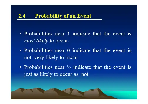
2. Probability (概率)2.1 Sample Space 样本空间statistical experiment (random experiment)----repeating----more than one outcome----know all the outcomes, but don ’t predict whichoutcome will be occurexample :toss an honest coin---- In this experiment there are only two possible outcomes:{head}, {tail}toss two honest coins---- In this experiment there are 4 possible outcomes:{H, H}, {H, T}, {T, H}, {T, T}Each outcome in a sample space is called a sample point of the sample space.Example 2.1.1 Consider the experiment of tossing a die. If we are interested in the number thatshows on the top face, the sample space would be{}11,2,3,4,5,6S =If we are interested only in whether the numbers is even or odd, the sample space is simply{}2,S even odd =Example 2.1.3 An experiment consists of flipping a coin and then flipping it a second time if ahead occurs. If a tail occurs on the first flip then a die is tossing once. To list the elements of thesample space providing the most information,we construct a diagram of Fig 2.1.1, which is called a tree diagram. Now the various paths alongthe branches of the tree give the distinct sample points. Starting with the top left branch andmoving to the right along the first path, we get the sample point HH, indicating the possibility thatheads occurs on two successive flips of the coin. The possibility that coin will show a tail followedby a 4 on the toss of the die is indicated by T4. Thus the sample space is{,,1,2,3,4,5,6}S HH HT T T T T T T =Fig .2.1.1 Tree diagram for Example 2.1.3 Definition 2.2.1 An event is a subset of a sample space.Example 2.2.1 Given the sample space {|0}S t t =≥. where t is the life in hours of a certainbulb, we are interest in the event B that a bulb burnt out before 200 hrs, i.e. the subset{|0200}B t t =≤< of S .Example 2.2.2 Assume that the unemployment rate r of a region is between 0 and 15%,i.e. wehave the sample space {|00.15}S r r =≤≤. If the event C “unemployment rate is low ”means that 0.04r ≤, then we have the subset {|00.04}C r r =≤≤ of S .You may have known operation of subsets, i.e.the complement of a subset (余集),the union of subset,(并集)the difference of subset (差集)intersection of subsets (交集),so we can say about the complement of an event, the union, difference and intersection ofevents.certain event (必然事件):The sample space S itself, is certainly an event, which is called a certain event, means thatit always occurs in the experiment.impossible event (不可能事件):The empty set, denoted by ∅, is also an event, called an impossible event, means that it neveroccurs in the experiment.Example 2.2.3 Consider the experiment of tossing a die, then{1,2,3,4,5,6}S =Let x be the number that shows on the top face, then the event {|,10}A x x S x =∈≤, isthe certain event, i.e. A S =.Then even {|,B x x S x =∈ is an irrational number }, (irrational-无理数)is the impossible event, i.e.B =∅.Let be the event consisting of all even numbers and be the event consisting of numbers divisible by 3. Find A , ,,A B A B A B .Solution We have {2,4,6,8},{3,6,9}.A B ==Thus{1,3,5,7,9}A = {2,3,4,6,8,9}A B = {6}A B = {3,9}A B = The relationship between events and the corresponding sample space can be illustrated graphical by means of Venn diagrams. In a Venn diagram, we represent the sample space by a rectangle and represent events by circles drawn inside the rectangle.Example 2.2.5 In Figure 2.2.1A B = regions 1 and 2, A D = regions 1,2 ,3 ,4 ,5 and 7,A B D = regions 2, 6 and 7A B D 1234567Fig 2.2.1 Venn diagram of Example 2.2.5The following list summarizes the rules of the operations of events.1. A ∅=∅2. A A ∅=3. A A A =4. A A =∅5. A A S =6. S =∅7. S ∅=8. A A =9. _________A B A B =10. _________A B A B =11. AB B A = 12. ()()AB C A B C = 13. ()()()AB C A C B C = 14. ()()()A B C A C B C =2.3 Probability of events1. relative frequency --------probability用频率定义概率Considering an Example.We plant 100 untreated cotton seeds.If 49 seeds germinate, that is, if there are 49 success (by success in statistics we mean the occurrence of the event under discussion) in 100 trials, we say that the relative frequency of success is 0.49.If we plant more and more seeds, a whole sequence of values for the respective relative frequencies is obtained. In general, these relative frequencies approach a limit value, we call this limit the probability of success in a single trial. From the data of Table 2.3.1 it appears that the relative frequencies are approaching the value 0.51, which we call the probability of a cotton seedling emerging from an untreated seed.relative frequencies are approaching the value 0.5252.0→n salways 1. Similarly, the probability of the impossible event is 0, and the probability of any event is always between 0 and 1.Note. In this definition , the word“limit”has a meaning which is different from the meaning you may have learned in calculus. We will discuss this problem later.Example 2.3.1Select 200 bulbs produced by company X at random of them 150 having life longer than 300hrs. Find the probability that the bulbs produced by company X have life longer than 300hrs.Solution.1500.75200p==Jixie-9-42.”equally likely to occur”------probability(古典概率,有限、等可能性)In many cases, the probability may be stated without experience. If we toss a properly balanced coin, we believe that the probability of getting a head is 0.5. We make this statement since in tossing a properly balanced coin, only two outcomes are possible and both outcome areIt should be pointed out that this definition is in a sense circular in nature, since the expression “equally likely to occur”itself involves the idea of probability. However, since this term is generally intuitively understood, the concept of “equally likely” will be left undefined.Solution.The sample space S consists of 20 sample points. The event {A= a white ball is drawn}consists of 4 sample points, thus the probability of drawing a white ball is4()0.2P A==.Solution The sample space is{S =(,)|,m n m n are positive integers 6}≤thus S consists of 36 sample points .Let {A =getting a total of 9},{B =getting a total greater of 9}Then we have{(3,6),(4,5),(5,4),(6,3)}A ={(4,6),(5,5),(6,4),(5,6),(6,5),(6,6)}B =Thus41()369P A == , 61()366P B ==. where ()p A is the probability that the event A occurs ./*******/Example 2.3.4 抽球问题Consecutively draw ballFrom a big pack which contains a white balls and b black balls, a ball is consecutively draw at random. what is the probability that the ball which be drawn in m-th time is white?抽球问题袋中有a 个白球,b 个黑球,从中依次任取一个球,且每次取出的球不再放回去,求第m 次取出的球是白球的概率。
Probability Theory and Mathematical Statistics1. OVERVIEW AND DESCRIPTIVE STATISTICS.Populations, Samples, and Processes.Pictorial and Tabular Methods in Descriptive Statistics.Measures of Location.Measures of Variability.2. PROBABILITY.Sample Spaces and Events.Axioms, Interpretations, and Properties of Probability.Counting Techniques.Conditional Probability.Independence.3. DISCRETE RANDOM VARIABLES AND PROBABILITY DISTRIBUTIONS. Random Variables.Probability Distributions for Discrete Random Variables.Expected Values of Discrete Random Variables.The Binomial Probability Distribution.Hypergeometric and Negative Binomial Distributions.The Poisson Probability Distribution.4. CONTINUOUS RANDOM VARIABLES AND PROBABILITY DISTRIBUTIONS.Continuous Random Variables and Probability Density Functions.Cumulative Distribution Functions and Expected Values.The Normal Distribution.The Exponential and Gamma Distribution.Other Continuous Distributions.Probability Plots.5. JOINT PROBABILITY DISTRIBUTIONS AND RANDOM SAMPLES.Jointly Distributed Random Variables.Expected Values, Covariance, and Correlation.Statistics and Their Distributions.The Distribution of the Sample Mean.The Distribution of a Linear Combination.6. POINT ESTIMATION.Some General Concepts of Point Estimation.Methods of Point Estimation.7. STATISTICAL INTERVALS BASED ON A SINGLE SAMPLE.Basic Properties of Confidence Intervals.Large-Sample Confidence Intervals for a Population Mean and Proportion.Intervals Based on a Normal Population Distribution.Confidence Intervals for the Variance and Standard Deviation of a Normal Population.8. TESTS OF HYPOTHESES BASED ON A SINGLE SAMPLE.Hypothesis and Test Procedures.Tests About a Population Mean.Tests Concerning a Population Proportion.P-Values.Some Comments on Selecting a Test.9. INFERENCES BASED ON TWO SAMPLES.z Tests and Confidence Intervals for a Difference Between Two Population Means. The Two-Sample t Test and Confidence Interval.Analysis of Paired Data.Inferences Concerning a Difference Between Population Proportions. Inferences Concerning Two Population Variances.10. THE ANALYSIS OF VARIANCE.Single-Factor ANOVA.Multiple Comparisons in ANOVA.More on Single-Factor ANOVA.11. MULTIFACTOR ANALYSIS OF VARIANCE.Two-Factor ANOVA with Kij = 1.Two-Factor ANOVA with Kij > 1.Three-Factor ANOVA.2p Factorial Experiments.12. SIMPLE LINEAR REGRESSION AND CORRELATION.The Simple Linear Regression Model.Estimating Model Parameters.Inferences About the Slope Parameter a1.Inferences Concerning Y-x* and the Prediction of Future Y Values. Correlation.13. NONLINEAR AND MULTIPLE REGRESSION.Aptness of the Model and Model Checking.Regression with Transformed Variables.Polynomial Regression.Multiple Regression Analysis.Other Issues in Multiple Regression.14. GOODNESS-OF-FIT TESTS AND CATEGORICAL DATA ANALYSIS. Goodness-of-Fit Tests When Category Probabilities are Completely Specified. Goodness of Fit for Composite Hypotheses.Two-Way Contingency Tables.15. DISTRIBUTION-FREE PROCEDURES.The Wilcoxon Signed-Rank Test.The Wilcoxon Rank-Sum Test.Distribution-Free Confidence Intervals.Distribution-Free ANOVA.16. QUALITY CONTROL METHODS.General Comments on Control Charts.Control Charts fort Process Location.Control Charts for Process Variation.Control Charts for Attributes.CUSUM Procedures.Acceptance Sampling.APPENDIX TABLES.Cumulative Binomial Probabilities.Cumulative Poisson Probabilities.Standard Normal Curve Areas.The Incomplete Gamma Function.Critical Values for t Distributions.Tolerance Critical Values for Normal Population Distributions.Critical Values for Chi-Squared Distributions. t Curve Tail Areas. Critical Values for F Distributions.Critical Values for Studentized Range Distributions.Chi-Squared Curve Tail Areas.Critical Values for the Ryan-Joiner Test of Normality.Critical Values for the Wilcoxon Signed-Rank Test.Critical Values for the Wilcoxon Rank-Sum Test.Critical Values for the Wilcoxon Signed-Rank Interval.Critical Values for the Wilcoxon Rank-Sum Interval. a Curves for t Tests. Answers to Odd-Numbered Exercises.Index.。
Chapter 2. Probability1.Sample spaceSample spaceIn the study of statistics we are concerned with the presentation and interpretation of chance outcomes that occur in a planned study or scientific investigation.For example, we may record the number of accidents that occur monthly at the intersection of Driftwood Lane and Royal Oak Drive, hoping to justify the installation of a traffic light; we might classify items coming of an assembly line as "defective" or "non defective"; or we may be interested in the volume of gas released in a chemical reaction when the concentration of an acid is varied.The statistician is often dealing with either experimental data, representing counts or measurements, or perhaps with categorical data that can be classified according to some criterion.We shall refer to any recoding of information, whether it be numerical or categorical, as an observation.The number 2, 0, 1 and 2, representing the number of accidents that occurred for each month from January through April during the past year at the intersection of Driftwood Lane and Royal Oak Drive, constitute a set of observations.The categorical data N, D, N, D and D,representing the items found to be defective or non defective when five items are inspected, are recorded as observations.experimentExperiment:any process that generates a set of data.tossing of a coin is a statistical experiment .There are only two possible outcomes, heads or tails.Another experiment might be the launching of a missile and observing its velocity at specified times.The opinions of voters concerning a new sales tax can also be considered as observations of an experiment.particularly interested in the observations obtained by repeating the experiment several times.example: a coin is tossed repeatedly• cannot predict the result of a given toss(i.e. the outcome depend on chance)• know the entire set of possibilities for each toss.Sample spaceDefinition 2.1 The set of all possible outcomes of a statistical experiment is called the sample space and is represented by S. Each outcome in a sample space is called an element or a sample point.What's the possible outcomes when a coin is tossed?The sample space may be writtenS ={H, T}H and T corresponds to 'heads' and 'tails', respectively.Example 2.1 Consider the experiment of tossing a die. interested in the number that shows on the top faceS1 ={}S={}S1provides more information than S2 If we know which elements in S1occurs, we can tell which outcome in S2 occurs; however, a knowledge of what happens in S2 is of little help in determining which element in S1 occurs.Remarks:• more than one sample space can be used to describe the outcomes of an experiment.• It is desirable to use a sample space that gives the most information.Example 2.3Suppose that three items are selected at random from a manufacturing process. Each item is inspected and classified defective, D, or non defective, N. List the elements of the sample space providing the most information.The sample space isS ={DDD, DDN, DND, DNN, NDD, NDN, NND, NNN}.sample space with a large or infinite number of sample points ,How to describe?by a statement or ruleexamples• S ={x | }• all points (x,y) on the boundary or the interior of a circle of radius 2 with center at the originsample space with a large or infinite number of sample points ,How to describe?by a statement or ruleexamples• S ={x | x is a city with a population over 1 million}• all points (x,y) on the boundary or the interior of a circle ofradius 2 with center at the origin{| x 2+ y 2≤}2.EventsEventFor any given experiment we may be interested in the occurrence of certain events rather than in the outcome of a specific element in the sample space.event A: the outcome (when a die is tossed) is divisible by 3.Event A will occur if the outcome is an element of the set A ={3, 6}A ={3, 6}is the subset of the sample spaceS1 ={}in Example 2.1.event B: the number of defectives is greater than 1 in Example 2.3; this will occur if the outcome is an element of the subsetB ={}Example 2.4.Given the sample space S ={t|t≥ 0}, where t is the life in years of a certain electronic component. Event A is that the component fails before the end of the fifth year.subset A ={t|0≤t < 5}Two special subseta subset that includes the entire sample space Sa subset contains no elements at all, denoted by ∅, called null set.{x|x is an even factor of 7}then B must be the null set, since the only possible factors of 7 are odd numbers 1 and 7.complementDefinition 2.3The complement of an event A with respect to S is the subset of all elements of S that are not in A. We denote the complement of A by the symbol A’Example 2.5 Let R be the event that a red card is selected from an ordinary deck of 52 playing cards and let S be the entire deck. What is R’?R’ is the event that the card selected from the deck is not red but a black card.intersectionoperations with events result in the formation of new eventsDefinition 2.4The intersection of two events A and B, denoted by the symbol A∩B, is the event containing all elements that are common to A and B.Example 2.7Let P be the event that a person selected at random while dining at a popular cafeteria is a taxpayer, and let Q be the event that the person is over 65 years of age. Then the event P∩Q is the set of all taxpayers in the cafeteria who are over 65 years of age.Example 2.8 Let M ={}and N ={r, s, t}; then it follows that M∩∅That is, M and N have no elements in common and, therefore, cannot both occur simultaneously.Definition 2.5 Two events A and B are mutually exclusive, or disjoint if A∩∅, that is, if A and B have no elements in common.UnionDefinition 2.6 The union of the two events A and B, denote by symbol A∪B, is the event containing all the elements that belong to A or B or both.Example 2.10 Let A ={a, b, c}{}; thenA∪{a, b, c, d, e}.Example 2.11 Let P be the event that an employee selected at random from an oil drilling company smokes cigarettes. Let Q be the event that the employee selected drinks alcoholic beverages. Then the event P∪Q is the set of all employees who either drink or smoke, or do both.Example 2.12If M ={x|3 < x < 9}{x|5 < x < 12}then M∪N ={x|3 < x < 12}Several resultsThe relationship between events and the corresponding sample space can be illustrated graphically by means of Venn diagrams.A∩∅∅,A∪∅= AA∩ A’= ∅,A∪A’= SS’=∅∅’=S(A’)’=A(A∩B)’=A’∪B’,(A∪B)’=A’∩B’3.Counting sample pointsOne the problems that the statistician must consider and attempt to evaluate is the element of chance associated with the occurrence of certain events when an experiment is performed.In many cases we shall be able to solve a probability problem by counting the number of points in the sample space without actually listing each element.Multiplication ruleTheorem 2.1 If an operation can be performed in n1 ways, and if for each of these a second operation can be performed in n2 ways, then the two operations can be performed together in n1n2ways.Example 2.13How many sample points are in the sample space when a pair of dice is thrown once?Solution The first dice can land in any one of n1= 6 ways. For each of these 6 ways the second die can also land in n2 = 6 ways. Therefore, the pair of dice can land in n1n2= 6× 6 = 36 possible ways.The multiplication rule of Theorem 2.1 may be extended to cover any number of operations.Theorem 2.2 If an operation can be performed in n1ways, and if for each of these a second operation can be performed in n2 ways, and for each of the first two a third operation can be performed i n 3 ways, and so forth, then the sequence of k operations can be performed in n1n2 . . n k ways.Example 2.15 Sam is going to assemble a computer by himself. He has the choice of ordering chips from two brands, a hard drive from four, memory from three and an accessory bundle from five local stores. How many different ways can Sam order the parts?Solution Since n1= 2,n2 = 4, n3 = 3, and n4 = 5, there aren1×n2×n3×n4 = 2×4×3×5 = 120different ways to order the parts.PermutationHow many different arrangements are possible for sitting 6 people around a table?How many different orders are possible for drawing 2 lottery tickets from a total of 20?The different arrangements are called permutation.Consider the three letters a, b, and c.The possible permutations are abc, acb, bac, bca, cab, and cba. There are 6 different arrangement.Using Theorem 2.2 we could arrive at the answer 6 without listing the diferent orders.There are n1 = 3 choices for the first position, then n2 = 2 forthe second, leaving only n3 = 1 choice for the last position, giving a total ofn1×n2×n3= 3×2×1 = 6 permutations.Theorem 2.3 The number of permutations of n distinct objects is n!.n ! is read 'n factorial'n! = n(n-1)(n-2)…(3)(2)(1)The number of permutations of the four letters a, b, c, and d will be 4! = 24.What's the number of permutations that are possible by taking the four letters two at a time?Using Theorem 2.1, we have n1 = 4 choices for the first position and n2 = 3 for the second.A total of n1n2 = 12 permutations.In general, n distinct objects taken r at a time can be arranged in n(n-1)(n-- r + 1) ways.Theorem 2.4 The number of permutations of n distinct objects taken r at a time isExample 2.17 Three awards (research, teaching and service) will be given one year for a class of 25 graduate students in a statistic department. If each student can receive at most one award, how many possible selections are there?Solution Since the awards are distinguishable, it is a permutation problem. The total number of sample points iscircular permutation:permutation that occur by arranging objects in a circleExample. 4 people are playing bridge, we do not have a new permutation if they all move one position in a clockwise direction.By considering one person in a fixed position and arranging the other three in 3! ways.Theorem 2.5 The number of permutations of n distinct objects arranged in a circle is (n-1)!combinationscombinations:the number of ways of selecting r objects from n without regard order. The number of such combinations is denoted by C r,nConsider the four letters a, b, c, and d.• the ways of selecting one letter from four? a , b, c, and d that is• the ways of selecting two letters from four? ab, ac, ad, bc, bd, cd; that is• the ways of selecting three letters from four?abc, abd, acd, bcd; that isTheorem 2.8 The number of combinations of n distinct objects taken r at a time isQuestion 1: What's the number of distinct permutations of n things of which n1 of one kind,n2 of a second kind,..., n k of a k th kind?hint: n objects, n positionsExample 2.19In a college football training session, the defensive coordinator needs to have 10 player standing in a row. Among these 10 players, there are 1 freshman, 2 sophomore, 4 juniors and 3 seniors, respectively. How many different ways can they be arranged in a row if only their class level will be distinguished?Solution The total number of arrangements isQuestion 2: What's the number of arrangements of a set of n objects into r cells with n1 elements in the first cell, n2elements in the second, and so forth?Example 2.20In how many ways can 7 scientists be assigned to one triple and two double hotel rooms?Solution: The total number of possible partitions would be4. Probability of an EventPerhaps it was man's unquenchable thirst for gambling that led to the early development of probability theory. In an effort to increase their winnings, gamblers called upon mathematicians to provide optimum strategies for various games of chance. Some of the mathematicians providing these strategies were Pascal, Leibniz, Fermat, and James Bernoulli.Probability theory has branched out far beyond games of chance to encompass many other fields associated with chance occurrences, such as politics, business, weather forecasting, and scientific research.probabilityThe remainder of chapter 2 only consider sample space contains a finite number of elementsTo every point in the sample space we assign a probability such that the sum of all probabilities is 1.The probability of an event A is denoted by P (A).Definition 2.8 The probability of an event A is the sum of the weights of all sample points in A. Therefore,0≤P (A)≤1, P (∅) = 0 P (S) = 1,Furthermore, if A1, A2, A3,…is a sequence of mutually exclusive events, thenExample 2.22 A coin is tossed twice. What is the probability that at least one head occurs?Solution The sample space is S ={HH, HT, T H, T T}The coin is balanced, each of these outcomes would be equally likely to occur. That is, the probability of each sample point is 1/4.event A: at least one head occurring. A ={HH, HT, T H}Example 2.23 A dice is loaded in such a way that an even number is twice as likely to occur as an odd number. If E is the event that a number less than 4 occurs on a single toss of the die, find P (E).Solution The sample space is S ={1, 2, 3, 4, 5, 6}assign a probability of w to each odd number, and 2 to each even number, we have 9 w= 1.1/ 9 , and 2/9 are assigned to each odd and even number, respectively.Since E ={1, 2, 3}Example 2.24In Example 2.23 let A be the event that an even number turns up and let B be the event that a number divisible by 3 occurs. Find P (A∪B) and P (A∩B)Solution We can get A ={2, 4, 6}{3, 6}, therefore,A∪B ={2, 3,4, 6}and A∩ B ={6}assign: 1/ 9→each odd number, 2/9→ each even number,we haveIf the sample space contains N elements, all of which are equally likely to occur, We assign 1/N to each element.Event A containing n of these N sample points. P (A)?Theorem 2.9 If an experiment can result in any one of N different equally likely outcomes, and if exactly n of these outcomes correspond to event A, then the probability of event A isExample 2.25 A statistic class for engineers consists of 25 industrial, 10 mechanical, 10 electrical, and 8 civil engineering students. If a person is randomly selected by the instructor to answer a question, find the probability that the student chosen is (a) an industrial engineering major, (b) a civil engineering or an electrical engineering major.SolutionDenote by I, M, E, and C the students majoring in industrial, mechanical, electrical and civil engineering, respectively. students in the class: equally to be selected;the total number: 53.(a) Since 25 of the 53 students are majoring in industrial engineering, the probability of the event I is(b) Since 18 of the 53 students are civil and electrical engineering majors, it follows thatExample 2.26In a poker hand consisting of 5 cards, find the probability of holding 2 aces and 3 jacks.SolutionThe number of ways of being dealt 2 aces from 4 isThe number of ways of being dealt 3 jacks from 4 isBy the multiplication rule of Theorem 2.1, there are n = 6× 4 = 24 hands with 2 aces and 3 jacks.The total number of 5-card poker hands isTherefore, the probability of event C of getting 2 aces and 3 jacks in a 5-card poker hand isIf event A occurs n A times in N repeated experiments under a certain conditions, then frequency of A occurring in N experiments is defined as:When N is large enough, the frequency turns out to have a kind of stability.i.e., the values of F N (A) show fluctuations which become progressively weaker as N increases, until ultimately F N (A) stabilizes to a constant.Tossing a fair coin, let A ={head comes up}Frequency stabilizes to 1/2The statistical definition of probability:The constant to which the frequency of the event A stabilizes is called the probability of the occurrence of event A (P (A).5. Additive RulesOften it is easier to calculate the probability of some event from other events.the event in question can be represented as the union of two other events, or as the complement of some event.Lay out several important laws that simplify the computation of probabilities.Additive Rulesadditive ruleTheorem 2.10If A and B are any two events, thenP (A∪B) = P (A) + P (B)-P (A∩B).PROOF. Use the V enn diagram.Corollary 2 If A1, A2, . . , A n are mutually exclusive, thenP (A1∪A2∪. . , ∪A n) = P (A1) + P (A2) + . . + P (A n ).a partition of S1.{A1, A2, . . , A n }2. A1, A2, . . , A n are mutually exclusive and A1∪A2∪. . , ∪A n= S.Corollary 3If{A1, A2, . . , A n }is a partition of S, thenP (A1∪A2∪. . , ∪A n) =P (A1) + P (A2) + . . + P (A n ) = P (S) = 1Example 2.27John is going to graduate from an industrial engineering department in a university by the end of the semester. After being interviewed at two companies he likes, he assesses that his probability of getting an offer from company A is 0.8, and the probability he gets an offer from company B is 0.6. If, on the other hand, he believes that the probability that he will get offers from both companies is 0.5.What is the probability that he will get at least one offer from these two companies?Solution Using the additive rule we haveP (A∪B) = P (A) + P (B)-P (A∩B) = 0.8 + 0.6-0.5 = 0.9.Example 2.28What is the probability of getting a total of 7 or 11 when a pair of fair dice are tossed?SolutionA: the event that 7 occurs; B: the event that 11 occurs.● a total of 7 occurs for 6 of the 36 sample points and a total of 11 occurs for only 2 of the sample points.●all sample points are equally likely, we have P (A) = 1/6 and P (B) = 1/18.The events A and B are mutually exclusive, therefore(此时两件事件不能同时发生!)How about the union of 3 events?Theorem 2.11 For three events A, B, and C,P (A∪B∪C) = P (A) + P (B) + P (C)-P (A∩B) -P (A∩ C)-P (B∩C) + P (A∩ B∩C). How to prove?Sometimes, it is more difcult to calculate the probability that an event occurs than it is to calculate the probability that the event does not occur.Theorem 2.12 If A and A ’ are complementary events, then P (A) + P (A’) = 1.Example 2.30If the probabilities that an automobile mechanic will service 3,4,5,6,7, or 8 or more cars on any given workday are, respectively, 0.12, 0.19, 0.28, 0.24, 0.10 and 0.07, what is the probability that he will service at least 5 cars on his next day at work?Solution. Let E be the event that at least 5 cars are serviced.Now, P (E) = 1 - P (E’), where E’ is the event that fewer than 5 cars are serviced.P (E’) = 0.12 + 0.19 = 0.31, it follows that P (E) = 1-0.31 = 0.69.6. Conditional ProbabilityConditional ProbabilityThe probability of an event B occurring when it is known that some event A has occurred.denoted by P (B|A), read "the probability of B, given A".ExampleA die is constructed such that the even numbers are twice as likely to occur as the odd numbers.i.e. the sample space is S ={1, 2, 3, 4, 5, 6}event B: get a perfect square when a die is tossed. the probability that B occurs: P (B) = 1/3.If it is known that the toss of the die resulted in a number greater than 3. What's the probability that B occurs under this condition?{4, 5, 6}, a subset of S.to find the probability that B occurs, relative to the space A, denote this event by B|A,B|A ={4}Remark: Events may have different probabilities when considered relative to different sample spaces.We can also writeP (A∩B) and P (A): from the original sample space S.Definition 2.9The conditional probability of B, given A, denoted by P (B|A), is defined bya conditional probability relative to a subspace A of S may be calculated directly from the probabilities assigned to the elements of the original sample space S.Example 2.31The probability that a regularly scheduled flight departs on time is P (D) = 0.83; the probability that it arrives on time is P (A) = 0.82; and the probability that it departs and arrives on time is P (D∩A) = 0.78. Find the probability that a plane(a) arrives on time given that it departed on time,(b) departed on time given that it has arrived on time.Solutiona.b.It is important to know the probability that the flight arrives on time. One is given the information that the flight did not depart on time. Armed with this additional information, the more pertinent probability is P(A|D’).(注:A∩D’∪A∩D=A)The probability of an on-time arrival is diminished severely in the presence of the additional information. The probability P (A|D’) is an "updating" of P (A) based on the knowledge that event D’has occurred.Independent Eventsprevious example: the die-tossing experiment.we have P(B|A) = 2/5, P (B) = 1/3.,P (B|A)= P (B), indicating that B depends on A.Example 2 cards are drawn in succession from an ordinary deck, with replacement.A: the first card is an ace,B: the second card is a spade.Since the first card is replaced, our sample space for both the first and second draws is the same.P (B|A) = 13/52 and P (B) = 13/52.We have P (B|A) = P (B), the events A and B are said to be independent.Definition 2.10Two events A and B are independent if and only ifP (B|A) = P (B) or P (A|B) = P (A). Otherwise, A and B are dependent.Remark The condition P(B|A) = P (B) implies that P (A|B) = P (A), and conversely.7. Multiplicative RulesMultiplicative RulesMultiplying the formula of Definition 2.9 by P (A), we obtain the multiplicative ruleTheorem 2.13 If in an experiment the events A and B can both occur, thenP (A∩B) = P (A)P (B|A).We can also write P (A∩B)= P (B)P (A|B).Example 2.32Suppose that we have a fuse box containing 20 fuses, of which 5 are defective. If 2 fuses are selected at random and removed from the box in succession without replacing the first, what is the probability that both fuses are defective?Solutionevent A: the first fuse is defectiveevent B: the second fuse is defectiveA∩B: A occurs, and then B occurs after A has occurredExample 2.33 One bag contains 4 white balls and 3 black balls, and a second bag contains 3 white balls and 5 black balls. One ball is drawn from the first bag and placed unseen in the second bag. What is the probability that a ball now drawn from the second bag is black?Solution B1: a black ball from bag 1;B2: a black ball from 2;W1: a white ball from bag 1.If the first fuse is replaced in Example 2.32, then the probability of a defective fuse on the second selection is still 1/4.i.e. P (B|A) = P (B) = 1/4. The events A and B are independent.Theorem 2.14 Two events A and B are independent if and only if P (A∩B) = P (A)P (B).Example 2.34 A small town has one fire engine and one ambulance available for emergencies. The probability that the fire engine is available when needed is 0.98, and the probability that the ambulance ia available when called is 0.92. In the event of an injury resulting from a burning building, find the probability that both the ambulance and the fire engine will be available. Solution Let A and B represent the respective events that the fire engine and the ambulance are available. ThenP (A∩B) = P (A)P (B) = 0.98×0.92 = 0.9016Theorem 2.15 If the events A1, A2, A3, …Ak can occur,then P (A1∩A2∩A3∩ …∩Ak) = P (A1)P (A2|A1)P (A3|A1∩A2)… P (A k|A1∩A2∩A3∩ …∩Ak-1)Example 2.36 Three cards are draw in succession, without replacement, from an ordinary deck of playing cards. Find the probability that the event A1∩A2∩A3occurs, where A1 is the event that the first card is a red ace, A2 the second card is a 10 or a jack, and A3is the event that is the event that the third card is greater than 3 but less than 7.Solution We have P (A1) = 2/52, P (A2|A1) = 8/51, P (A3|A1∩A2) = 12/50,by Theorem 2.15 : P (A1∩A2∩A3 )= P (A1) P (A2|A1)P(A3|A1∩A2) = 8/5525.Example 2.37A coin is biased so that a head is twice likely to occur as a tail. If the coin is tossed 3 times, what is the probability of getting 2 tails and 1 head?Solution the sample space{}P (H) = 2/3, P (T ) = 1/3event A: get 2 tails and 1 head; A ={T T H, T HT, HT T}P (T T H) = P (T )P (T )P (H) = ( 1/3)(1/3 )(2/3 ) = 2/27.Similarly, P (T HT ) = P (HT T ) = 2/27,P (A) = 2/27 + 2/27 + 2/27 = 2/9.8. Bayes' RuleP (A) = P [(E∩A)∪(E∩A)] = P (E∩A) + P (E∩A)= P (E)P (A|E) + P (E’)P (A|E’) draw the Venn diagramBayes' RuleA generalization,theorem of total probabilityTheorem 2.16 If the events B1, B2, . . . , Bkconstitute a partition of the sample space S such that P (Bi)≠0 fori = 1 ,2 ..,,.,k, then for any event A of SExample 2.38In a certain assembly plant, three machines, B1, B2,B3make 30%, 45%, and 25%, respectively, of the products. It is known from past experience that 2%, 3% and 2% of the products made by each machine, respectively, are defective. Suppose that a finished products is randomly selected. What is the probability that it is defective?Solution Applying Theorem 2.16, i.e. the theorem of total probability, we can writeP (A) = P (B1)P (A|B1) + P (B2)P (A|B2) + P (B3)P (A|B3).On the other hand,P (B1)P (A|B1) = 0.3×0.02 = 0.006,P (B2)P (A|B2) = 0.45×0.03 = 0.0135,P P (B3)P (A|B3).= 0.25×0.02 = 0.005.Therefore,P (A) = 0.006 + 0.0135 + 0.005 = 0.0245Example 2.39With reference to Example 2.38, if a product were chosen randomly and found to be defective, what is the probability that it was made by machine B3?SolutionTheorem 2.17 (Bayes' Rule)If the events B1, B2, . . . , Bkconstitute a partition of the sample space S, where P (Bi)≠0 for i = 1, 2, . . . , k, then for any eventA in S such that P (A)≠0,Exercises for Chapter 21. A truth serum has the property that 90% of the guilty suspects are properly judged while, of course, 10% of guilty suspects are improperly found innocent. On the other hand, innocent suspects are misjudged 1% of the time. If the suspect was selected from a group of suspects of which only 5% have ever committed a crime, and the scrum indicates that he is guilty, what is the probability that he is innocent?3. By comparing appropriate regions of Venn diagrams(a) (A∩B)∪(A∩B’) =?5. How many bridge hands are possible containing 4 spades, 6 diamonds, 1 club, and 2 hearts?7. A large industrial firm uses 3 local motels to provide overnight accommodations for its clients. From past experience it is known that 20% of the clients are assigned rooms at the Ramada Inn, 50% at the Sheraton, and 30% at the Lakeview Motor Lodge. If the plumbing is faulty in 5% of the rooms at the Ramada Inn, in 4% of the rooms at the Sheraton, and in 8% of the rooms at the Lakeview Motor Lodge, what is the probability that(a) a client will be assigned a room with faulty plumbing?(b) a person with a room having faulty plumbing was assigned accommodations at the Lakeview Motor Lodge?9. The probability that a patient recovers from a delicate heart operation is 0.8. What is the probability that(a) exactly 2 of the next 3 patients who have this operation survive?(b) all of the next 3 patients who have this operation survive?11. From 4 red, 5 green, and 6 yellow apples, how many selections of 9 apples are possible if 3 of each color are to be selected?13. A shipment of 12 television sets contains 3 defective sets. In how many ways can a hotel purchase 5 of these sets and receive at least 2 of the defective sets?15. A certain federal agency employs three consulting firms (A, B, and C) with probabilities 0.40, 0.35, and 0.25, respectively. From past experience it is known that the probability of cost overruns for the firms are 0.05, 0.03, and 0 .15, respectively. Suppose a cost overrun is experienced by the agency.(a) What is the probability that the consulting firm involved is company C?(b) What is the probability that it is company A?。