MULTIPRED a computational system for prediction of

Querying Very Large Multi-dimensional Datasets in ADR-Extended AbstractTahsin Kurc,Chialin Chang,Renato Ferreira,Alan Sussman,Joel Saltz Institute for AdvancedComputer StudiesandDept.of Computer Science University of Maryland College Park,MD20742Dept.of Pathology Johns Hopkins MedicalInstitutions Baltimore,MD21287kurc,chialin,renato,als,saltz@1IntroductionAnalysis and processing of very large multi-dimensional scientific datasets(i.e.where data items are associated with points in a multi-dimensional attribute space)is an important component of science andengineering.Moreover,an increasing number of applications make use of very large multi-dimensional datasets.Examples of such datasets include raw and processed sensor data from satellites[12],output fromhydrodynamics and chemical transport simulations[10],and archives of medical images[1].Many applications that make use of multi-dimensional datasets have several important characteristics. Both the input and the output are often disk-resident datasets.Applications may use only a subset of all thedata available in input and output datasets.Access to data items is described by a range query,namely a multi-dimensionalbounding box in the underlying multi-dimensionalattribute space of the dataset.Only thedata items whose associated coordinates fall within the multi-dimensional box are retrieved.The processing structures of these applications also share common characteristics.Figure1shows high-level pseudo-codefor the basic processing loop in these applications.The processing steps consist of retrieving input and output data items that intersect the range query(steps1–2and4–5),mapping the coordinates of the retrievedinput items to the corresponding output items(step6),and aggregating,in some way,all the retrieved input items mapped to the same output data items(steps7–8).Correctness of the output usually does not dependon the order input data items are aggregated.The mapping function,,maps an input item to a set of output items.An intermediate data structure,referred to as an accumulator,is used to hold intermediate results during processing.For example,an accumulator can be used to keep a running sum for an averagingoperation.The aggregation function,,aggregates the value of an input item with the intermediate result stored in the accumulator element().The output dataset from a query is usually much smaller than the input dataset,hence steps4–8are called the reduction phase of the processing.Accumulator elements are allocated and initialized(step3)before the reduction phase.Another constraint is that there isOutput Dataset,Input Dataset(*Initialization*)1.foreach in do2.read3.(*Reduction*)4.foreach in do5.read6.7.foreach in do8.(*Output*)9.foreach do10.11.writeFigure1:The basic processing loop in the target applications.a one-to-one mapping between output items and accumulator elements.The intermediate results stored in the accumulator are post-processed to producefinal results(steps9–11).Typical examples of application classes that make use of multi-dimensional scientific datasets are satellite data processing applications[15,5],the Virtual Microscope and analysis of microscopy data[1], and simulation systems for water contamination studies[10].Due to limited space,we briefly describe the satellite data processing application here.In satellite data processing,earth scientists study the earth by processing remotely-sensed data continuously acquired from satellite-based sensors.Each sensor reading is associated with a position(longitude and latitude)and the time the reading was recorded.In a typical analysis[15],a range query defines a bounding box that covers a part or all of the surface of the earth over a period of time.Data items retrieved from one or more datasets are processed to generate one or more composite images of the area under study.Generating a composite image requires projection of the selected area of the earth onto a two-dimensional grid[18];each pixel in the composite image is computed by selecting the“best”sensor value that maps to the associated grid posite images can be added to the database as new datasets.We have developed an infrastructure,called the Active Data Repository(ADR)[3],that integrates stor-age,retrieval and processing of large multi-dimensional datasets on distributed memory parallel architectures with multiple disks attached to each node.ADR targets applications with the processing structure shown in Figure1.ADR is designed as a set of modular services implemented in C++.Through use of these services, ADR allows customization for application specific processing(i.e.the,,,and functions),while providing support for common operations such as memory management,data retrieval,and scheduling of processing across a parallel machine.The system architecture of ADR consists of a front-end and a parallel back-end.The front-end interacts with clients,and forwards range queries with references to user-defined processing functions to the parallel back-end.During query execution,back-end nodes retrieve input data and perform user-defined operations over the data items retrieved to generate the output products.Output products can be returned from the back-end nodes to the requesting client,or stored in ADR.Several runtime support libraries andfile systems have been developed to support efficient I/O in a parallel environment[2,6,8,9,13,14,16,17].ADR differs from these systems in several ways.First, ADR is able to carry out range queries directed at irregular spatially indexed datasets.Second,computation is an integral part of the ADR framework.With the collective I/O interfaces provided by many parallel I/O systems,data processing usually cannot begin until the entire collective I/O operation completes.Third, data placement algorithms optimized for range queries are integrated as part of the ADR framework.In this work,we discuss optimizing the execution of range queries(i.e.the processing loop shown in Figure1)on distributed memory parallel machines within the ADR framework.We describe three potential strategies for efficient execution of such queries.We evaluate scalability of these strategies for different application scenarios,varying both the number of processors and the input dataset size,using application emulators[19]to generate various application scenarios for the applications classes that motivated the design of ADR.We present experimental evaluation of the three strategies on a128-node IBM SP.2Query Execution in ADR2.1Storing Datasets in ADRA dataset is partitioned into a set of chunks to achieve high bandwidth data retrieval.A chunk consists of one or more data items,and is the unit of I/O and communication in ADR.That is,a chunk is always retrieved as a whole during query processing.As every data item is associated with a point in a multi-dimensional attribute space,every chunk is associated with a minimum bounding rectangle(MBR)that encompasses the coordinates(in the associated attribute space)of all the items in the chunk.Since data is accessed through range queries,it is desirable to have data items that are close to each other in the multi-dimensional space in the same chunk.Chunks are distributed across the disks attached to ADR back-end nodes using a declustering algorithm[7,11]to achieve I/O parallelism during query processing.Each chunk is assigned to a single disk,and is read and/or written during query processing only by the local processor to which the disk is attached.If a chunk is required for processing by one or more remote processors,it is sent to those processors by the local processor via interprocessor communication.After all data chunks are stored into the desired locations in the disk farm,an index(e.g.,an R-tree)is constructed using the MBRs of the chunks.The index is used by the back-end nodes tofind the local chunks with MBRs that intersect the range query.2.2Query PlanningA plan specifies how parts of thefinal output are computed and the order the input data chunks are retrieved for processing.Planning is carried out in two steps;tiling and workload partitioning.In the tiling step, if the output dataset is too large tofit entirely into the memory,it is partitioned into tiles.Each tile,, contains a distinct subset of the output chunks,so that the total size of the chunks in a tile is less than the amount of memory available for output data.Tiling of the output implicitly results in a tiling of the input dataset.Each input tile,,contains the input chunks that map to the output chunks in tile,.During query processing,each output tile is cached in main memory,and input chunks from the required input tiles are retrieved.Since a mapping function may map an input element to multiple output elements,an input chunk may appear in more than one input tile if the corresponding output chunks are assigned to different tiles. Hence,an input chunk may be retrieved multiple times during execution of the processing loop.Figure2 illustrates the processing loop with tiled input and output datasets.In the workload partitioning step,the workload associated with each tile(i.e.aggregation of items in input and accumulator chunks)is partitioned across processors.This is accomplished by assigning each(*Output and Input Dataset Tiles*)and for11.foreach in,do(*Initialization*)2.foreach in do3.read4.(*Reduction*)5.foreach in do6.read7.8.foreach in do9.(*Output*)10.foreach do11.12.writeFigure2:Basic processing loop with tiled input and output datasets.is the total number of tiles after tiling step.processor the responsibility for processing a subset of the input and/or accumulator chunks.2.3Query ExecutionThe processing of a query on a back-end processor progresses through four phases for each tile:1.Initialization.Accumulator chunks in the current tile are allocated space in memory and initialized.If an existing output dataset is required to initialize accumulator elements,an output chunk is retrieved by the processor that has the chunk on its local disk,and the chunk is forwarded to the processors that require it.2.Local Reduction.Input data chunks on the local disks of each back-end node are retrieved andaggregated into the accumulator chunks allocated in each processor’s memory in phase1.3.Global Combine.If necessary,results computed in each processor in phase2are combined acrossall processors to computefinal results for the accumulator chunks.4.Output Handling.Thefinal output chunks for the current tile are computed from the correspondingaccumulator chunks computed in phase3.If the query creates a new dataset,output chunks are declustered across the available disks,and each output chunk is written to the assigned disk.If the query updates an already existing dataset,the updated output chunks are written back to their original locations on the disks.A query iterates through these phases repeatedly until all tiles have been processed and the entire output dataset has been computed.Note that the reduction phase in Figure2is divided into two phases,localreduction and global combine.This is a result of workload partitioning for parallel query execution,as will be discussed in Section3.To reduce query execution time,ADR overlaps disk operations,network operations and processing as much as possible during query processing.Overlap is achieved by maintaining explicit queues for each kind of operation(data retrieval,message sends and receives,data processing)and switching between queued operations as required.Pending asynchronous I/O and communication operations in the operation queues are polled and,upon their completion,new asynchronous operations are initiated when more work is expected and memory buffer space is available.Data chunks are therefore retrieved and processed in a pipelined fashion.3Query Processing StrategiesIn this section we briefly describe three strategies that use different tiling and workload partitioning ap-proaches.More detailed descriptions of these strategies can be found in[4].We refer to an input/output data chunk stored on one of the disks attached to a processor as a local chunk on that processor.Otherwise, it is a remote chunk.A processor owns an input or output chunk if it is a local input or output chunk.A ghost chunk is a copy of an accumulator chunk allocated in the memory of a processor that does not own the corresponding output chunk.In the tiling phase of all the strategies described in this section,we use a Hilbert space-filling curve[7] to create the tiles.The goal is to minimize the total length of the boundaries of the tiles,by assigning chunks that are spatially close in the multi-dimensionalattribute space to the same tile,to reduce the number of input chunks crossing tile boundaries.The advantage of using Hilbert curves is that they have good clustering properties[11],since they preserve locality.In our implementation,the mid-point of the bounding box of each output chunk is used to generate a Hilbert curve index.The chunks are sorted with respect to this index,and selected in this order for tiling.The current implementation,however,does not explicitly take into account the mapping between the input and output chunks,and therefore in some cases there can still be many input chunks intersecting multiple tiles,despite a small boundary length.3.1Fully Replicated Accumulator(FRA)StrategyIn this scheme each processor performs processing associated with its local input chunks.The output chunks are partitioned into tiles,each of whichfits into the available local memory of a single back-end processor. When an output chunk is assigned to a tile,the corresponding accumulator chunk is put into the set of local accumulator chunks in the processor that owns the output chunk,and is assigned as a ghost chunk on all other processors.This scheme effectively replicates all of the accumulator chunks in a tile on each processor,and during the local reduction phase,each processor generates partial results for the accumulator chunks using only its local input chunks.Ghost chunks with partial results are then forwarded to the processors that own the corresponding output(accumulator)chunks during the global combine phase to produce the complete intermediate result,and eventually thefinal output product.3.2Sparsely Replicated Accumulator(SRA)StrategyThe FRA strategy replicates each accumulator chunk in every processor even if no input chunks will be aggregated into the accumulator chunks in some processors.This results in unnecessary initialization overhead in the initialization phase of query execution,and extra communication and computation in the global combine phase.The available memory in the system also is not efficiently employed,because ofunnecessary replication.Such replication may result in more tiles being created than necessary,which may cause a large number of input chunks to be retrieved from disk more than once.In SRA strategy,a ghost chunk is allocated only on processors owning at least one input chunk that projects to the corresponding accumulator chunk.The index,which contains the MBRs of all the chunks,is used to decide where ghost chunks need to be allocated.Note that the index is constructed when the dataset is loaded into ADR.3.3Distributed Accumulator(DA)StrategyIn this scheme,every processor is responsible for all processing associated with its local output chunks. Tiling is done by selecting from each processor its local output chunks until the memory space allocated for the corresponding accumulator chunks isfilled.As in the other schemes,output chunks are selected in Hilbert curve order.Since no accumulator chunks are replicated by the DA strategy,no ghost chunks are allocated.This allows DA to make more effective use of memory and produce fewer tiles than the other two schemes.As a result,fewer input chunks are likely to be retrieved for multiple tiles.Furthermore,DA avoids interprocessor communication for accumulator chunks during the initialization phase and for ghost chunks during the global combine phase,and also requires no computation in the global combine phase.The FRA and SRA strategies eliminate interprocessor communication for input chunks,by replicating all accumulator chunks.On the other hand,the distributed accumulator strategy introduces communication in the local reduction phase for input chunks;all the remote input chunks that map to the same output chunk must be forwarded to the processor that owns the output chunk.Since a projection function may map an input chunk to multiple output chunks,an input chunk may be forwarded to multiple processors.In addition,a good declustering strategy could cause almost all input chunks to be forwarded to other processors,because an input chunk and the output chunk(s)that it projects to are unlikely to be assigned to the same processor.4Experimental ResultsWe present an experimental evaluation of the three query execution strategies on a128-node IBM SP multicomputer.Each node of the SP is a thin node with256MB of memory;the nodes are connected via a High Performance Switch that provides110MB/sec peak communication bandwidth per node.Each node has one local disk with500MB of available scratch space.We allocated225MB of that space for the input dataset and25MB for the output dataset for these experiments.The AIXfilesystem on the SP nodes uses a main memoryfile cache,so we used the remaining250MB on the disk to clean thefile cache before each experiment to obtain more reliable performance results.We evaluate the query execution strategies for different application scenarios,varying the number of processors and the input dataset size.We used application emulators[19]to generate various application scenarios for the applications classes that motivated the design of ADR(see Section1).An application emulator provides a parameterized model of an application class;adjusting the parameter values makes it possible to generate different application scenarios within the application class and scale applications in a controlled way.The assignment of both input and output chunks to the disks was done using a Hilbert curve based declustering algorithm[7].Table1summarizes dataset sizes and application characteristics for three application classes;satellite data processing(SAT),analysis of microscopy data with the Virtual Microscope(VM),and water contam-ination studies(WCS).The output dataset size remainedfixed for all experiments.The column labeled Fan-in shows the average number of input chunks that map to each output chunk,while the Fan-out col-umn shows the average number of output chunks to which an input chunk maps for both the smallest andInput Dataset Computation Num.of Num.of Average(in milliseconds) App.Size Size Fan-outSA T 1.6GB–26GB25MB 4.6WCS 1.7GB–27GB17MB 1.2VM 1.5GB–24GB48MB 1.0Table1:Application characteristics.largest input datasets.The last column shows the computation time per chunk for the different phases of query execution(see Section2.3);I-LR-GC-OH represents the Initialization-Local Reduction-Global Combine-Output Handling phases.The computation times shown represent the relative computation cost of the different phases within and across the different applications.The LR value denotes the computation cost for each intersecting(input chunk,accumulator chunk)pair.Thus,an input chunk that maps to a larger number of accumulator chunks takes longer to process.In all of these applications the output datasets are regular arrays,hence each output dataset is divided into regular multi-dimensional rectangular regions.The distribution of the individual data items and the data chunks in the input dataset of SAT is irregular.This is because of the polar orbit of the satellite[12];the data chunks near the poles are more elongated on the surface of the earth than those near the equator and there are more overlapping chunks near poles.The input datasets for WCS and VM are regular dense arrays,which are partitioned into equal-sized rectangular chunks.We selected the values for the various parameters to represent typical scenarios for these application classes on the SP machine,based on our experience with the complete ADR applications.Figure3shows query execution times for the different applications.The graphs in the left column display the performance of the different strategies when the input dataset size isfixed,varying the number of processors.As is seen from thefigure,execution time decreases with increasing number of processors.The FRA and SRA strategies achieve better performance than the DA strategy on small numbers of processors for the SAT and WCS applications.However,the difference between DA and the other strategies decreases as the number of processors increases.This is because both communication volume and computation time per processor for DA decrease as the number of processors increases,whereas the overheads from the initialization and global combine phases for FRA and SRA remain almost constant.The graphs in the right column in Figure3display query execution time when the input dataset is scaled with the number of processors1.As is seen from thefigure,execution time increases for DA as the number of processors(and dataset size)increases,whereas it remains almost constant for the FRA and SRA strategies for the SAT and WCS applications.This is because the DA strategy has both higher communication volume and more load imbalance than the FRA and SRA strategies.For VM,we observed a largefluctuation in I/O times across processors,especially for large configurations,even though each processor reads the same amount of data. That is why overall execution time increases,although it should remain approximately the same.We would expect that the DA strategy should achieve better performance for VM,since the computation cost per block in VM is small,and it is a highly regular application with low fan-out of an input block to output blocks.Figures4(a)-(d)display the change in volume of communication and computation time per processor forfixed and scaled input datasets on varying number of processors1.Note that all strategies read the same amount of data from disks.However,the volume of communication for DA is proportional to the number of input chunks in each processor and the average fan-out of each input chunk,while for FRA it is proportional to the number of total output chunks.As is seen in Figure4(a),as the number of processors(a)SAT application.(b)WCSapplication.(c)VM application.Figure3:Query execution time for various applications withfixed input size(left),and scaled input size (right).increases,communication volume for DA decreases since there are fewer input chunks per processor,while communication volume remains almost constant for FRA.On the other hand,as seen in Figure4(b),the volume of communication for DA increases for scaled input size.The volume of communication for SRA implicitly depends on the average fan-in of each output chunk. If fan-in is much larger than the number of processors,it is likely that each processor will have input chunks that map to all output chunks.Thus,in such cases,SRA performance is identical to FRA.When the number of processors is greater than the fan-in,there will be fewer ghost chunks than there are output chunks for SRA,thus resulting in less overhead in the initialization and global combine phases than for FRA.This effect is observed for VM for32or more processors,and for WCS for64or more processors.As is seen in Figure4(c)-(d),the computation time does not scale perfectly.For DA this is because of load imbalance incurred during the local reduction phase,while for FRA and SRA it is due to constant overheads in the initialization and global reduction phases.The results show that all three strategies can be usefully employed for various applications under different machine configurations.We are working on cost models to automatically select the best strategy during query planning.References[1]A.Afework,M.D.Beynon,F.Bustamante,A.Demarzo,R.Ferreira,ler,M.Silberman,J.Saltz,A.Suss-man,and H.Tsang.Digital dynamic telepathology-the Virtual Microscope.In Proceedings of the1998AMIA Annual Fall Symposium.American Medical Informatics Association,Nov.1998.[2]R.Bennett,K.Bryant,A.Sussman,R.Das,and J.Saltz.Jovian:A framework for optimizing parallel I/O.InProceedings of the1994Scalable Parallel Libraries Conference,pages10–20.IEEE Computer Society Press, Oct.1994.[3]C.Chang,R.Ferreira,A.Sussman,and J.Saltz.Infrastructure for building parallel database systems for multi-dimensional data.In Proceedings of the Second Merged IPPS/SPDP(13th International Parallel Processing Symposium&10th Symposium on Parallel and Distributed Processing).IEEE Computer Society Press,Apr.1999.[4]C.Chang,T.Kurc,A.Sussman,and J.Saltz.Query planning for range queries with user-defined aggregationon multi-dimensional scientific datasets.Technical Report CS-TR-3996and UMIACS-TR-99-15,University of Maryland,Department of Computer Science and UMIACS,Feb.1999.[5]C.Chang,B.Moon,A.Acharya,C.Shock,A.Sussman,and J.Saltz.Titan:A high performance remote-sensingdatabase.In Proceedings of the1997International Conference on Data Engineering,pages375–384.IEEE Computer Society Press,Apr.1997.[6]P.F.Corbett and D.G.Feitelson.The V esta parallelfile system.ACM put.Syst.,14(3):225–264,Aug.1996.[7]C.Faloutsos and P.Bhagwat.Declustering using fractals.In Proceedings of the2nd International Conferenceon Parallel and Distributed Information Systems,pages18–25,Jan.1993.[8]J.Huber,C.L.Elford,D.A.Reed,A.A.Chien,and D.S.Blumenthal.PPFS:A high performance portableparallelfile system.In Proceedings of the9th ACM International Conference on Supercomputing,pages385–394, Barcelona,Spain,July1995.[9]D.Kotz.Disk-directed I/O for MIMD multiprocessors.In Proceedings of the1994Symposium on OperatingSystems Design and Implementation,pages61–74.ACM Press,Nov.1994.[10]T.M.Kurc,A.Sussman,and J.Saltz.Coupling multiple simulations via a high performance customizabledatabase system.In Proceedings of the Ninth SIAM Conference on Parallel Processing for Scientific Computing.SIAM,Mar.1999.(a)V olume of communication,fixed input size.SAT(left),WCS(middle),VM(right).(b)V olume of communication,scaled input size.SAT(left),WCS(middle),VM(right).(c)Computation time,fixed input size.SAT(left),WCS(middle),VM(right).(d)Computation time,scaled input size.SAT(left),WCS(middle),VM(right).Figure4:Communication volume and computation time for various applications,forfixed and scaled input data size.[11]B.Moon and J.H.Saltz.Scalability analysis of declustering methods for multidimensional range queries.IEEETransactions on Knowledge and Data Engineering,10(2):310–327,March/April1998.[12]NASA Goddard Distributed Active ArchiveCenter(DAAC).Advanced V ery High Resolution Radiometer Global Area Coverage(A VHRR GAC)data.Available at /CAMPAIGN BIO/origins.html.[13]N.Nieuwejaar and D.Kotz.The Galley parallelfile system.In Proceedings of the1996International Conferenceon Supercomputing,pages374–381.ACM Press,May1996.[14]K.E.Seamons,Y.Chen,P.Jones,J.Jozwiak,and M.Winslett.Server-directed collective I/O in Panda.InProceedings Supercomputing’95.IEEE Computer Society Press,Dec.1995.[15]C.T.Shock,C.Chang,B.Moon,A.Acharya,L.Davis,J.Saltz,and A.Sussman.The design and evaluation ofa high-performance earth science database.Parallel Computing,24(1):65–90,Jan.1998.[16]R.Thakur and A.Choudhary.An extended two-phase method for accessing sections of out-of-core arrays.Scientific Programming,5(4):301–317,Winter1996.[17]R.Thakur,A.Choudhary,R.Bordawekar,S.More,and S.Kuditipudi.Passion:Optimized I/O for parallelapplications.IEEE Computer,29(6):70–78,June1996.[18]The USGS General Cartographic Transformation Package,version 2.0.2.ftp:///pub/software/current。

Designation:E308–08Standard Practice forComputing the Colors of Objects by Using the CIE System1 This standard is issued under thefixed designation E308;the number immediately following the designation indicates the year of original adoption or,in the case of revision,the year of last revision.A number in parentheses indicates the year of last reapproval.A superscript epsilon(´)indicates an editorial change since the last revision or reapproval.This standard has been approved for use by agencies of the Department of Defense.INTRODUCTIONStandard tables(Tables1-4)of color matching functions and illuminant spectral power distributions have since1931been defined by the CIE,but the CIE has eschewed the role of preparing tables of tristimulus weighting factors for the convenient calculation of tristimulus values.There have subsequently appeared numerous compilations of tristimulus weighting factors in the literature with disparity of data resulting from,for example,different selections of wavelength intervals and methods of truncating abbreviated wavelength ranges.In1970,Foster et al.(1)2proposed conventions to standardize these two features,and Stearns(2)published a more complete set of tables.Stearns’work and later publications such as the1985revision of E308have greatly reduced the substantial variations in methods for tristimulus computation that existed several decades ago.The disparities among earlier tables were largely caused by the introduction of computations based on20-nm wavelength intervals.With the increasing precision of modern instruments,there is a likelihood of a need for tables for narrower wavelength intervals.Stearns’tables,based on a10-nm interval,did not allow the derivation of consistent tables with wavelength intervals less than10nm. The1-nm table must be designated the basic table if others with greater wavelength intervals are to have the same white point,and this was the reason for the1985revision of E308,resulting in tables that are included in the present revision as Tables5.The1994revision was made in order to introduce to the user a method of reducing the dependence of the computed tristimulus values on the bandpass of the measuring instrument,using methods that are detailed in this practice.These changes,however,lead to tables(Tables6in this practice)that are substantially different from the Tables5that have been in use since1985.There is accordingly a danger,if the new tables are introduced but not universally adopted,that there may again be,perhaps for several decades,a significant disparity among the tables of tristimulus weighting factors commonly used.It is highly desirable that this should be avoided.1.Scope1.1This practice provides the values and practical compu-tation procedures needed to obtain CIE tristimulus values from spectral reflectance,transmittance,or radiance data for object-color specimens.1.2Procedures and tables of standard values are given for computing from spectral measurements the CIE tristimulus values X,Y,Z,and chromaticity coordinates x,y for the CIE 1931standard observer and X10,Y10,Z10and x10.y10for the CIE1964supplementary standard observer.1.3Standard values are included for the spectral power of six CIE standard illuminants and three CIE recommended fluorescent illuminants.1.4Procedures are included for cases in which data are available only in more limited wavelength ranges than those recommended,or for a measurement interval wider than that recommended by the CIE.This practice is applicable to spectral data obtained in accordance with Practice E1164with 1-,5-,10-,or20-nm measurement interval.1.5Procedures are included for cases in which the spectral data are,and those in which they are not,corrected for bandpass dependence.For the uncorrected cases,it is assumed that the spectral bandpass of the instrument used to obtain the1This practice is under the jurisdiction of ASTM Committee E12on Color andAppearance and is the direct responsibility of Subcommittee E12.04on Color andAppearance Analysis.Current edition approved Dec.1,2008.Published January2009.Originallyapproved st previous edition approved in2006as E308–06.DOI:10.1520/E0308-08.2The boldface numbers in parentheses refer to the list of references at the end ofthis practice.Copyright©ASTM International,100Barr Harbor Drive,PO Box C700,West Conshohocken,PA19428-2959,United States.data was approximately equal to the measurement interval and was triangular in shape.These choices are believed to corre-spond to the most widely used industrial practice.1.6This practice includes procedures for conversion of results to color spaces that are part of the CIE system,such as CIELAB and CIELUV (3).Equations for calculating color differences in these and other systems are given in Practice D2244.1.7The values stated in SI units are to be regarded as standard.No other units of measurement are included in this standard.1.8This standard does not purport to address all of the safety concerns,if any,associated with its use.It is the responsibility of the user of this standard to establish appro-priate safety and health practices and determine the applica-bility of regulatory limitations prior to use .2.Referenced Documents 2.1ASTM Standards:3D2244Practice for Calculation of Color Tolerances and Color Differences from Instrumentally Measured Color CoordinatesE284Terminology of AppearanceE313Practice for Calculating Yellowness and Whiteness Indices from Instrumentally Measured Color Coordinates E1164Practice for Obtaining Spectrometric Data for Object-Color EvaluationE2022Practice for Calculation of Weighting Factors for Tristimulus Integration 2.2ANSI Standard:PH2.23Lighting Conditions for Viewing Photographic Color Prints and Transparencies 42.3CIE/ISO Standards:CIE Standard S 001/ISO IS 10526,Colorimetric Illumi-nants 4,5CIE Standard S 002/ISO IS 10527,Colorimetric Observ-ers 4,5CIE Standard D 001,Colorimetric Illuminants and Observ-ers (Disk)52.4ASTM Adjuncts:Computer disk containing Tables 5and 663.Terminology3.1Definitions of terms in Terminology E284are applicable to this practice (see also Ref (4)).3.2Definitions:3.2.1bandpass ,adj —having to with a passband.3.2.2bandwidth ,n —the width of a passband at its half-peak transmittance.3.2.3chromaticity ,n —the color quality of a color stimulus definable by its chromaticity coordinates.3.2.4chromaticity coordinates ,n —the ratio of each of the tristimulus values of a psychophysical color (see section 3.2.7.11)to the sum of the tristimulus values.3.2.4.1Discussion —In the CIE 1931standard colorimetric system,the chromaticity coordinates are:x =X /(X +Y +Z ),y =Y /(X +Y +Z ),z =Z /(X +Y +Z );in the CIE 1964supple-mentary colorimetric system,the same equations apply with all symbols having the subscript 10(see 3.2.7.).3.2.5CIE ,n —the abbreviation for the French title of the International Commission on Illumination,Commission Inter-nationale de l’Éclairage.3.2.6CIE 1931(x,y)chromaticity diagram ,n —chromaticity diagram for the CIE 1931standard observer,in which the CIE 1931chromaticity coordinates are plotted,with x as abscissa and y as ordinate.3.2.7CIE 1964(x 10,y 10)chromaticity diagram,n —chromaticity diagram for the CIE 1964supplementary standard observer,in which the CIE 1964chromaticity coor-dinates are plotted,with x 10as abscissa and y 10as ordinate.3.2.7.1Discussion —Fig.1shows the CIE 1931and 1964chromaticity diagrams,including the locations of the spectrum locus and the connecting purple boundary.3.2.8CIE 1976(u 8,v 8)or (u 810,v 810)chromaticity diagram,n —chromaticity diagram in which the CIE 1976L *u *v *(CIELUV)chromaticity coordinates are plotted,with u 8(or u 810)as abscissa and v 8(or v 810)as ordinate.3.2.9CIE 1931standard colorimetric system ,n —a system for determining the tristimulus values of any spectral power distribution using the set of reference color stimuli,X,Y,Z and the three CIE color–matching functions x ¯(l ),y ¯(l ),z ¯(l )adopted by the CIE in 1931.3.2.10CIE 1964supplementary standard colorimetric sys-tem ,n —a system for determining the tristimulus values of any spectral power distribution using the set of reference color stimuli X 10,Y 10,Z 10and the three CIE color-matching func-tions x ¯10(l ),y ¯10(l ),z ¯10(l )adopted by the CIE in 1964(see Note 1).N OTE 1—Users should be aware that the CIE 1964(10°)supplementary system and standard observer assume no contribution or constant contri-bution of rods to vision.Under some circumstances,such as in viewing highly metameric pairs in very low light levels (where the rods are unsaturated),the amount of rod participation can vary between the members of the pair.This is not accounted for by any trichromatic system of colorimetry.The 10°system and observer should be used with caution in such circumstances.3.2.11color ,n —of an object ,aspect of object appearance distinct from form,shape,size,position or gloss that depends upon the spectral composition of the incident light,the spectral reflectance,transmittance,or radiance of the object,and the spectral response of the observer,as well as the illuminating and viewing geometry.3.2.12color ,n —psychophysical ,characteristics of a color stimulus (that is,light producing a visual sensation of color)denoted by a colorimetric specification with three values,such as tristimulus values.3For referenced ASTM standards,visit the ASTM website,,or contact ASTM Customer Service at service@.For Annual Book of ASTM Standards volume information,refer to the standard’s Document Summary page on the ASTM website.4Available from American National Standards Institute (ANSI),25W.43rd St.,4th Floor,New York,NY 10036,.5Available from U.S.National Committee of the CIE (International Commission on Illumination),C/o Thomas M.Lemons,TLA-Lighting Consultants,Inc.,7Pond St.,Salem,MA 01970,.6Computer disk of 72tables is available from ASTM Headquarters.Request Adjunct No.ADJE0308a.3.2.13color–matching functions ,n —the amounts,in any trichromatic system,of three reference color stimuli needed to match,by additive mixing,monochromatic components of an equal–energy spectrum.3.2.14fluorescent illuminant ,n —illuminant representing the spectral distribution of the radiation from a specified type of fluorescent lamp.3.2.15CIE recommended fluorescent illuminants ,n —a set of spectral power distributions of 12types of fluorescent lamps,the most important of which are F2,representing a cool white fluorescent lamp with correlated color temperature 4200K,F7,a broad-band (continuous-spectrum)daylight lamp (6500K),and F11,a narrow-band (line-spectrum)white fluorescent lamp (4000K).3.2.16luminous ,adj —weighted according to the spectral luminous efficiency function V (l )of the CIE.3.2.17opponent-color scales ,n —scales that denote one color by positive scale values,the neutral axis by zero value,and an approximately complementary color by negative scale values,common examples being scales that are positive in the red direction and negative in the green direction,and those that are positive in the yellow direction and negative in the blue direction.3.2.18CIELAB color scales ,n —CIE 1976L *,a *,b *opponent-color scales,in which a *is positive in the red direction and negative in the green direction,and b *is positive in the yellow direction and negative in the blue direction.3.2.19CIELUV color scales ,n —CIE 1976L *,u *,v *opponent-color scales,in which u *is positive in the reddirection and negative in the green direction,and v *is positive in the yellow direction and negative in the blue direction.3.2.20passband ,n —a contiguous band of wavelengths in which at least a fraction of the incident light is selectively transmitted by a light-modulating device or medium.3.2.21spectral ,adj —for radiometric quantities ,pertaining to monochromatic radiation at a specified wavelength or,by extension,to radiation within a narrow wavelength band about a specified wavelength.3.2.22standard illuminant ,n —a luminous flux,specified by its spectral distribution,meeting specifications adopted by a standardizing organization.3.2.23CIE standard illuminant A ,n —colorimetric illumi-nant,representing the full radiator at 2855.6K,defined by the CIE in terms of a relative spectral power distribution.3.2.24CIE standard illuminant C ,n —colorimetric illumi-nant,representing daylight with a correlated color temperature of 6774K,defined by the CIE in terms of a relative spectral power distribution.3.2.25CIE standard illuminant D 65,n —colorimetric illumi-nant,representing daylight with a correlated color temperature of 6504K,defined by the CIE in terms of a relative spectral power distribution.3.2.25.1Discussion —Other illuminants of importance de-fined by the CIE include the daylight illuminants D 50,D 55,and D 75.Illuminant D 50is used by the graphic arts industry for viewing colored transparencies and prints (see ANSI PH2.23).FIG.1The CIE 1931x ,y and 1964x 10,y 10Chromaticity Diagrams Ref (5)(see Note 2)3.2.26standard observer,n—an ideal observer having vi-sual response described by the CIE color-matching functions (see CIE S002and Ref(3)).3.2.27CIE1931standard observer,n—ideal colorimetric observer with color-matching functions x¯(l),y¯(l),z¯(l) corresponding to afield of view subtending a2°angle on the retina;commonly called the“2°standard observer.”3.2.28CIE1964supplementary standard observer, n—ideal colorimetric observer with color-matching functions x¯10(l),y¯10(l),z¯10(l)corresponding to afield of view subtend-ing a10°angle on the retina;commonly called the“10°standard observer”(see Note1).3.2.29tristimulus values,n—see3.2.9and3.2.10.3.2.30tristimulus weighting factors,Sx¯,Sy¯,Sz¯,n—factors obtained from products of the spectral power S of an illuminant and the spectral color-matching functions x¯,y¯,z¯(or x¯10,y¯10, z¯10)of an observer,usually tabulated at wavelength intervals of 10or20nm,used to compute tristimulus values by multipli-cation by the spectral reflectance,transmittance,or radiance(or the corresponding factors)and summation.3.2.30.1Discussion—Proper account should be taken of the spectral bandpass of the measuring instrument.4.Summary of Practice4.1Selection of Parameters—The user of this practice must select values of the following parameters:4.1.1Observer—Select either the CIE1931standard colo-rimetric observer(2°observer)or the CIE1964supplementary standard observer(10°observer),tabulated in this practice, CIE Standard S002or D001,or Ref(3)(see3.2.26and Note 1).4.1.2Illuminant—Select one of the CIE standard or recom-mended illuminants tabulated in this practice,CIE Standard S001or D001,or Ref(3)(see3.2.22).4.1.3Measurement Interval—Select the measurement inter-val of the available spectral data.This practice provides for1-, 5-,10-,or20-nm measurement intervals.For best practice the measurement interval should be selected to be as nearly as possible equal to the instrument bandpass.4.2Procedures—The user should ascertain whether or not the spectral data have been corrected for bandpass dependence. The accuracy of tristimulus values is significantly improved by incorporating a correction for bandpass dependence into either the spectral data or the tables of tristimulus weighting factors (see7.2).The procedures used depend on this and on the measurement interval.4.2.1For data obtained at1-or5-nm measurement interval, the procedures of7.2should be followed.4.2.2For data obtained at10-or20-nm measurement interval,the tables of tristimulus weighting factors contained in Tables5should be used with spectral data that have been corrected for bandpass dependence.The tables contained in Tables6should be used with spectral data that have not been so corrected;these tables include a provision that minimizes the error introduced by bandpass dependence when employing a triangular passband equal in half width to the measurement interval.4.2.3Aflow chart to ensure the use of proper combinations of data and tables is given in Fig.2.The procedures of the practice are given in detail in7.1.4.3Calculations—CIE tristimulus values X,Y,Z or X10,Y10, Z10are calculated by numerical summation of the products of tristimulus weighting factors for selected illuminants and observers with the reflectance factors(or transmittance or radiance factors)making up the spectral data.4.4The tristimulus values so calculated may be further converted to coordinates in a more nearly uniform color space such as CIELAB or CIELUV.5.Significance and Use5.1The CIE colorimetric systems provide numerical speci-fications that are meant to indicate whether or not pairs of color stimuli match when viewed by a CIE standard observer.The CIE color systems are not intended to provide visually uniform scales of color difference or to describe visually perceived color appearances.5.2This practice provides for the calculation of tristimulus values X,Y,Z and chromaticity coordinates x,y that can be used directly for psychophysical color stimulus specification or that can be transformed to nearly visually uniform color scales, such as CIELAB and CIELUV.Uniform color scales are preferred for research,production control,color-difference calculation,color specification,and setting color tolerances. The appearance of a material or an object is not completely specified by the numerical evaluation of its psychophysical color,because appearance can be influenced by other proper-ties such as gloss or texture.6.Procedure6.1Selecting Standard Observer—When colorimetric re-sults are required that will be compared with previous results obtained for the CIE1931standard observer,use the values in Table1for that observer.When new results are being com-puted,consider using the values in Table2for the CIE1964 supplementary standard observer,but see Note1.6.1.1Whenever correlation with visual observations using fields of angular subtense between about1°and about4°at the eye of the observer is desired,select the CIE1931standard colorimetric observer.6.1.2Whenever correlation with visual observations using fields of angular subtense greater than4°at the eye of the observer is desired,select the CIE1964supplementary stan-dard colorimetric observer(but see Note1).6.2Selecting Standard or Recommended Illuminants—Select illuminants according to the type of light(s)under which objects will be viewed or for which their colors will be specified or evaluated.6.2.1When incandescent(tungsten)lamplight is involved, use values for CIE illuminant A.6.2.2When daylight is involved,use values for CIE illumi-nant C or D65.6.2.3Whenfluorescent-lamp illumination is involved,use 4200K standard cool white(F2)unless results are desired for 6500K broad-band daylight(F7)or4000K narrow-band white (F11)fluorescentillumination.6.3Selecting the Measurement Interval —For greater accu-racy select the 5-nm measurement interval over the 10-nm interval where spectral data are available at 5-nm intervals.Likewise,select the 10-nm measurement interval over the 20-nm interval where spectral data are available at 10-nm intervals.If the 20-nm interval is selected,users should ensure themselves that the resulting accuracy is sufficient for the purpose for which the results are intended.For many industrial applications use of the 20-nm interval may be satisfactory.6.3.1If the instrument used has a selectable measurement interval,select the interval that most nearly equals the band-width of the instrument throughout the spectrum.If the instrument has an adjustable bandwidth,adjust the bandwidth to be approximately equal to the measurement interval.6.3.2The measurement interval should be commensurate with the bandwidth.A much greater interval would under-sample the spectrum,and a much smaller interval would not improve the accuracy of the computation.6.4Other Miscellaneous Conditions —While the above se-lections cover the majority of industrial practices,the possibil-ity exists that other conditions could be encountered.Further,the deconvolution routine used to produce Tables 6isnotN OTE 1—References to Section 7.Calculations are Included.FIG.2Flow Chart for Selecting Methods and Tables for TristimulusIntegrationunique and uses approximating techniques that,while provid-ing overall a good approximation to the true value,may not in a specific instance provide the best approximation.Therefore,other procedures than those included in this practice may beused provided that the results are consistent with those ob-tained by use of the procedures in the practice.TABLE 1Spectral Tristimulus Values (Color-Matching Functions)x ¯,y ¯,z ¯of the CIE 1931Standard (2°)Observer,at 5nm Intervals from380to 780nm (See Note 2and Ref (3))l (nm)x ¯(l )y ¯(l )z ¯(l )3800.00140.00000.00653850.00220.00010.01053900.00420.00010.02013950.00760.00020.03624000.01430.00040.06794050.02320.00060.11024100.04350.00120.20744150.07760.00220.37134200.13440.00400.64564250.21480.0073 1.03914300.28390.0116 1.38564350.32850.0168 1.62304400.34830.0230 1.74714450.34810.0298 1.78264500.33620.0380 1.77214550.31870.0480 1.74414600.29080.0600 1.66924650.25110.0739 1.52814700.19540.0910 1.28764750.14210.1126 1.04194800.09560.13900.81304850.05800.16930.61624900.03200.20800.46524950.01470.25860.35335000.00490.32300.27205050.00240.40730.21235100.00930.50300.15825150.02910.60820.11175200.06330.71000.07825250.10960.79320.05735300.16550.86200.04225350.22570.91490.02985400.29040.95400.02035450.35970.98030.01345500.43340.99500.00875550.5121 1.00000.00575600.59450.99500.00395650.67840.97860.00275700.76210.95200.00215750.84250.91540.00185800.91630.87000.00175850.97860.81630.0014590 1.02630.75700.0011595 1.05670.69490.0010600 1.06220.63100.0008605 1.04560.56680.0006610 1.00260.50300.00036150.93840.44120.00026200.85440.38100.00026250.75140.32100.00016300.64240.26500.00006350.54190.21700.00006400.44790.17500.00006450.36080.13820.00006500.28350.10700.00006550.21870.08160.0000 6600.16490.06100.0000 6650.12120.04460.0000 6700.08740.03200.00006750.06360.02320.0000 6800.04680.01700.0000 6850.03290.01190.0000 6900.02270.00820.0000 6950.01580.00570.00007000.01140.00410.0000 7050.00810.00290.0000 7100.00580.00210.0000 7150.00410.00150.0000 7200.00290.00100.0000 7250.00200.00070.0000 7300.00140.00050.0000 7350.00100.00040.0000 7400.00070.00020.0000 7450.00050.00020.00007500.00030.00010.0000 7550.00020.00010.0000 7600.00020.00010.0000 7650.00010.00000.0000 7700.00010.00000.0000 7750.00010.00000.0000 7800.00000.00000.0000Summation at5nm intervals:(x¯(l)=21.3714(y¯(l)=21.3711(z¯(l)=21.3715TABLE2Spectral Tristimulus Values(Color-Matching Functions)x¯10,y¯10,z¯10of the CIE1964Supplementary Standard(10°)Observer,At5nm Intervals from380to780nm(See Note2and Ref(3))l(nm)x¯10(l)y¯10(l)z¯10(l) 3800.00020.00000.0007 3850.00070.00010.0029 3900.00240.00030.0105 3950.00720.00080.03234000.01910.00200.0860 4050.04340.00450.1971 4100.08470.00880.3894 4150.14060.01450.6568 4200.20450.02140.9725 4250.26470.0295 1.2825 4300.31470.0387 1.5535 4350.35770.0496 1.7985 4400.38370.0621 1.9673 4450.38670.0747 2.02734500.37070.0895 1.9948 4550.34300.1063 1.9007 4600.30230.1282 1.7454 4650.25410.1528 1.5549 4700.19560.1852 1.3176 4750.13230.2199 1.0302 4800.08050.25360.7721 4850.04110.29770.5701 4900.01620.33910.4153 4950.00510.39540.3024101010 5000.00380.46080.2185 5050.01540.53140.1592 5100.03750.60670.1120 5150.07140.68570.0822 5200.11770.76180.06075250.17300.82330.0431 5300.23650.87520.0305 5350.30420.92380.0206 5400.37680.96200.0137 5450.45160.98220.0079 5500.52980.99180.0040 5550.61610.99910.0011 5600.70520.99730.0000 5650.79380.98240.0000 5700.87870.95560.00005750.95120.91520.0000 580 1.01420.86890.0000 585 1.07430.82560.0000 590 1.11850.77740.0000 595 1.13430.72040.0000 600 1.12400.65830.0000 605 1.08910.59390.0000 610 1.03050.52800.0000 6150.95070.46180.0000 6200.85630.39810.00006250.75490.33960.0000 6300.64750.28350.0000 6350.53510.22830.0000 6400.43160.17980.0000 6450.34370.14020.0000 6500.26830.10760.0000 6550.20430.08120.0000 6600.15260.06030.0000 6650.11220.04410.0000 6700.08130.03180.00006750.05790.02260.0000 6800.04090.01590.0000 6850.02860.01110.0000 6900.01990.00770.0000 6950.01380.00540.0000 7000.00960.00370.0000 7050.00660.00260.0000 7100.00460.00180.0000 7150.00310.00120.0000 7200.00220.00080.00007250.00150.00060.0000 7300.00100.00040.0000 7350.00070.00030.0000 7400.00050.00020.0000 7450.00040.00010.0000 7500.00030.00010.0000 7550.00020.00010.0000 7600.00010.00000.0000 7650.00010.00000.0000 7700.00010.00000.00007750.00000.00000.0000 7800.00000.00000.0000Summation at5nm intervals:(x¯10(l)=23.3294(y¯10(l)=23.3324(z¯10(l)=23.3343TABLE3Relative Spectral Power Distributions S(l)of CIE Standard Illuminants A,C,D50,D55,D65,and D75at5-nm Intervals from380to780nm(See Note2and Ref(3))l (nm)AS(l)CS(l)D50S(l)D55S(l)D65S(l)D75S(l)3809.8033.0024.4932.5849.9866.70 38510.9039.9227.1835.3452.3168.33 39012.0947.4029.8738.0954.6569.96 39513.3555.1739.5949.5268.7085.95 40014.7163.3049.3160.9582.75101.93 40516.1571.8152.9164.7587.12106.91 41017.6880.6056.5168.5591.49111.89 41519.2989.5358.2770.0792.46112.35 42020.9998.1060.0371.5893.43112.80 42522.79105.8058.9369.7590.06107.94 43024.67112.4057.8267.9186.68103.09 43526.64117.7566.3276.7695.77112.14 44028.70121.5074.8285.61104.86121.20 44530.85123.4581.0491.80110.94127.10 45033.09124.0087.2597.99117.01133.01 45535.41123.6088.9399.23117.41132.68 46037.81123.1090.61100.46117.81132.36 46540.30123.3090.99100.19116.34129.84 47042.87123.8091.3799.91114.86127.32 47545.52124.0993.24101.33115.39127.06 48048.24123.9095.11102.74115.92126.80 48551.04122.9293.54100.41112.37122.29 49053.91120.7091.9698.08108.81117.78 49556.85116.9093.8499.38109.08117.19 50059.86112.1095.72100.68109.35116.59 50562.93106.9896.17100.69108.58115.15 51066.06102.3096.61100.70107.80113.70 51569.2598.8196.87100.34106.30111.18 52072.5096.9097.1399.99104.79108.56 52575.7996.7899.61102.10106.24109.55 53079.1398.00102.10104.21107.69110.44 53582.5299.94101.43103.16106.05108.37 54085.95102.10100.75102.10104.41106.29 54589.41103.95101.54102.53104.23105.60 55092.91105.20102.32102.97104.05104.90 55596.44105.67101.16101.48102.02102.45 560100.00105.30100.00100.00100.00100.00 565103.58104.1198.8798.6198.1797.81 570107.18102.3097.7497.2296.3395.62 575110.80100.1598.3397.4896.0694.91 580114.4497.8098.9297.7595.7994.21 585118.0895.4396.2194.5992.2490.60 590121.7393.2093.5091.4388.6987.00 595125.3991.2295.5992.9389.3587.11 600129.0489.7097.6994.4290.0187.23 605132.7088.8398.4894.7889.8086.68 610136.3588.4099.2795.1489.6086.14 615139.9988.1999.1694.6888.6584.86 620143.6288.1099.0494.2287.7083.58 625147.2488.0697.3892.3385.4981.16 630150.8488.0095.7290.4583.2978.75 635154.4287.8697.2991.3983.4978.59 640157.9887.8098.8692.3383.7078.43 645161.5287.9997.2690.5981.8676.61 650165.0388.2095.6788.8580.0374.80 655168.5188.2096.9389.5980.1274.56 660171.9687.9098.1990.3280.2174.32 665175.3887.22100.6092.1381.2574.87 670178.7786.30103.0093.9582.2875.42 675182.1285.30101.0791.9580.2873.50 680185.4384.0099.1389.9678.2871.58 685188.7082.2193.2684.8274.0067.71 690191.9380.2087.3879.6869.7263.85 695195.1278.2489.4981.2670.6764.46 700198.2676.3091.6082.8471.6165.08 705201.3674.3692.2583.8472.9866.57 710204.4172.4092.8984.8474.3568.07 715207.4170.4084.8777.5467.9862.26 720210.3668.3076.8570.2461.6056.44。

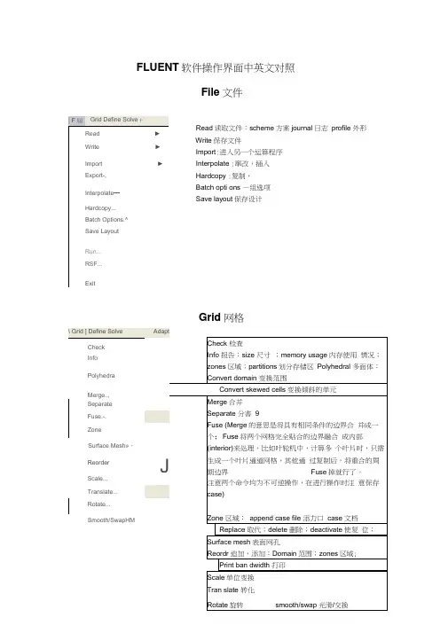
FLUENT 软件操作界面中英文对照File 文件Read 读取文件：scheme 方案journal 日志 profile 外形 Write 保存文件 Import :进入另一个运算程序 Interpolate :窜改，插入Hardcopy :复制，Batch opti ons —组选项Save layout 保存设计 Grid 网格| F 屆 Grid Define Solve i-Read► Write►Import ► Export-, Interpolate —Hardcopy...Batch Options.^Save LayoutRun...RSF...ExitDefine Models模型：solver解算器Pressure based 基于压力Den sity based基于密度末解用丁 pressure based,雀改用Censity based 岀观不苻合秦相36的摄不，请甸pres 羊WE base d Al density based 慎仆则迢.41刊卜 IS 况？北外.血OC ・EHU ^ cotipled ＞（/^ ptiaw ccupl ed simple 可这孔 & pimple ijEpiso 逞划.--■轟=Sortg 冲-丸布时制* ^jfe-5-6 1844DOden ba&ed 亘工F 吋.压聲血ptessurt ba$«i 适可于那可乐册斤"dens Ply based 把丸“河悴掏t ：至殳嗟之一.刑牛可爪門d 的创R 监當歎1一，般如人锻暮叫人丄有用 轴怀，火薩墟迭牛才H5）-0 程：yje8D8-丸布门 1叫；20GS-3-7 10-2ODQ歆；I ：谢PrflSsdrfl-Bawd Soker ^Fluflnt 它星英于压力快的束解孤便丹的圮压力修止畀法"求释旳控制片悝足标联式的，擅K 家鮮不町压縮舐Mb 对于町压砂也可旦索麟；Fk«nl 6-3 tl 前的I 板』冷孵臥 B fjS4^r«^at«d &Olvar fli Cfruptod Solvtr,的实也fltje Pr#4iurft-ea5<KJ ScFvAi 约两种虽幵方ib应理拈Fluent 氐J 眇坝犢型小的.它拈垒于曲喪红旳求聲塞，最辑的出H .也桿 艮先■那式的.丰誓■載密式冇Roz AU$hk>谏方法的初和&让Fhwrt 耳有比我甘的求IT 可压胃（说 劫謹力，們耳帕榕式淮冇琴加IF 科限闾辉，倒比还丰A 完荐匚Coupted 的算送t 对子慨站何Hh 地们足便用円匕口讷油皿购 加£未处為 性上世魅端计棒低逢刈趾.擁说的DansJty-Bjiwd Solver F ft St SiMPLEC, P 怡DE 些选以的.闪为進些ffliQl ；力修止鼻袪・不金在这种类崖的我押■中氏现泊I 建址祢匹足整用Fw»ur 护P.sed Solver 堺决昧的利底*implicit 隐式， explicit 显示Space 空间：2D , axisymmetric （转动轴）， axisymmetric swirl （漩涡转动轴）；Time 时间 :steady 定常，unsteady 非定常 Velocity formulatio n 制定速度： absolute 绝对的；relative 相对的Gradient option 梯度选择：以单元作基础；以节点作基础；以单元作梯度的最小正方形。

Support vector machine:A tool for mapping mineral prospectivityRenguang Zuo a,n,Emmanuel John M.Carranza ba State Key Laboratory of Geological Processes and Mineral Resources,China University of Geosciences,Wuhan430074;Beijing100083,Chinab Department of Earth Systems Analysis,Faculty of Geo-Information Science and Earth Observation(ITC),University of Twente,Enschede,The Netherlandsa r t i c l e i n f oArticle history:Received17May2010Received in revised form3September2010Accepted25September2010Keywords:Supervised learning algorithmsKernel functionsWeights-of-evidenceTurbidite-hosted AuMeguma Terraina b s t r a c tIn this contribution,we describe an application of support vector machine(SVM),a supervised learningalgorithm,to mineral prospectivity mapping.The free R package e1071is used to construct a SVM withsigmoid kernel function to map prospectivity for Au deposits in western Meguma Terrain of Nova Scotia(Canada).The SVM classification accuracies of‘deposit’are100%,and the SVM classification accuracies ofthe‘non-deposit’are greater than85%.The SVM classifications of mineral prospectivity have5–9%lowertotal errors,13–14%higher false-positive errors and25–30%lower false-negative errors compared tothose of the WofE prediction.The prospective target areas predicted by both SVM and WofE reflect,nonetheless,controls of Au deposit occurrence in the study area by NE–SW trending anticlines andcontact zones between Goldenville and Halifax Formations.The results of the study indicate theusefulness of SVM as a tool for predictive mapping of mineral prospectivity.&2010Elsevier Ltd.All rights reserved.1.IntroductionMapping of mineral prospectivity is crucial in mineral resourcesexploration and mining.It involves integration of information fromdiverse geoscience datasets including geological data(e.g.,geologicalmap),geochemical data(e.g.,stream sediment geochemical data),geophysical data(e.g.,magnetic data)and remote sensing data(e.g.,multispectral satellite data).These sorts of data can be visualized,processed and analyzed with the support of computer and GIStechniques.Geocomputational techniques for mapping mineral pro-spectivity include weights of evidence(WofE)(Bonham-Carter et al.,1989),fuzzy WofE(Cheng and Agterberg,1999),logistic regression(Agterberg and Bonham-Carter,1999),fuzzy logic(FL)(Ping et al.,1991),evidential belief functions(EBF)(An et al.,1992;Carranza andHale,2003;Carranza et al.,2005),neural networks(NN)(Singer andKouda,1996;Porwal et al.,2003,2004),a‘wildcat’method(Carranza,2008,2010;Carranza and Hale,2002)and a hybrid method(e.g.,Porwalet al.,2006;Zuo et al.,2009).These techniques have been developed toquantify indices of occurrence of mineral deposit occurrence byintegrating multiple evidence layers.Some geocomputational techni-ques can be performed using popular software packages,such asArcWofE(a free ArcView extension)(Kemp et al.,1999),ArcSDM9.3(afree ArcGIS9.3extension)(Sawatzky et al.,2009),MI-SDM2.50(aMapInfo extension)(Avantra Geosystems,2006),GeoDAS(developedbased on MapObjects,which is an Environmental Research InstituteDevelopment Kit)(Cheng,2000).Other geocomputational techniques(e.g.,FL and NN)can be performed by using R and Matlab.Geocomputational techniques for mineral prospectivity map-ping can be categorized generally into two types–knowledge-driven and data-driven–according to the type of inferencemechanism considered(Bonham-Carter1994;Pan and Harris2000;Carranza2008).Knowledge-driven techniques,such as thosethat apply FL and EBF,are based on expert knowledge andexperience about spatial associations between mineral prospec-tivity criteria and mineral deposits of the type sought.On the otherhand,data-driven techniques,such as WofE and NN,are based onthe quantification of spatial associations between mineral pro-spectivity criteria and known occurrences of mineral deposits ofthe type sought.Additional,the mixing of knowledge-driven anddata-driven methods also is used for mapping of mineral prospec-tivity(e.g.,Porwal et al.,2006;Zuo et al.,2009).Every geocomputa-tional technique has advantages and disadvantages,and one or theother may be more appropriate for a given geologic environmentand exploration scenario(Harris et al.,2001).For example,one ofthe advantages of WofE is its simplicity,and straightforwardinterpretation of the weights(Pan and Harris,2000),but thismodel ignores the effects of possible correlations amongst inputpredictor patterns,which generally leads to biased prospectivitymaps by assuming conditional independence(Porwal et al.,2010).Comparisons between WofE and NN,NN and LR,WofE,NN and LRfor mineral prospectivity mapping can be found in Singer andKouda(1999),Harris and Pan(1999)and Harris et al.(2003),respectively.Mapping of mineral prospectivity is a classification process,because its product(i.e.,index of mineral deposit occurrence)forevery location is classified as either prospective or non-prospectiveaccording to certain combinations of weighted mineral prospec-tivity criteria.There are two types of classification techniques.Contents lists available at ScienceDirectjournal homepage:/locate/cageoComputers&Geosciences0098-3004/$-see front matter&2010Elsevier Ltd.All rights reserved.doi:10.1016/j.cageo.2010.09.014n Corresponding author.E-mail addresses:zrguang@,zrguang1981@(R.Zuo).Computers&Geosciences](]]]])]]]–]]]One type is known as supervised classification,which classifies mineral prospectivity of every location based on a training set of locations of known deposits and non-deposits and a set of evidential data layers.The other type is known as unsupervised classification, which classifies mineral prospectivity of every location based solely on feature statistics of individual evidential data layers.A support vector machine(SVM)is a model of algorithms for supervised classification(Vapnik,1995).Certain types of SVMs have been developed and applied successfully to text categorization, handwriting recognition,gene-function prediction,remote sensing classification and other studies(e.g.,Joachims1998;Huang et al.,2002;Cristianini and Scholkopf,2002;Guo et al.,2005; Kavzoglu and Colkesen,2009).An SVM performs classification by constructing an n-dimensional hyperplane in feature space that optimally separates evidential data of a predictor variable into two categories.In the parlance of SVM literature,a predictor variable is called an attribute whereas a transformed attribute that is used to define the hyperplane is called a feature.The task of choosing the most suitable representation of the target variable(e.g.,mineral prospectivity)is known as feature selection.A set of features that describes one case(i.e.,a row of predictor values)is called a feature vector.The feature vectors near the hyperplane are the support feature vectors.The goal of SVM modeling is tofind the optimal hyperplane that separates clusters of feature vectors in such a way that feature vectors representing one category of the target variable (e.g.,prospective)are on one side of the plane and feature vectors representing the other category of the target variable(e.g.,non-prospective)are on the other size of the plane.A good separation is achieved by the hyperplane that has the largest distance to the neighboring data points of both categories,since in general the larger the margin the better the generalization error of the classifier.In this paper,SVM is demonstrated as an alternative tool for integrating multiple evidential variables to map mineral prospectivity.2.Support vector machine algorithmsSupport vector machines are supervised learning algorithms, which are considered as heuristic algorithms,based on statistical learning theory(Vapnik,1995).The classical task of a SVM is binary (two-class)classification.Suppose we have a training set composed of l feature vectors x i A R n,where i(¼1,2,y,n)is the number of feature vectors in training samples.The class in which each sample is identified to belong is labeled y i,which is equal to1for one class or is equal toÀ1for the other class(i.e.y i A{À1,1})(Huang et al., 2002).If the two classes are linearly separable,then there exists a family of linear separators,also called separating hyperplanes, which satisfy the following set of equations(KavzogluandFig.1.Support vectors and optimum hyperplane for the binary case of linearly separable data sets.Table1Experimental data.yer A Layer B Layer C Layer D Target yer A Layer B Layer C Layer D Target1111112100000 2111112200000 3111112300000 4111112401000 5111112510000 6111112600000 7111112711100 8111112800000 9111012900000 10111013000000 11101113111100 12111013200000 13111013300000 14111013400000 15011013510000 16101013600000 17011013700000 18010113811100 19010112900000 20101014010000R.Zuo,E.J.M.Carranza/Computers&Geosciences](]]]])]]]–]]]2Colkesen,2009)(Fig.1):wx iþb Zþ1for y i¼þ1wx iþb rÀ1for y i¼À1ð1Þwhich is equivalent toy iðwx iþbÞZ1,i¼1,2,...,nð2ÞThe separating hyperplane can then be formalized as a decision functionfðxÞ¼sgnðwxþbÞð3Þwhere,sgn is a sign function,which is defined as follows:sgnðxÞ¼1,if x400,if x¼0À1,if x o08><>:ð4ÞThe two parameters of the separating hyperplane decision func-tion,w and b,can be obtained by solving the following optimization function:Minimize tðwÞ¼12J w J2ð5Þsubject toy Iððwx iÞþbÞZ1,i¼1,...,lð6ÞThe solution to this optimization problem is the saddle point of the Lagrange functionLðw,b,aÞ¼1J w J2ÀX li¼1a iðy iððx i wÞþbÞÀ1Þð7Þ@ @b Lðw,b,aÞ¼0@@wLðw,b,aÞ¼0ð8Þwhere a i is a Lagrange multiplier.The Lagrange function is minimized with respect to w and b and is maximized with respect to a grange multipliers a i are determined by the following optimization function:MaximizeX li¼1a iÀ12X li,j¼1a i a j y i y jðx i x jÞð9Þsubject toa i Z0,i¼1,...,l,andX li¼1a i y i¼0ð10ÞThe separating rule,based on the optimal hyperplane,is the following decision function:fðxÞ¼sgnX li¼1y i a iðxx iÞþb!ð11ÞMore details about SVM algorithms can be found in Vapnik(1995) and Tax and Duin(1999).3.Experiments with kernel functionsFor spatial geocomputational analysis of mineral exploration targets,the decision function in Eq.(3)is a kernel function.The choice of a kernel function(K)and its parameters for an SVM are crucial for obtaining good results.The kernel function can be usedTable2Errors of SVM classification using linear kernel functions.l Number ofsupportvectors Testingerror(non-deposit)(%)Testingerror(deposit)(%)Total error(%)0.2580.00.00.0180.00.00.0 1080.00.00.0 10080.00.00.0 100080.00.00.0Table3Errors of SVM classification using polynomial kernel functions when d¼3and r¼0. l Number ofsupportvectorsTestingerror(non-deposit)(%)Testingerror(deposit)(%)Total error(%)0.25120.00.00.0160.00.00.01060.00.00.010060.00.00.0 100060.00.00.0Table4Errors of SVM classification using polynomial kernel functions when l¼0.25,r¼0.d Number ofsupportvectorsTestingerror(non-deposit)(%)Testingerror(deposit)(%)Total error(%)11110.00.0 5.010290.00.00.0100230.045.022.5 1000200.090.045.0Table5Errors of SVM classification using polynomial kernel functions when l¼0.25and d¼3.r Number ofsupportvectorsTestingerror(non-deposit)(%)Testingerror(deposit)(%)Total error(%)0120.00.00.01100.00.00.01080.00.00.010080.00.00.0 100080.00.00.0Table6Errors of SVM classification using radial kernel functions.l Number ofsupportvectorsTestingerror(non-deposit)(%)Testingerror(deposit)(%)Total error(%)0.25140.00.00.01130.00.00.010130.00.00.0100130.00.00.0 1000130.00.00.0Table7Errors of SVM classification using sigmoid kernel functions when r¼0.l Number ofsupportvectorsTestingerror(non-deposit)(%)Testingerror(deposit)(%)Total error(%)0.25400.00.00.01400.035.017.510400.0 6.0 3.0100400.0 6.0 3.0 1000400.0 6.0 3.0R.Zuo,E.J.M.Carranza/Computers&Geosciences](]]]])]]]–]]]3to construct a non-linear decision boundary and to avoid expensive calculation of dot products in high-dimensional feature space.The four popular kernel functions are as follows:Linear:Kðx i,x jÞ¼l x i x j Polynomial of degree d:Kðx i,x jÞ¼ðl x i x jþrÞd,l40Radial basis functionðRBFÞ:Kðx i,x jÞ¼exp fÀl99x iÀx j992g,l40 Sigmoid:Kðx i,x jÞ¼tanhðl x i x jþrÞ,l40ð12ÞThe parameters l,r and d are referred to as kernel parameters. The parameter l serves as an inner product coefficient in the polynomial function.In the case of the RBF kernel(Eq.(12)),l determines the RBF width.In the sigmoid kernel,l serves as an inner product coefficient in the hyperbolic tangent function.The parameter r is used for kernels of polynomial and sigmoid types. The parameter d is the degree of a polynomial function.We performed some experiments to explore the performance of the parameters used in a kernel function.The dataset used in the experiments(Table1),which are derived from the study area(see below),were compiled according to the requirementfor Fig.2.Simplified geological map in western Meguma Terrain of Nova Scotia,Canada(after,Chatterjee1983;Cheng,2008).Table8Errors of SVM classification using sigmoid kernel functions when l¼0.25.r Number ofSupportVectorsTestingerror(non-deposit)(%)Testingerror(deposit)(%)Total error(%)0400.00.00.01400.00.00.010400.00.00.0100400.00.00.01000400.00.00.0R.Zuo,E.J.M.Carranza/Computers&Geosciences](]]]])]]]–]]]4classification analysis.The e1071(Dimitriadou et al.,2010),a freeware R package,was used to construct a SVM.In e1071,the default values of l,r and d are1/(number of variables),0and3,respectively.From the study area,we used40geological feature vectors of four geoscience variables and a target variable for classification of mineral prospec-tivity(Table1).The target feature vector is either the‘non-deposit’class(or0)or the‘deposit’class(or1)representing whether mineral exploration target is absent or present,respectively.For‘deposit’locations,we used the20known Au deposits.For‘non-deposit’locations,we randomly selected them according to the following four criteria(Carranza et al.,2008):(i)non-deposit locations,in contrast to deposit locations,which tend to cluster and are thus non-random, must be random so that multivariate spatial data signatures are highly non-coherent;(ii)random non-deposit locations should be distal to any deposit location,because non-deposit locations proximal to deposit locations are likely to have similar multivariate spatial data signatures as the deposit locations and thus preclude achievement of desired results;(iii)distal and random non-deposit locations must have values for all the univariate geoscience spatial data;(iv)the number of distal and random non-deposit locations must be equaltoFig.3.Evidence layers used in mapping prospectivity for Au deposits(from Cheng,2008):(a)and(b)represent optimum proximity to anticline axes(2.5km)and contacts between Goldenville and Halifax formations(4km),respectively;(c)and(d)represent,respectively,background and anomaly maps obtained via S-Afiltering of thefirst principal component of As,Cu,Pb and Zn data.R.Zuo,E.J.M.Carranza/Computers&Geosciences](]]]])]]]–]]]5the number of deposit locations.We used point pattern analysis (Diggle,1983;2003;Boots and Getis,1988)to evaluate degrees of spatial randomness of sets of non-deposit locations and tofind distance from any deposit location and corresponding probability that one deposit location is situated next to another deposit location.In the study area,we found that the farthest distance between pairs of Au deposits is71km,indicating that within that distance from any deposit location in there is100%probability of another deposit location. However,few non-deposit locations can be selected beyond71km of the individual Au deposits in the study area.Instead,we selected random non-deposit locations beyond11km from any deposit location because within this distance from any deposit location there is90% probability of another deposit location.When using a linear kernel function and varying l from0.25to 1000,the number of support vectors and the testing errors for both ‘deposit’and‘non-deposit’do not vary(Table2).In this experiment the total error of classification is0.0%,indicating that the accuracy of classification is not sensitive to the choice of l.With a polynomial kernel function,we tested different values of l, d and r as follows.If d¼3,r¼0and l is increased from0.25to1000,the number of support vectors decreases from12to6,but the testing errors for‘deposit’and‘non-deposit’remain nil(Table3).If l¼0.25, r¼0and d is increased from1to1000,the number of support vectors firstly increases from11to29,then decreases from23to20,the testing error for‘non-deposit’decreases from10.0%to0.0%,whereas the testing error for‘deposit’increases from0.0%to90%(Table4). In this experiment,the total error of classification is minimum(0.0%) when d¼10(Table4).If l¼0.25,d¼3and r is increased from 0to1000,the number of support vectors decreases from12to8,but the testing errors for‘deposit’and‘non-deposit’remain nil(Table5).When using a radial kernel function and varying l from0.25to 1000,the number of support vectors decreases from14to13,but the testing errors of‘deposit’and‘non-deposit’remain nil(Table6).With a sigmoid kernel function,we experimented with different values of l and r as follows.If r¼0and l is increased from0.25to1000, the number of support vectors is40,the testing errors for‘non-deposit’do not change,but the testing error of‘deposit’increases from 0.0%to35.0%,then decreases to6.0%(Table7).In this experiment,the total error of classification is minimum at0.0%when l¼0.25 (Table7).If l¼0.25and r is increased from0to1000,the numbers of support vectors and the testing errors of‘deposit’and‘non-deposit’do not change and the total error remains nil(Table8).The results of the experiments demonstrate that,for the datasets in the study area,a linear kernel function,a polynomial kernel function with d¼3and r¼0,or l¼0.25,r¼0and d¼10,or l¼0.25and d¼3,a radial kernel function,and a sigmoid kernel function with r¼0and l¼0.25are optimal kernel functions.That is because the testing errors for‘deposit’and‘non-deposit’are0%in the SVM classifications(Tables2–8).Nevertheless,a sigmoid kernel with l¼0.25and r¼0,compared to all the other kernel functions,is the most optimal kernel function because it uses all the input support vectors for either‘deposit’or‘non-deposit’(Table1)and the training and testing errors for‘deposit’and‘non-deposit’are0% in the SVM classification(Tables7and8).4.Prospectivity mapping in the study areaThe study area is located in western Meguma Terrain of Nova Scotia,Canada.It measures about7780km2.The host rock of Au deposits in this area consists of Cambro-Ordovician low-middle grade metamorphosed sedimentary rocks and a suite of Devonian aluminous granitoid intrusions(Sangster,1990;Ryan and Ramsay, 1997).The metamorphosed sedimentary strata of the Meguma Group are the lower sand-dominatedflysch Goldenville Formation and the upper shalyflysch Halifax Formation occurring in the central part of the study area.The igneous rocks occur mostly in the northern part of the study area(Fig.2).In this area,20turbidite-hosted Au deposits and occurrences (Ryan and Ramsay,1997)are found in the Meguma Group, especially near the contact zones between Goldenville and Halifax Formations(Chatterjee,1983).The major Au mineralization-related geological features are the contact zones between Gold-enville and Halifax Formations,NE–SW trending anticline axes and NE–SW trending shear zones(Sangster,1990;Ryan and Ramsay, 1997).This dataset has been used to test many mineral prospec-tivity mapping algorithms(e.g.,Agterberg,1989;Cheng,2008). More details about the geological settings and datasets in this area can be found in Xu and Cheng(2001).We used four evidence layers(Fig.3)derived and used by Cheng (2008)for mapping prospectivity for Au deposits in the yers A and B represent optimum proximity to anticline axes(2.5km) and optimum proximity to contacts between Goldenville and Halifax Formations(4km),yers C and D represent variations in geochemical background and anomaly,respectively, as modeled by multifractalfilter mapping of thefirst principal component of As,Cu,Pb,and Zn data.Details of how the four evidence layers were obtained can be found in Cheng(2008).4.1.Training datasetThe application of SVM requires two subsets of training loca-tions:one training subset of‘deposit’locations representing presence of mineral deposits,and a training subset of‘non-deposit’locations representing absence of mineral deposits.The value of y i is1for‘deposits’andÀ1for‘non-deposits’.For‘deposit’locations, we used the20known Au deposits(the sixth column of Table1).For ‘non-deposit’locations(last column of Table1),we obtained two ‘non-deposit’datasets(Tables9and10)according to the above-described selection criteria(Carranza et al.,2008).We combined the‘deposits’dataset with each of the two‘non-deposit’datasets to obtain two training datasets.Each training dataset commonly contains20known Au deposits but contains different20randomly selected non-deposits(Fig.4).4.2.Application of SVMBy using the software e1071,separate SVMs both with sigmoid kernel with l¼0.25and r¼0were constructed using the twoTable9The value of each evidence layer occurring in‘non-deposit’dataset1.yer A Layer B Layer C Layer D100002000031110400005000061000700008000090100 100100 110000 120000 130000 140000 150000 160100 170000 180000 190100 200000R.Zuo,E.J.M.Carranza/Computers&Geosciences](]]]])]]]–]]] 6training datasets.With training dataset1,the classification accuracies for‘non-deposits’and‘deposits’are95%and100%, respectively;With training dataset2,the classification accuracies for‘non-deposits’and‘deposits’are85%and100%,respectively.The total classification accuracies using the two training datasets are97.5%and92.5%,respectively.The patterns of the predicted prospective target areas for Au deposits(Fig.5)are defined mainly by proximity to NE–SW trending anticlines and proximity to contact zones between Goldenville and Halifax Formations.This indicates that‘geology’is better than‘geochemistry’as evidence of prospectivity for Au deposits in this area.With training dataset1,the predicted prospective target areas occupy32.6%of the study area and contain100%of the known Au deposits(Fig.5a).With training dataset2,the predicted prospec-tive target areas occupy33.3%of the study area and contain95.0% of the known Au deposits(Fig.5b).In contrast,using the same datasets,the prospective target areas predicted via WofE occupy 19.3%of study area and contain70.0%of the known Au deposits (Cheng,2008).The error matrices for two SVM classifications show that the type1(false-positive)and type2(false-negative)errors based on training dataset1(Table11)and training dataset2(Table12)are 32.6%and0%,and33.3%and5%,respectively.The total errors for two SVM classifications are16.3%and19.15%based on training datasets1and2,respectively.In contrast,the type1and type2 errors for the WofE prediction are19.3%and30%(Table13), respectively,and the total error for the WofE prediction is24.65%.The results show that the total errors of the SVM classifications are5–9%lower than the total error of the WofE prediction.The 13–14%higher false-positive errors of the SVM classifications compared to that of the WofE prediction suggest that theSVMFig.4.The locations of‘deposit’and‘non-deposit’.Table10The value of each evidence layer occurring in‘non-deposit’dataset2.yer A Layer B Layer C Layer D110102000030000411105000060110710108000091000101110111000120010131000140000150000161000171000180010190010200000R.Zuo,E.J.M.Carranza/Computers&Geosciences](]]]])]]]–]]]7classifications result in larger prospective areas that may not contain undiscovered deposits.However,the 25–30%higher false-negative error of the WofE prediction compared to those of the SVM classifications suggest that the WofE analysis results in larger non-prospective areas that may contain undiscovered deposits.Certainly,in mineral exploration the intentions are notto miss undiscovered deposits (i.e.,avoid false-negative error)and to minimize exploration cost in areas that may not really contain undiscovered deposits (i.e.,keep false-positive error as low as possible).Thus,results suggest the superiority of the SVM classi-fications over the WofE prediction.5.ConclusionsNowadays,SVMs have become a popular geocomputational tool for spatial analysis.In this paper,we used an SVM algorithm to integrate multiple variables for mineral prospectivity mapping.The results obtained by two SVM applications demonstrate that prospective target areas for Au deposits are defined mainly by proximity to NE–SW trending anticlines and to contact zones between the Goldenville and Halifax Formations.In the study area,the SVM classifications of mineral prospectivity have 5–9%lower total errors,13–14%higher false-positive errors and 25–30%lower false-negative errors compared to those of the WofE prediction.These results indicate that SVM is a potentially useful tool for integrating multiple evidence layers in mineral prospectivity mapping.Table 11Error matrix for SVM classification using training dataset 1.Known All ‘deposits’All ‘non-deposits’TotalPrediction ‘Deposit’10032.6132.6‘Non-deposit’067.467.4Total100100200Type 1(false-positive)error ¼32.6.Type 2(false-negative)error ¼0.Total error ¼16.3.Note :Values in the matrix are percentages of ‘deposit’and ‘non-deposit’locations.Table 12Error matrix for SVM classification using training dataset 2.Known All ‘deposits’All ‘non-deposits’TotalPrediction ‘Deposits’9533.3128.3‘Non-deposits’566.771.4Total100100200Type 1(false-positive)error ¼33.3.Type 2(false-negative)error ¼5.Total error ¼19.15.Note :Values in the matrix are percentages of ‘deposit’and ‘non-deposit’locations.Table 13Error matrix for WofE prediction.Known All ‘deposits’All ‘non-deposits’TotalPrediction ‘Deposit’7019.389.3‘Non-deposit’3080.7110.7Total100100200Type 1(false-positive)error ¼19.3.Type 2(false-negative)error ¼30.Total error ¼24.65.Note :Values in the matrix are percentages of ‘deposit’and ‘non-deposit’locations.Fig.5.Prospective targets area for Au deposits delineated by SVM.(a)and (b)are obtained using training dataset 1and 2,respectively.R.Zuo,E.J.M.Carranza /Computers &Geosciences ](]]]])]]]–]]]8。

SOPA：Source Routing Based PacketLevel MultiPath Routingin Data Center NetworksMany “rich?connected”topologies with multiple parallel paths between servers have been proposed for data center networks recently to provide high bisection bandwidth，but it remains challenging to fully utilize the high network capacity by appropriate multi?path routing algorithms. As flow?level path splitting may lead to traffic imbalance between paths due to flow size difference，packet?level path splitting attracts more attention lately，which spreads packets from flows into multiple available paths and significantly improves link utilizations. However，it may cause packet reordering，confusing the TCP congestion control algorithm and lowering the throughput of flows. In this paper，we design a novel packet?level multi?path routing scheme called SOPA，which leverages OpenFlow to perform packet?level path splitting in a round?robin fashion，and hence significantly mitigates the packet reordering problem and improves the network throughput. Moreover，SOPA leverages the topological feature of data center networks to encode a very small number of switches along the path into the packet header，resulting in very lightoverhead. Compared with random packet spraying （RPS），Hedera and equal?cost multi?path routing （ECMP），our simulations demonstrate that SOPA achieves 29.87%，50.41% and 77.74% higher network throughput respectively under permutation workload，and reduces average data transfer completion time by 53.65%，343.31% and 348.25% respectively under production workload.data center networks；multi?path routing；path splitting Keywords1 Introductionata center networks connect hundred of thousands of servers to support cloud computing，including both front?end online services （e.g.，web search and gaming）and back?end distributed computations （e.g.，distributed file system [1] and distributed data processing engine [2]，[3]）. Recognizing that the traditional tree?based topology cannot well embrace the bandwidth?hungry cloud services，in recent years many “rich?connected”data center network topologies have been proposed，such as Fat?Tree [4]，VL2 [5]，BCube [6] and FiConn [7]. These new topologies provide multiple paths between any pair of servers，and greatly increase the network bisection bandwidth. For instance，in a Fat?Tree network，there are x equal paths between two servers from different pods，where x is the number of core switches in the network；while in a [BCuben，k] network，[k+1]non?disjoint paths exist between any two servers，not to mention the paths with overlapping links. Although the advanced data center networks enjoy high network capacity，it remains challenging how to fully utilize the capacity and provide high network throughput to upper?layer applications. Multi?path routing is necessary to exploit the abundant paths between servers. The existing multi?path routing schemes can be divided into two categories，namely，flow?level path splitting and packet?level path splitting. In flow?level path splitting solutions，traffic between two servers is split into different paths at the flow granularity.All the packets belonging to a 5?tuple flow traverse the same path，so as to avoid out?of?order delivery. For examples，equal?cost multi?path routing （ECMP）uses 5?tuple hashing to choose the path for a flow from the multiple candidates，with the possibility of hash collision and unequal utilization of the paths；in order to avoid the hash collision between large flows，Hedera [8] explores a centralized way to schedule the flows by spreading large flows into different paths. However，the flow sizes and packet sizes of different flows are usually diversified，which can also lead to traffic imbalance among different paths.Packet?level path splitting，on the other hand，splits traffic in the packet granularity，i.e.，packets from a flow can be put to different paths. Since packets of the same flow are usually of similar sizes，packet?level path splitting achieves desirable traffic balance among multiple candidate paths. However，a major concern of packet?level path splitting is that it may cause packet reordering for TCP flows. Although recent studies showed that the path equivalence in modern data center networks can help mitigate the packet reordering problem，random next?hop selection in random packet spraying （RPS）[9] still results in considerable packet reordering and unsatisfactory flow throughputs，which is worsen when link fails and network symmetry is broken [9]. DRB [10] employs IP?in?IP encapsulation/decapsulation [11] to select the core level switch and uses re?sequencing buffer at the receiver to absorb reordered packets，which not only introduces much traffic overhead，but also causes considerable re?sequencing delay [10].In this paper we design SOPA，a new packet?level path splitting scheme to carry on multi?path routing in data center networks. SOPA advances the state of art by two technicalinnovations.First，rather than introducing an additional buffer at the receiver，SOPA increases the fast retransmit （FR）threshold （i.e.，the number of duplicate ACKs received at the sender that acknowledge the same sequence number）used in TCP to trigger FR，so as to mitigate the impact of packet reordering on reducing flow’s throughput. In the current TCP congestion control algorithm，packet reordering is regarded as an indicator of packet loss，hence three duplicate ACKs will cause packet retransmit at the sender without waiting for the timeouts. Although it works well in single?path routing，in multi?path routing paradigm it misleads the congestion control algorithm，since in most cases packet reordering does not come from packet loss. By increasing the FR threshold，say，to 10，SOPA significantly reduces the number of unnecessary packet retransmits，which accordingly improves the effective throughput for a flow. Fig. 11 shows the Cumulative Distribution Function （CDF）of all the flows’throughput. We can see that SOPA significantly outperforms the other three multi?path routing schemes. The average throughput of SOPA is 925.13 Mbit/s，and all the flows’throughputs are above 910 Mbit/s. Compared with SOPA，the average throughput of theflows drops by 47.47% in RPS. The fundamental reason is as explained above：RPS cannot evenly split the traffic across candidate paths，and unequal queue lengths will be built. So the receivers will receive more reordered packets，and unnecessary FRs will be triggered at the senders. As flow?based path splitting solutions，Hedera and ECMP expose even lower performance than RPS. Compared with SOPA，the average throughput drops by 75.21% and 76.48%，respectively. The basic reason is that the flow?based multi?path routing cannot fully utilize the rich link resource in the Fat?Tree network. ECMP achieves the lowest throughput because the hashing results of some flows may collide and be scheduled to the same path，which can be avoided by centralized negotiation in Hedera.4.4 Production WorkloadWe next study the performance under a more realistic workloads from a production data center [5]：95% flows are less than 1 MB，and only less than 2% flows exceeds 10 MB. Different from the permutation workload，in this simulation the data is transmitted by multiple flows instead of a single one. The flows are issued sequentially，and each flow randomly picks a destination server. All the servers start data transmission at thesame time，and we measure the average throughput of the data transmission under this workload.In our simulation，the average throughput for SOPA，RPS，Hedera，and ECMP are 465.5 Mbit/s，302.96 Mbit/s，105.005 Mbit/s，and 103.849 Mbit/s，respectively. ECMP gets the lowest throughput，since it neither evenly spreads the flows into multiple paths nor considers traffic sizes in splitting. Hedera performs a little better than ECMP，but the gap is marginal （less than 2 Mbit/s）. It is because Hedera targets at scheduling large flows but in this workload 95% flows are small ones （with data size less than 1 MB）. Both RPS and SOPA can achieve much higher throughput，due to the fine?grained link utilization by packet?level path splitting. Compared with RPS，SOPA can even improve the throughput by 53.65%，since it explicitly spreads the traffic into the multiple paths in a more balanced way. The result is consistent with that in previous simulations. 4.5 Link FailuresWe then evaluate the performance of SOPA when failure occurs. Since failure brings more negative effect forpacket?level traffic splitting （introducing more aggravated packet reordering），we only compare SOPA with RPS in this group of simulations. We use production workload to conductsimulation in the same topology as that in the previous simulation. We let the leftmost aggregation switch in the first Pod break down. Fig. 12 shows the result. In order to showcase the effect of failure，the performance without failure is also plotted.The x?axis of Fig. 12 denotes both multi?path routing schemes under different settings，wherein “NF”in parenthesis means no failure，and “F”in parenthesis denotes failures. The y?axis shows the throughput of flows. Similarly，for each candlestick in the figure，the top and bottom of the straight line represent the maximum and minimum values of the flow’s throughput，respectively. The top and bottom of the rectangle denote the 5th and 99th percentile of average throughput，respectively. The short black line is the average throughput of all flows.The performance of SOPA is almost not affected by the link failure at all，and only the minimum throughput decreases from 244 Mbit/s to 188.17 Mbit/s. This mild performance degradation is attributed to the high FR threshold of SOPA，which can absorb the more reordered packets introduced by the failure. However，failure brings more negative effects to RPS，and both the maximum and minimum throughput of RPS aredropped. When there is no failure，the maximum and minimum throughput are 865.41 Mbit/s and 214.54 Mbit/s，respectively. But in the failure case，their values drop to 672.25 Mbit/s and 26.17 Mbit/s，respectively. This performance degradation is primarily caused by timeouts of the retransmission timers. Trace data shows that when failure occurs，RPS experiences 67 times of timeout and 12000 packets have been dropped （as a contract，there is no packet loss when no failure）. The packet losses are caused by traffic congestion，since RPS cannot achieve balanced traffic splitting and the failure aggravates this situation. However，benefiting from balanced traffic splitting，SOPA does not cause packet loss，and there is not a single timeout in the simulation，with or without failures.5 ConclusionMany “rich?connected”topologies have been proposed for data centers in recently years，such as Fat?Tree，to provide full bisection bandwidth. To achieve high aggregate bandwidth，the flows need to dynamically choose a path or simultaneously transmit data on multiple paths. Existing flow?level multipath routing solutions do not consider the data size，and may lead to traffic imbalance. While the packet?level multipath routing scheme may create large queue length differential betweencandidate paths，aggravating packet reordering at receivers and thus triggering FR at the senders. In this paper we design SOPA to efficiently utilize the high network capacity. SOPA adopts source routing to explicitly split data to candidate routing paths in a round robin fashion，which can significantly mitigate packet reordering and thus improve the network throughput. By leveraging the topological feature of data center networks，SOPA encodes a very small number of switches into the packet header，introducing a very light overhead. SOPA also immediately throttles the transmission rate of the affected flow as soon as the failures are detected to promptly mitigate the negative affect of failures. NS?3 based simulations show SOPA can efficiently increase the network throughput，and outperform other schemes under different settings，irrespective of the network size. Reference[1] S. Ghemawat，H. Gobioff，and S.?T. Leung，“The google file system，”in Proc. 19th ACM Symposium on Operating Systems Principles，New York，USA，2003，pp. 29-43.[2] J. Dean and S. Ghemawat，“MapReduce：simplified data processing on large clusters，”in Proc. 6th Symposium on Operating Systems Design and Implementation，Berkeley，USA，2004，pp. 137-149.[3] M. Isard，M. Budiu，Y. Yu， A. Birrell，and D. Fetterly，“Dryad：distributed data?parallel programs from sequential building blocks，”in Proc. 2nd ACMSIGOPS/EuroSys European Conference on Computer Systems，New York，USA，2007，pp. 59-72. doi：10.1145/1272998.1273005.[4] M. Al?Fares，A. Loukissas，and A. Vahdat，“A scalable，commodity data center network architecture，”in Proc. ACM SIGCOMM 2008 Conference on Data Communication，Seattle，USA，2008，pp. 63-74. doi：10.1145/1402958. 1402967.[5] A. Greenberg，J. R. Hamilton，N. Jain，et al.，“VL2：a scalable and flexible data center network，”in Proc. ACM SIGCOMM 2009 Conference on Data Communication，Barcelona，Spain，2009，pp. 51-62. doi：10.1145/1592568. 1592576.[6] C. Guo，G. Lu，D. Li，et al.，“BCube：a high performance，server?centric network architecture for modular data centers，”in Proc. ACM SIGCOMM，Barcelona，Spain，2009，pp. 63-74.[7] D. Li， C. Guo，H. Wu，et al.，“Scalable andcost?effective interconnection of data?center servers using dual server ports，”IEEE/ACM Transactions on Networking，vol. 19，no. 1，pp. 102-114，Feb. 2011. doi：10.1109/TNET.2010.2053718.[8] M. Al?Fares，S. Radhakrishnan，B. Raghavan，N. Huang，and A. Vahdat，“Hedera：Dynamic flow scheduling for data center networks，”in Proc. 7th USENIX Symposium on Networked Systems Design and Implementation，San Jose，USA，2010，pp. 1-15.[9] A. Dixit，P. Prakash，Y. Hu，and R. Kompella，“On the impact of packet spraying in data center networks，”in Proc. IEEE INFOCOM，Turin，Italy，2013，pp. 2130-2138. doi：10.1109/INFCOM.2013.6567015.[10] J. Cao，R. Xia，P. Yang，et al.，“Per?packet load?balanced，low?latency routing for clos?based data center networks，”in Proc. Ninth ACM Conference on Emerging Networking Experiments and Technologies，Santa Barbara，USA，2013，pp. 49-60. doi：10.1145/2535372.2535375.[11] IETF. （2013，Mar. 2）. IP encapsulation within IP [Online]. Available：https：///doc/rfc2003[12] C. Guo，G. Lu，H. J. Wang，et al.，“Secondnet：a data center network virtualization architecture with bandwidthguarantees，”in Proc. 6th International Conference on Emerging Networking Experiments and Technologies，Philadelphia，USA，2010. doi：10.1145/1921168.1921188.[13] ONF. （2017，Apr. 1）. Open networking foundation [Online]. Available：https：//[14] A. Curtis，W. Kim，and P. Yalagandula，“Mahout：Low?overhead datacenter traffic management usingend?host?based elephant detection，”in Proc. IEEE INFOCOM，Shanghai，China，2011，pp. 1629-1637. doi：10.1109/INFCOM. 2011.5934956.[15] C. Raiciu，S. Barre，C. Pluntke，et al.，“Improving datacenter performance and robustness with multipath TCP，”in Proc. ACM SIGCOMM，Toronto，Canada，2011，pp. 266-277. doi：10.1145/2018436.2018467.[16] C. Raiciu，C. Paasch，S. Barr，et al.，“How hard can it be？Designing and implementing a deployable multipath TCP，”in USENIX Symposium of Networked Systems Design and Implementation，San Jose，USA，2012，pp. 29-29.[17] D. Wischik，C. Raiciu， A. Greenhalgh，and M. Handley，“Design，implementation and evaluation of congestion control for multipath TCP，”in Proc. 8th USENIX Conference on Networked Systems Design andImplementation，Boston，USA，2011，pp. 99-112.[18] M. Alizadeh，A. Greenberg，D. A. Maltz，et al.，“Data center TCP （DCTCP），”in Proc. ACM SIGCOMM，New York，USA，2010，pp. 63-74. doi：10.1145/1851182.1851192.[19] R. Niranjan Mysore， A. Pamboris，N. Farrington，et al.，“PortLand：a scalable fault?tolerant layer 2 data center network fabric，”in Proc. ACM SIGCOMM，Barcelona，Spain，2009，pp. 39-50. doi：10.1145/1594977.1592575.[20] NS?3 [Online]. Available：http：//Manuscript received：2017?03?22BiographiesLI Dan （tolidan@）received the M.E. degree and Ph.D. from Tsinghua University，China in 2005 and 2007 respectively，both in computer science. Before that，he spent four undergraduate years in Beijing Normal University，China and got a B.S. degree in 2003，also in computer science. He joined Microsoft Research Asia in Jan. 2008，where he worked as an associate researcher in Wireless and Networking Group until Feb. 2010. He joined the faculty of Tsinghua University in Mar. 2010，where he is now an associate professor at Computer Science Department. His researchinterests include Internet architecture and protocol design，data center network，and software defined networking.LIN Du （lindu1992@）received the B.S. degree from Tsinghua University，China in 2015. Now，he is a master candidate at the Department of Computer Science and Technology，Tsinghua University. His research interests include Internet architecture，data center network，and high?performance network system.JIANG Changlin（jiangchanglin@）received the B.S. and M.S. degrees from the Institute of Communication Engineering，PLA University of Science and Technology，China in 2001 and 2004 respectively. Now，he is a Ph.D. candidate at the Department of Computer Science and Technology，Tsinghua University，China. His research interests include Internet architecture，data center network，and network routing.WANG Lingqiang （wang.lingqiang@）received the B.S. degree from Department of Industrial Automation，Zhengzhou University，China in 1999. He is a system architect of ZTE Corporation. He focuses on technical planning and pre?research work in IP direction. His researchinterests include smart pipes，next generation broadband technology，and programmable networks.。

Quasiclassical trajectory calculations of collisional energy transfer in propane systemsApichart Linhananta and Kieran F.Lim*¤Centre for Chiral and Molecular T echnologies,School of Biological and Chemical Sciences,Deakin University,Geelong,V ictoria3217,Australia.E-mail:lim=.auRecei v ed6th December1999,Accepted27th January2000Published on the Web9th March2000Quasiclassical trajectory calculations of collisional energy transfer(CET)and rotational energy transfer from highly vibrationally excited propane to rare bath gases are reported.The calculations employed atomÈatom pairwise-additive Lennard-Jones,Buckingham exponential and hard-sphere intermolecular potentials to examine the dependence of CET on the intermolecular potential and to establish a protocol for future work on larger alkane systems.The role of the torsional(internal)and molecular(external)rotors in the energy-transfer mechanism were parison of the results with our earlier work on ethane]neon systems(A. Linhananta and K.F.Lim,Phys.Chem.Chem.Phys.,1999,1,3467)suggests that the internal and external rotors play a signiÐcant role in the deactivation mechanism for highly vibrationally excited alkanes.I.IntroductionGas-phase chemical reaction rates are strongly dependent on intermolecular collisional energy transfer(CET).CET is a vital component in any combustion-model and atmospheric-model systems.The only experimental CET quantities for hydrocarbon fuel molecules have been inferred““indirectlyÏÏfrom measurements of pressure-dependent reaction rates.1h3 Despite this,there have been no systematic theoretical dynamics studies of CET of hydrocarbon and halogenated hydrocarbons.In fact,most theoretical studies have been on small molecules.3h14The exceptions are the quasiclassical tra-jectory(QCT)calculations of azulene,toluene,benzene and hexaÑuorobenzene systems.15h23We have recently reported QCT calculations for highly vibrationally excited ethane in neon bath gas.24This and the recent work by Svedung et al. are,to our knowledge,theÐrst theoretical CET studies of an alkane with internal rotors.24,25Comparisons of theoretical and experimental studies of CET show that many of the dominant energy transfer mecha-nisms in small molecules are also present in large mol-ecules.3h6However,there are several di†erences between large-substrate and small-substrate behaviours.A notable example is that in the CET from a““smallÏÏsubstrate to a rare gas collider the trend He[Ne[Ar is observed,26h28 whereas the opposite trend of He\Ne\Ar is observed for ““largeÏÏsubstrates.29h39Theoretical studies of CET on small molecules employing various techniquesÈquantum,semi-classical and classical dynamicsÈall have correctly predicted the small-substrate behaviour.40,41This is not the case for large-substrate systems where QCT simulations incorrectly found the same smallsubstrate trend.15h18The discrepancy may be due to the lack of reliable data on the intermolecular potential surface involving large molecules and is most likely to be manifested in systems with the small collider helium bath gas.42,43¤Lim Pak Kwan.The aforementioned QCT calculations of large-substrate molecules have been on aromatic hydrocarbons because they have been most amenable to experimental studies using spec-troscopic probes.There have been fewer studies28,44h47on alkanes and branched-alkanes,which are the main com-ponents of common combustion fuels,and their halogenated analogues,which are important in ozone and““greenhouseÏÏchemistry.TheÐrst most obvious di†erences between alkanes and aromatics are their shapes,which are expected to a†ect the rotational energy transfer(RET).Since rotation to trans-lation(R]T)energy transfer and vibration to rotation (V]R)energy transfer are often more efficient than vibration to translation(V]T)energy transfer,this can have a strong inÑuence on the overall CET.Another crucial aspect is theÑexibility of alkanes.QCT simulations of alkanes would require the development of an efficient algorithm for sampling conformer space.Related to theÑexibility,as well as to RET,is the role of internal rotors in the CET mechanism.QCT calculations of highly vibra-tionally excited ethane in neon bath gas show that there is an interrelationship between the internal methyl rotors and the external rotation giving rise to V]torsion,R energyÑow in theÐrst collision,resulting in an““enhancedÏÏCET in sub-sequent collisions.24The same e†ect is also observed in experiments on the deactivation of highly vibrationally excited benzene and toluene,where toluene has much larger CET values than benzene.37This e†ect suggests that the torsional rotors in alkanes are important.Since the use of intramolecular torsional potential terms (nine such terms for each additional methylene unit)24plus a sampling of the conformational space may prove to be cost-prohibitive for large(r)alkane systems,there is a need to establish an e†ective protocol for QCT alkane simulations. Use of a hard-sphere potential will reduce a substrateÈcollider collision into a sequence of““sudden-impactÏÏatomÈatom encounters.Furthermore,there is no need to calculate molec-ular interactions at medium-to-large atomic separations.This paper““benchmarksÏÏCET using a hard-sphere potential against the more-commonly used Lennard-Jones andDOI:10.1039/a909614k Phys.Chem.Chem.Phys.,2000,2,1385È13921385This journal is The Owner Societies2000(Buckingham-type exponential-6models,by performing QCT calculations on the propane ]monatomic collider systems.The role of the torsional (internal)and molecular (external)rotors in the energy-transfer mechanism are reported.II.Quasiclassical trajectory calculationsA.Intermolecular potentialThe lack of knowledge of the detailed form of intermolecular potentials has always been a hindrance to quasiclassical mod-elling of CET.This is especially true for large-substrate systems,where there is a paucity of reliable theoretical and experimental data.Previous trajectory calculations of large molecules usually modelled the intermolecular potential by pairwise-additive atom Èatom potentials:7h 24,48h 50the inter-action parameters were usually obtained by semiempirical methods.Collins and coworkers have ““builtÏÏintermolecular potentials by interpolation of ab initio data:51h 53thus far they have only applied their method to relatively small polyato-mics whereas we wish to use a protocol that can be consistent-ly and easily ““scaled upÏÏfor larger alkane systems.Hence in this work three pairwise-additive atom Èatom intermolecular potentials were employed.The Ðrst intermolecular potential was the pairwise-additive Lennard-Jones (LJ)potential with atom Èatom terms given by V ij \4e ijCA p ij r ij B 12[A p ij r ijB 6D,(1)(i \C,H;j \rare gas),where is the atom Èatom centre-of-r ijmass separation,and and are the Lennard-Jones radiusp ij e ijand well depth,respectively.The LJ parameters were chosen by the method of Lim to match empirical values.16,29,54The second intermolecular potential was the pairwise-additive Buckingham exponential (exp-6)potential with atom Èatom terms given byV ij \A ij exp([c ij r ij )[C ij r ij~6,(2)where the parameter determines the repulsive steepness ofc ijthe potential.55The parameters and were chosen toA ij C ijmatch empirical values.16,29,54The last intermolecular potential was a pairwise-additive hard-sphere (HS)potentialV ij \GO ,0,r ij O r ij vdW ,r ij [r ijvdW ,(3)where is the van der Waals radius 56between atoms i andr ijvdW j .This potential is in the spirit of the e†ective mass theory.57The HS potential is tested here to determine if it can be used to derive useful qualitative information:if so then it would be a useful model for simulations of larger alkanes.The intermolecular parameters for propane ]Rg (Rg \rare gases He,Ne and Ar)potentials are given in Table 1.B.Intramolecular potentialA simple harmonic valence force Ðeld,consisting of harmonic stretches,bends and torsions,was used to describe the propane substrate:V intra\;i V stretch,i ];i V bend,i ];iV torsion,i .(4)The Ðrst two terms have been deÐned previously.15,58,59The harmonic stretching and bending force constants were obtained by the empirical prescription of Lindner:60k str,CC\4.705]102J m ~2,J m ~2,k str,CH \4.702]102k bend,CCH\6.67]10~17J rad ~2,and J rad ~2.k bend,HCH\5.61]10~17The Ðnal term in eqn.(4)is a 3-fold methyl torsional potential,which was assumed to be:V torsion,i \V 0n ;j /1n cos 2A 3qij 2B.(5)The torsional angles are the nine H ÈC ÈC ÈH or H ÈC ÈC ÈCq ijdihedral angles for each of the i th C ÈC bonds.Each carbon centre was assumed to have perfect tetrahedral geometry with C ÈC and C ÈH bond lengths of 0.1543nm and 0.1093nm,respectively.To study the e†ect of the torsion,the torsional barrier parameter was taken to be 0(free rotors)and 13.8V 0kJ mol ~1(experimental barriers).61The direction of the bond vectors was deÐned so that the staggered conformer has the lowest-energy geometry.The free-rotor model has apparent harmonic torsional ““vibrationalÏÏfrequencies of 9.2and 9.3cm ~1while the hindered-rotor model has apparent harmonic torsional ““vibrationalÏÏfrequencies of 167.4and 186.3cm ~1.These fre-quencies arise from the numerical normal mode analysis and are used in the selection of initial conditions.58,59,62The other 25vibrational frequencies compare favourably with experi-mental group frequencies of putational detailsTrajectory calculations were performed using program MARINER 58which is a customised version of VENUS96.59The LJ and exp-6potential models,selection of initial condi-tions,and general methodology are standard options in program MARINER/VENUS96.58,59,62The initial impact energy was chosen from a 300K thermal distribution.InE transthe majority of cases,the initial rotational angular momentum of propane was chosen from a thermal distribution at 300K.The rotational temperature was varied from 100to 1500K to investigate the RET of propane ]argon by the HS model.The initial vibrational phases and displacements were chosen from microcanonical ensembles at E @\41000,30000or 15000cm ~1,where E @is the rovibrational energy above the zero-point energy.These initial conditions are appropriate for comparison with the Ðrst few collisions in time-resolved infra-red Ñuorescence and ultraviolet absorption experi-ments.3h 6,29h 38,64Note that experiments measure the CET values of a cascade of collisions.The rovibrational energy dis-tribution of subsequent collisions will not be microcanonical,Table 1Intermolecular potential parametersLJ model exp-6model HS model p (e /k B )Aij Cij c ij r vdW /nm/K /kJ mol ~1/10~6kJ mol ~1nm 6/nm 1/nm H ÉÉÉHe 0.28258.0882294712479.945.50.325C ÉÉÉHe 0.291517.6931859254179745.60.345H ÉÉÉNe 0.293817.00103476168.5345.70.305C ÉÉÉNe 0.302034.156********.6945.90.325H ÉÉÉAr 0.306628.87140033519.240.80.335C ÉÉÉAr0.321658.025809650187641.00.3551386Phys .Chem .Chem .Phys .,2000,2,1385È1392but the CET behaviour of these subsequent collisions can be inferred 18,65,66from the microcanonical values.For the models employing the LJ and exp-6intermolecular potentials,trajectories were initialised with a centre-of-mass separation of 1.2nm and the classical equations of motion were integrated by the Adams ÈMoulton algorithm 58,59,62until the distance between the monatomic collider and the closest hydrogen exceeded a critical value of 1.0nm,at which point the trajectory was terminated.The initial impact param-eter b was chosen with importance sampling 16,17,58,59,62for values between 0nm and nm (He and Ne)or 0.9nmb m\0.8(Ar).These initial and Ðnal conditions were chosen by per-forming preliminary runs which showed that an insigniÐcant amount of energy was transferred at larger distances.For the HS interaction model,there is no intermolecular interaction until the point of impact,when the propane sub-strate is still described by a (near)microcanonical putationally,this is achieved by initialising trajectories as above,but translating the colliders to the point of initial contact without altering the rovibrational phases and orienta-tion.The translation was performed using an algorithm devel-oped by Alder and Wainwright 67,68to model hard-sphere Ñuid systems.After this initial point of contact,the trajectory was propagated normally.At each time step,the interatomic distances between the rare gas collider and every propane atom were checked for overlap.If an atom Èatom encounter occurred,the trajectory was projected back to the point of impact and the impulsive momentum transfer was calcu-lated.68The process was repeated until another encounter occurred or until the distance between the monatomic collider and the closest hydrogen exceeded a critical value,at which point the trajectory was terminated.Program MARINER 58was altered to implement the HS potential and trajectory-propagation algorithms.The short-ranged HS interaction per-mitted critical values as low as 0.4nm.Since the equations of motion are integrated for a comparatively short period,the HS model required much less computing time than the LJ and exp-6models.For E @\15000and 30000cm ~1,the integration time step was chosen to be 0.085fs,which is sufficient to conserve total energy to within 0.5cm ~1.This is approximately four times larger than the time step used in our previous ethane trajec-tory calculations.24Propane has less excitation per vibra-tional mode and hence energy can be conserved by larger time steps.For E @\41000cm ~1,it was necessary to employ a time step of 0.075fs to conserve energy.The numerical insta-bilities associated with the inversion of the methyl group(s)previously observed in simulations of ethane 24and toluene 16,17were not observed here.The calculations were performed on a DEC Alpha 3000/300LX workstation and an SGI Power Challenge Super-computer.In calculations that employed the LJ or exp-6intermolecular potentials,batches of 3000trajectories required approximately 60CPU hours for He collider and 100CPU hours for Ar on the workstation.The HS model decreased the required CPU time by a factor of 10:this reduction will be very signiÐcant in the study of larger alkanes.CPU time was reduced by a factor of about 4on the supercomputer.D.Rotation energy and torsional angular momentum It is well documented that rotational energy transfer is an effi-cient pathway for CET.3,24,65,66,69However,while angular momenta are well-deÐned,rovibrational coupling gives rise to an ambiguity in the deÐnition of rotational energy.Previous quasiclassical simulations employed several di†erent methods to decouple the rotational and vibrational energies.One method 11deÐnes the rotational energy asE rot \1(JI ~1J ),(6)where I and J are,respectively,the instantaneous moment of inertia and angular momentum.In a second method isE rotapproximated by the instantaneous angular momentum,but the moment of inertia is taken to be the equilibrium geometry value.11Both deÐnitions give rotational energies that oscillate with time.There is an alternative deÐnition that is valid for symmetrical top rotors:65E rot \1B effJ 2,(7)where J is the magnitude of the rotational angular momentum and is an e†ective rotational constant.This deÐnitionB effdecoupled the rovibrational energy so that the rotational energy includes only the ““adiabatic partÏÏ,whereas the ““activeÏÏpart is included with the vibrational energyE V \E [E rot,(8)where and E are,respectively,the vibrational and totalE Vinternal energies.Eqn.(7)is a valid approximation for sym-metrical top molecules.70The main advantage of this deÐni-tion is that,classically,it is a conserved quantity.The equilibrium Cartesian principal moments of inertia of propane are kg m 2,kgI xx \1.11]10~45I yy\9.7]10~46m 2and kg m 2.Hence,propane is a goodI zz\2.97]10~46approximation of a symmetrical top and it is possible to deÐne the rotational energy by eqn.(7),with the approx-imationB eff \12hc (I xx I yy I zz)~1@3.(9)It was shown in our previous work on ethane 24that the coupling between external and internal rotors enhances the overall CET.Hence the torsional angular momentum of propane was also monitored in this work.Whereas ethane has only one torsional rotor which lies along its molecular axis,propane has two distinct and unparallel torsional rotors.The deÐnition of the torsional angular momentum introduced for ethane is generalised by calculating the rotational angular momentum of the methyl group and the associated ethyl groupJ methyl \;i /H,H,Hr i ]p iJ ethyl\;i /C,H,Hr i ]p i,(10)where is the angular momentum of the methyl groupJ methyland is the angular momentum of the associated ethylJ ethylrotor.Note that for consistency with eqn.(5),only the six atoms directly bonded to each torsional C ÈC bond have been included in the summation in eqn.(10).The torsional angular momentum is then deÐned asJ tor \o (J methyl [J ethyl)Éa o ,(11)where is a unit vector parallel to the CC torsional axis.The a CET to/from the torsional rotors was monitored by calcu-lating the average torsional angular momentum change*J tor \J tor (Ðnal)[J tor(initial).(12)E.Data analysisTrajectory data were analysed by a bootstrap algorithm 71,72in program PEERAN.16,73Some 3000È5000trajectories were performed for each potential model.This was sufficient to obtain average energy-transfer quantities with statistical uncertainties of about 10%.However,the uncertainties for the average rotational energy transfer were about 20%,due to the initial rotational-energy Boltzmann distribution (rather than an initial microcanonical distribution).Trajectory averagesPhys .Chem .Chem .Phys .,2000,2,1385È13921387deÐned by (for both overall CET and RET)S*E n TtrajS*E n T traj \1N ;i /1N bi bm(*E i )n(13)are related to experimentally obtained quantities S*E n T by ratio of collision cross-sectionsS*E n T \p b m 2p p LJ2X (2,2)RS*E n T traj (14)where is the LJ collision cross-section and is thep LJ 2X (2,2)R b mmaximum impact parameter in the trajectory simulation.This normalisation removes the ambiguity related to the elastic scattering at high impact parameter.74The input LJ param-eters were obtained from ref.29.At 300K,the LJ collision cross-section values of nm 2,0.4834nm 2p LJ2X (2,2)R \0.3976and 0.6945nm 2for propane ]He,propane ]Ne and propane ]Ar,respectively,were obtained using the program COLRATE.75This corresponds to the LJ collision frequencies of m 3s ~1,328.58]10~18m 3s ~1Z LJ,coll\523.29]10~18and 382.37]10~18m 3s ~1,respectively.In this paper,we have reported both the Ðrst and second moments of the trajectory data since the Ðrst moment is usually more useful for comparison with experiment,but the QCT second moment is statistically more reliable.74Some experiments can determine both the Ðrst and second moments of the CET probability.3,5III.Results and discussionA.The e†ect of the torsional barrierFigs.1and 2show the CET values,[S*E T and S*E 2T 1@2,and the RET values,as functions of energy E @aboveS*E RT ,zero-point energy for propane ]neon.One set of results areFig.1Dependence of energy-transfer quantities on torsional barrier for deactivation of vibrationally excited propane by neon bath gas:)Hindered-rotor (LJ);Free-rotor (LJ);Hindered-rotor (exp-6);L +…Free-rotor (exp-6).Fig.2Dependence of rotational energy transfer on torsional barrier for deactivation of vibrationally excited propane by neon bath gas:)Hindered-rotor (LJ);Free-rotor (LJ);Hindered-rotor (exp-6);L +…Free-rotor (exp-6).for the free-rotor model the other for the hindered-(V 0\0),rotor model kJ mol ~1).These results are for the LJ(V 0\13.8and exp-6intermolecular potentials.The overall deactivation,[S*E T and S*E 2T 1@2,is larger for the hindered-rotor model,similar to results for ethane ]neon.24The torsional angular momentum transfer is shownS*J torT in Fig.3.Note that for the hindered-rotor modelsS*J torT with both LJ and exp-6intermolecular potentials are virtually identical:the reason for this is unclear.Overall,S*J torTdecreases,but remains positive,with the presence of a barrier In contrast,for ethane ]neon changes from posi-V 0.S*J torT tive to negative over a similar range of values.24This di†er-V 0ence is probably due to the higher torsional moment of inertia for propane torsion compared to ethane(CH 3ÈCCH 2)This means that propane torsion has higher(CH 3ÈCH 3).density of states and can more readily gain torsional excita-tion than ethane torsion,explaining why is positiveS*J torT for propane,but negative for ethane.In ethane,the torsion acts like a vibration providing an efficient torsion ]T pathway.24The increase in [S*E T and S*E 2T 1@2(Fig.1)for the hindered-rotor model suggests that propane torsions play the same role in the CET mechanism.The RET is smaller for the propane free-rotor modelS*E RT than the hindered-rotor model (Fig.2),contrary to the ethane results.24For ethane,the torsion is aligned along the molecu-lar axis,hence any increase in methyl-rotor angular momen-tum contributes to both (internal)torsional excitation S*J torTand (external)rotational excitation The propane free-S*E RT .rotor model has Ðve (three external and two internal)indepen-Fig.3Dependence of torsional angular momentum change on tor-sional barrier for deactivation of vibrationally excited propane by neon bath gas:Hindered-rotor (LJ);Free-rotor (LJ);)L +Hindered-rotor (exp-6);Free-rotor (exp-6).Note that the two sets …of hindered-rotor results are almost identical.1388Phys .Chem .Chem .Phys .,2000,2,1385È1392dent rotors,none of which have coincident axes.The extra rotors mean that there is less energy available to the external rotors in any V ]torsion,R energy redistribution.Noteworthy is the fact that the di†erences between the free-rotor and hindered-rotor models persist up to E @\41000cm ~1.For ethane ]neon,there is an onset of near-free-rotor behaviour at E @\30000cm ~1:at E @\41000cm ~1there is no signiÐcant di†erence between the free-and hindered-rotor models.However,the larger number of vibrational modes in propane,which decreases the excitation per torsional mode,ensures that the di†erences remain even at very high excita-tion.Hence correct theoretical treatments of internal rotors become even more essential for larger molecules.B.Trajectory results for LJ and exp-6modelsThe CET results for the deactivation of highly excited propane by helium,neon and argon are shown in Fig.4,where the intermolecular interactions have been modelled by the LJ and exp-6potentials.Three important features are:(1)Energy transfer increases with increasing E @and is in accord with theoretical and experimental studies on the deac-tivation of highly vibrationally excited molecules.(2)The LJ potential results in larger CET values than the exp-6model,since the LJ potential has a much harder repul-sive part than the exp-6potential.There are numerous works which concluded that CET depends mainly on the repulsive part of the intermolecular potential and that,in general,a harder repulsive part results in larger energy transfers.9,16,17(3)The deactivator efficiency shows the trend He [Ne [Ar which,unfortunately,is in discord with experi-mental trends for Ñuorinated alkane systems.28To our knowledge,there has been no experimental study of CET in propane ]rare gas systems.““IndirectÏÏstudies of related systems include 2-bromopropane ]Ne ([S*E T \130cm ~1for E @\17000È21000cm ~1)76andFig.4Energy-transfer quantities for deactivation of vibrationally excited propane by rare gases:Helium (LJ);Neon (LJ);)K |Argon (LJ);Helium (exp-6);Neon (exp-6);Argon (exp-6).+=>isotopically-substituted cyclopropane ]He (S*E 2T 1@2\200È400cm ~1for E @D 22000cm ~1).2These CET quantities were not directly measured,but were inferred from pressure-dependent thermal reaction rates at elevated temperatures.Some more recent studies using time-resolved optoacoustic spectroscopy include ([S*E T \114cm ~1atC 3F 8]Ar E @\15000cm ~1and [S*E T \300cm ~1at E @\40000cm ~1).46These studies reveal no information about RET nor the role of torsional modes.These experimental CET quan-tities correlate well with our present calculations (Fig.4)but also indicate a need for fresh experimental studies.The decreasing trend with collider He [Ne [Ar has been observed in many other QCT studies.9,15,18,77Although the lack of qualitative agreement with experiment is disappoint-ing,these studies and the present work have used very crude intermolecular potential models.Given the lack of detailed information about polyatomic intermolecular potential sur-faces,the intention in the present and other studies has been to use a set of consistent and transferable potentials,16much in the spirit of molecular mechanics force Ðelds.Experience with simulations on other systems would suggest that the exp-6model potentials predict ““betterÏÏCET values than the LJ potentials.17Fig.5plots the RET of propane ]rare gas systems.For Ne and Ar,monotonically increases with E @,whereas forS*E RT He,it initially increases but decreases at higher excitation energy.In all cases,RET is larger for the LJ model which is in accord with the CET behaviour.Clary and Kroes 78and others 16,17,40have observed that RET is larger for heavier colliders because the collision duration is closer to the rota-tional period of the molecular substrate.Fig.6plots the torsional angular momentum transfer as a function of E @.is largest for He and smal-S*J tor T S*J torT lest for Ar,which is the same trend as for CET.This implies that,in addition to the external rotor gateway,the torsional rotor is a gateway for facile CET via V,torsion ]torsion,T.24An interesting feature of Fig.6is that seems to beS*J torT Fig.5Rotational energy transfer for deactivation of vibrationally excited propane by rare gases:Helium (LJ);Neon (LJ);)K |Argon (LJ);Helium (exp-6);Neon (exp-6);Argon (exp-6).+=>Phys .Chem .Chem .Phys .,2000,2,1385È13921389Fig.6Torsional angular momentum change for deactivation ofvibrationally excited propane by rare gases:Helium(LJ);Neon)K(LJ);Argon(LJ);Helium(exp-6);Neon(exp-6);Argon|+=>(exp-6).insensitive to the intermolecular potential.However,the factthat it depends on the type of bath gas indicates a dependenceon the mass of the deactivator.This suggests that isS*JtorTinsensitive to theÐne details of the intermolecular potentialand can be modelled by either LJ or exp-6potentials.C.Trajectory results for hard-sphere modelLJ and exp-6potentials have long-range attractive terms andare computationally expensive.Since HS is a short-rangepotential,it is computationally cheaper in terms of computertime than other potential models by an order of magnitude.Inthis section we compare the results of the short-range HS withthe longer-range potentials.Fig.7shows S*E T and S*E2T1@2for the HS model.Fig.8shows the RET for the HS model.The qualitative behavioursare the same as for the LJ and exp-6models but the energy-transfer values are several times larger than for the LJ andexp-6model.This is not surprising in view of the““hardnessÏÏof the HS potential.9,16,17Another important feature is thatS*E T and S*E2T1@2for He are several times larger than forNe and Ar.This is also true for the LJ model(Fig.3)whichindicates that the HS and LJ models tend to give CET valuesthat are much too high for helium colliders.Table2lists the average number of encounters per collision,for He,Ne and Ar colliders.This average includes onlyNC,trajectories in which collisions have occurred.As expected NCTable2Average number of atomÈatom encounters NcE@/cm~1150003000041000Propane]He 1.967 1.884 1.847Propane]Ne 3.145 2.952 2.852Propane]Ar 3.753 3.501 3.400Fig.7Energy-transfer quantities for deactivation of vibrationallyexcited propane by rare gases for the HS model:Helium;Neon;+=Argon.>is largest for Ar and smallest for He due to their reducedmasses.also decreases with increasing E@which suggestsNCthat a more highly excited substrate imparts more energy perencounter to the deactivator,reducing the collision duration.Fig.9shows S*E T,and for propane]argonS*EVT S*ERTsystems at rotational temperatures300,1000andTROT\100,1500K.In these simulations,initial excitation wasÐxed atE@\15000cm~1and the initial translational temperaturewas K.It can also be seen that RETTtrans\300S*ERTdecreases with increasing the magnitude of the vibra-TROT;tional energy transfer also decreases with increasingS*EVTThis implies that rotationally cold systems exhibitTROT.V]R,T energy transfer,whereas rotationally hot systemsexhibit V,R]R,T.It can be seen that the overall[S*E T islarger for larger which agrees with the hypothesis thatTROTthe external rotation is a facile CET path.This behaviour hasFig.8Rotational energy transfer for deactivation of vibrationallyexcited propane by rare gases for the HS model.Helium;Neon;+=Argon.>1390Phys.Chem.Chem.Phys.,2000,2,1385È1392。

Synthesis of PMHDO-g-PDEAEA Well-Defined Amphiphilic Graft Copolymer via Successive Living Coordination Polymerizationand SET-LRPGuolin Lu,1Yongjun Li,1Hongsheng Gao,2,3Hao Guo,2Xingliang Zheng,3Xiaoyu Huang1 1Key Laboratory of Organofluorine Chemistry and Laboratory of Polymer Materials,Shanghai Institute of Organic Chemistry, Chinese Academy of Sciences,345Lingling Road,Shanghai200032,People’s Republic of China2Department of Chemistry,Fudan University,220Handan Road,Shanghai200433,People’s Republic of China3College of Chemistry and Biological Engineering,Changsha University of Science and Technology,Changsha410114, People’s Republic of ChinaCorrespondence to:H.Guo(E-mail:hao_guo@)or X.Huang(E-mail:xyhuang@)Received30October2012;accepted6November2012;published online5December2012DOI:10.1002/pola.26470ABSTRACT:A series of well-defined amphiphilic graft copoly-mer containing hydrophobic polyallene-based backbone and hydrophilic poly(2-(diethylamino)ethyl acrylate)(PDEAEA) side chains was synthesized by sequential living coordination polymerization of6-methyl-1,2-heptadiene-4-ol(MHDO)and single electron transfer-living radical polymerization(SET-LRP)of2-(diethylamino)ethyl acrylate(DEAEA).Ni-catalyzed living coordination polymerization of MHDO was first performed in toluene to give a well-defined double-bond-containing poly(6-methyl-1,2-heptadiene-4-ol)(PMHDO)homo-polymer with a low polydispersity(M w/M n¼ 1.10).Next, 2-chloropropionyl chloride was used for the esterification of pendant hydroxyls in every repeating unit of the homopolymer so that the homopolymer was converted to PMHDO-Cl macroi-nitiator.Finally,SET-LRP of DEAEA was initiated by the macroi-nitiator in tetrahydrofuran/H2O using CuCl/tris(2-(dimethy-lamino)ethyl)amine as catalytic system to afford well-defined PMHDO-g-PDEAEA graft copolymers(M w/M n 1.22)through the grafting-from strategy.The critical micelle concentration (cmc)was determined byfluorescence spectroscopy with N-phenyl-1-naphthylamine as probe and the micellar morphol-ogy was visualized by transmission electron microscopy. V C2012Wiley Periodicals,Inc.J.Polym.Sci.,Part A:Polym. Chem.2013,51,1099–1106KEYWORDS:graft copolymers;grafting-from;polyallene;self-assembly;single electron transfer-living radical polymerization (SET-LRP)INTRODUCTION As well-known,allene derivatives have cumulated double bonds so that they can be regarded as the isomers of propargyl ether derivatives.They have been used for sigmatropic rearrangements as well as for cyclization reactions in the field of organic synthesis.Also,allene deriva-tives are attractive monomers to produce polyallenes,a se-ries of reactive polymers bearing exo-methylene moieties directly attached to polymeric backbone or the internal dou-ble bonds in the main chain,by vinyl polymerization of ei-ther part of the cumulated double bonds.Polyallenes can be used as attractive synthetic precursors for the versatile materials including various functional groups due to the ver-satility of the addition reactions of the double bonds.1 Polyallenes can be obtained by different polymerization approaches of allene derivatives including radical,cationic, coordination,and zwitterionic polymerization,etc.2In compar-ison with radical or cationic polymerization of allene derivatives,controlled synthesis of polyallenes(i.e.,the control of structure,molecular weight and molecular weight distribu-tion,end functionalization,and block copolymerization,etc.) was a great challenge for polymer chemists.To overcome these obstacles,Endo and coworkers developed living coordi-nation polymerization of allene derivatives,which could afford well-defined polyallenes in high yields using[(g3-allyl)NiO-COCF3]2as initiator.3–5They also investigated the effect of ani-onic ligands6or protic solvents7on polymerization behavior and polymer structure.With the advent of this living coordi-nation polymerization,some well-defined polyallene-based polymers8–10and corresponding block copolymers11,12were synthesized.Moreover,block copolymers of allene derivatives with butadiene,isocyano monomers or PEG were also reported.13–15However,well-defined polyallenes-based copoly-mers of vinyl monomers cannot be obtained by this kind of Ni-catalyzed living coordination polymerization because of their different polymerization mechanism.Guolin Lu and Yongjun Li contributed equally to this work. V C2012Wiley Periodicals,Inc.Thus,we have been developing various strategies for the synthesis of well-defined copolymers of allene derivatives and vinyl monomers.Our main purpose is to synthesize polyallene-based graft copolymers with commercial vinyl monomers.As we know,graft copolymers have more compli-cated and confined structures,16,17which may provide more various parameters to control the polymers’properties and further design new nanomaterials.Nevertheless,synthesis of a well-defined graft copolymer with a controlled molecular weight and a narrow molecular weight distribution is much more difficult than that of a linear block copolymer,which has limited its application.With the development of reversi-ble deactivation radical polymerization(RDRP)in the past decades,such as nitroxide-mediated polymerization,18atom transfer radical polymerization(ATRP),19–21single electron transfer-living radical polymerization(SET-LRP),22–26and reversible addition-fragmentation chain transfer polymeriza-tion,27,28well-defined graft copolymers containing diverse segments29–37have been prepared.Generally,three different strategies,including grafting-through,grafting-onto,and grafting-from,are used to synthesize graft copolymers.38 Graft copolymers can be obtained via the polymerization of macromonomers via the grafting-through method;but,the resulting graft copolymers via conventional radical polymer-ization of macromonomers possessed a broad chain-length distribution39and living polymerization of macromonomers yielded well-defined graft copolymers with low molecular weights.40The grafting-onto technique is to graft as-prepared side chains onto the backbone by a coupling reaction,normally with insufficient grafting efficiency.41The grafting-from approach used the pendant initiating groups on the backbone to initiate the polymerization of another monomer to form the side chains.42The recent boom of RDRP techniques have rendered the grafting-from strategy more prevailing.29,31–33,43,44In our early work,we used the graft-from strategy to synthe-size hydrophobic well-defined graft copolymers bearing polyallene backbone through sequential living coordination polymerization of allene derivative and ATRP of vinyl mono-mer.45–47After these successful synthesis of polyallene-based hydrophobic graft copolymers,we were then focused on the synthesis and self-assembly behavior of polyallene-based amphiphilic graft copolymers because that self-assembly behavior of amphiphilic copolymers could led to potential applications in many fields including solubilizer,48drug deliv-ery,49,50catalysis,51and microelectronics.52In2009,we synthesized a polyallene-based amphiphilic graft copolymer consisting of hydrophilic PEG side chains via the grafting-onto strategy.53However,the grafting density was not high (<40%)and most hydrophilic monomers are not suitable for this strategy.Herein,we used the grafting-from strategy to synthesize poly(6-methyl-1,2-heptadiene-4-ol)-g-poly(2-(diethylamino)ethyl acrylate)(PMHDO-g-PDEAEA)amphiphilic graft copolymers with well-defined structures and a high grafting density (>80%)by sequential Ni-catalyzed living coordination polymerization of6-methyl-1,2-heptadiene-4-ol(MHDO)and SET-LRP of2-(diethylamino)ethyl acrylate(DEAEA)as shown in Scheme1.Fluorescence spectroscopy and transmission elec-tron microscopy(TEM)were used to study the micellization behavior of these amphiphilic copolymers in aqueous media. EXPERIMENTALMaterialsDEAEA(Aldrich,97%)was passed through a basic alumina column and distilled from CaH2under reduced pressure before use.Copper(I)chloride(CuCl,Aldrich,99%)was puri-fied by stirring overnight over CH3CO2H at room tempera-ture followed by washing the solid with ethanol,diethyl ether,and acetone before drying in vacuo at40 C for1day. Allyltrifluoroacetate(Aldrich,98%)was redistilled before use.Triphenyl phosphorate(PPh3,Acros,99%)was recrys-tallized with CH2Cl2/hexane.Triethylamine(TEA,Aldrich, 99.5%)was dried over KOH and distilled from CaH2under N2before use.Tetrahydrofuran(THF,Aldrich,99%)and tolu-ene(Aldrich,99%)were dried over CaH2and distilled from sodium and benzophenone under N2before use.N-Phenyl-1-naphthylamine(PNA,Alfa Aesar,97%)was purified by recrystallization in ethanol for three times.2-Chloropro-pionyl chloride(2-CPC,Acros,95%),bis(1,5-cyclooctadiene)-nickel(0)(Ni(COD)2,Aldrich),4-(dimethylamino)pyridine (DMAP,Aldrich,99%),and tris(aminoethyl)amine(TREN, Aldrich,96%)were used as received.MHDO was synthesized according to previous literature.54Tris(2-(dimethylamino) ethyl)amine(Me6TREN)was prepared from TREN according to previous literature.55MeasurementsFTIR spectra were recorded on a Nicolet AVATAR-360FTIR spectrophotometer with a resolution of4cmÀ1.All1H(300 MHz)and13C(75MHz)NMR analyses were performed on a Varian Mercury300spectrometer in CDCl3,TMS(1H NMR), and CDCl3(13C NMR)were used as internal standards.Chlo-rine content was determined by the titration with Hg(NO3)2. Relative molecular weights and molecular weight distribu-tions were measured by conventional gel permeation chromatography(GPC)system equipped with a Waters1515 Isocratic HPLC pump,a Waters2414refractiveindex Synthesis of PMHDO-g-PDEAEA amphiphilic graft copolymer.detector,and a set of Waters Styragel columns(HR3(500–30,000),HR4(5000–600,000),and HR5(50,000–4,000,000), 7.8Â300mm,particle size:5l m).GPC measurements were carried out at35 C using THF as eluent with a flow rate of1.0mL/min.The system was calibrated with linear polystyrene standards.Steady-state fluorescent spectra of PNA were measured on a Hitachi F-2700spectrophotometer with the band width of5nm for excitation and emission;the emission intensity at418nm was recorded to determine the critical micelle concentration(cmc)where k ex was340nm. TEM images were obtained by a JEOL JEM-1230instrument operated at80kV.Esterification of PMHDO Homopolymer with2-CPCThe homopolymer of MHDO,PMHDO1(M n¼5700g/mol, M w/M n¼ 1.10),was first obtained by living coordination homopolymerization of MHDO in toluene at50 C using a feeding ratio of[MHDO]:[Ni(COD)2]:[allyltrifluoroaceta-te]:[PPh3]¼50:1:1:1,the procedure was similar to those in our previous reports45–47and the yield was78.9%.To a50-mL sealed three-neck flask,PMHDO1(0.4425g,M n¼5700g/mol,M w/M n¼1.10,3.512mmol A OH groups)and DMAP(0.0470g,3.847mmol)were first introduced for degass-ing and kept under N2.Next,dry THF(45mL)and anhydrous TEA(0.65mL, 4.664mmol)were charged via a gastight syringe.The solution was cooled to0 C and2-CPC(0.50mL, 5.139mmol)was added dropwise.The mixture was stirred at 0 C for1h followed by stirring at room temperature for another20h.The solution was concentrated and precipitated into CH3OH/H2O.After repeated purification of dissolving in THF and precipitating in CH3OH/H2O,0.6418g of PMHDO-Cl2 macroinitiator was obtained after drying in vacuo overnight. GPC:M n¼7500g/mol,M w/M n¼ 1.11.FTIR:m(cmÀ1): 2958,2932,2871,1736,1638,1468,1369,1342,1162.EA: Cl%:14.50%.1H NMR:d(ppm):0.92(6H,CH2CH(C H3)2), 1.26–1.78(3H,C H2C H(CH3)2and3H,CHCl(C H3)CO), 2.09–3.70(2HÂy,¼¼C A C H2and1HÂx,¼¼C A C H),4.34(1HÂx, CO2C H and1H,C H Cl(CH3)CO),4.93(1HÂy,CO2C H),5.44 (2HÂx,¼¼C H2and1HÂy,¼¼C H).13C NMR:d(ppm):22.1, 23.5,24.8,40.3,44.0,52.7,71.7,115.6,127.3,129.1,137.9, 144.6,169.6.SET-LRP Graft Copolymerization of DEAEAIn a typical procedure,CuCl(20.7mg,0.21mmol)and PMHDO-Cl2macroinitiator(M n¼7500g/mol,M w/M n¼1.11.Cl%¼14.50%,0.0549g,0.22mmol initiating groups) were first added to a25-mL Schlenk flask(flame-dried under vacuum before use)sealed with a rubber septum for degassing and kept under N2.Next,freshly distilled THF(8.0 mL),redistilled H2O(1.0mL),and DEAEA(7.9mL,42.6 mmol)were introduced via a gastight syringe.The solution was degassed by three cycles of freezing-pumping-thawing. Finally,Me6TREN(60l L,0.22mmol)was charged via a gas-tight syringe and the flask was immersed into an oil bath preset at40 C.The polymerization lasted8h and was terminated by immersing the flask into liquid N2.The con-version of DEAEA monomer was calculated from1H NMR spectrum of raw sample in CDCl3by comparing the integra-tion area ratio of3ethylenic protons of remaining DEAEA at 6.43,6.05,and5.80ppm to2methylene protons of remain-ing DEAEA and PDEAEA at4.23ppm.Before GPC measure-ment,raw sample was diluted in THF and passed through a neutral alumina column to remove residual copper complex followed by concentration and precipitation in cold n-hexane. The crude product was purified by repeated dissolution and precipitation followed by drying in vacuo overnight to give 0.6265g of a yellow sticky solid,PMHDO-g-PDEAEA3b.GPC:M n¼21,700g/mol,M w/M n¼1.18.1H NMR:d(ppm): 0.88(6H,CH2CH(C H3)2),1.14(6H,CO2CH2N(CH2C H3)2),1.22–2.27(3H,C H2C H(CH3)2of the backbone,4H,C H(C H3)CO,and 3H,C H2C H of PDEAEA side chains),2.76(2HÂy,¼¼C A C H2, 1HÂx,¼¼C A C H,and6H,CO2C H2N(C H2CH3)2), 4.23(2H, CO2C H2N(CH2CH3)2),5.35(2HÂx,¼¼C H2and1HÂy,¼¼C H). Determination of Critical Micelle ConcentrationPNA was used as fluorescence probe to measure the cmc of PMHDO-g-PDEAEA3graft copolymer in aqueous media.Ace-tone solution of PNA(1mM)was added to a large amount of water until the concentration of PNA reached0.002mM. Next,different amounts of THF solutions of PMHDO-g-PDEAEA3graft copolymer(2,0.2,or0.01mg/mL)were added to water containing PNA([PNA]¼0.002mM).The concentration of PMHDO-g-PDEAEA3graft copolymer ranged from 2.0Â10À5g/L to0.1g/L.All fluorescence spectra were recorded at25 C.TEM ImagesPMHDO-g-PDEAEA3graft copolymers were first dissolved in THF(2mg/mL)followed by adding deionized water slowly (0.4mL/h)to0.4mL of THF solution until the water content reached25%.The solution was sealed with a PTFE plug for equilibration under stirring for another12h.The solution was dialyzed against deionized water with slow stirring for 5days to remove THF and deionized water was changed twice a day.For TEM studies,a drop of micellar solution was deposited on an electron microscopy copper grid coated with carbon film and the water evaporated at room temperature. RESULTS AND DISCUSSIONPreparation of PMHDO-Cl MacroinitiatorThe[(g3-allyl)NiOCOCF3]2-initiated living coordination homo-polymerization of MHDO was performed in toluene at50 C with a similar reported procedure45–47to afforded the poly-allene-based backbone,a well-defined PMHDO1homopoly-mer.The living nature of the homopolymerization of MHDO was demonstrated by the good conformity of the measured molecular weight(M n,GPC¼5700)of PMHDO1homopoly-mer with the theoretical molecular weight(M n,the¼124Â50þ203¼6400,124,and203are the molecular weights of MHDO and initiator,respectively)and the unimodal and symmetrical GPC curve of this homopolymer with a narrow molecular weight distribution of 1.10.The ratio of1,2-polymerized units to2,3-polymerized units in the current homopolymer was found to57:43via1H NMR spectrum, which was similar to our previous results.45–47Furthermore, we can estimate from the data of molecular weight thatevery PMHDO chain possesses 44.3double-bond-containing MHDO repeating units.In the current work,PDEAEA side chains were chosen for the construction of polyallene-based amphiphilic graft copolymers via the grafting-from strategy and DEAEA mono-mer was generally polymerized via RDRP.The pendant hydroxyls of PMHDO 1homopolymer obviously could not initiate RDRP of DEAEA monomer,which indicated the nec-essary conversion of these hydroxyls to RDRP initiating groups.These pendant hydroxyls were then esterified with 2-CPC so that PMHDO 1homopolymer was transformed into Cl-containing PMHDO-Cl 2macroinitiator,not our previously reported Br-containing macroinitiator.45–47This macroinitiator was characterized by 1H NMR,13C NMR,FTIR,and element analysis.The occurrence of esterification reaction was illustrated by the rising of Cl content from 0%before the reaction with 2-CPC to 14.50%after the reaction.The introduction of CHCl(CH 3)CO groups,that is,RDRP ini-tiating groups,was verified by the appearance of a new peak at 1736cm À1attributed to the carbonyls in FTIR spectrum after the reaction while the stretching peak of pendant hydroxyls around 3403cm À1became very weaker.Moreover,the molecular weight after the reaction was found by GPC to be raised to 7500g/mol in comparison with the value before the reaction (5700g/mol)due to the newly grafted CHCl(CH 3)CO groups.The unimodal and symmetrical GPC after the reaction (M w /M n ¼1.11)verified that the carbon-hydrogen backbone was inert during the reaction.Figure 1shows 1H NMR spectrum of PMHDO-Cl 2macroinitiator,which displayed the appearance of all typical proton signals of MHDO repeating including the broad peak around 5.44ppm of the protons of double bond.In particular,the promi-nent raising of the integration area of the peak at 4.34ppm also evidenced the new attachment of C H Cl(CH 3)CO group.In addition,a new signal at 169.6ppm corresponding to the carbon of carbonyl (CHCl(CH 3)C O)appeared in 13C NMR spectrum after the reaction,this indicating the presence ofCHCl(CH 3)CO ing the similar calculation formula in our previous reports,45–47the approximate grafting density of CHCl(CH 3)CO initiating group was evaluated to be 0.82/1from the result of Cl content (14.50%).Thus,it can be con-cluded from the aforementioned results that 36.3(¼44.3Â0.82)CHCl(CH 3)CO RDRP initiating groups were successfully attached onto PMHDO backbone.Synthesis of PMHDO-g-PDEAEA Graft CopolymerThe pendant CHCl(CH 3)CO initiating groups of PMHDO-Cl 2macroinitiator obviously could initiate RDRP of DEAEA monomer to yield the desired PMHDO-g -PDEAEA graft copol-ymer via the grafting-from strategy.As well-known,recently a new RDRP method,named SET-LRP ,was developed by Per-cec and coworkers,which provides a method for the ultra-fast synthesis of ultrahigh molecular weight polymers with narrow molecular weight distribution at ambient and subam-bient temperature.22–25The relative simplicity and versatility by which SET-LRP process can be performed is based on the catalysis by Cu(0)powder or Cu(0)wire in conjunction with a suitable combination of ligand and solvent.SET-LRP has emerged as a powerful tool for the rapid synthesis ofvarious1H NMR spectrum of PMHDO-Cl 2macroinitiator inCDCl 3.TABLE 1Synthesis of PMHDO-g -PDEAEA Amphiphilic Graft Copolymer aSample Time (h)Conv.b (%)M n c(g/mol)M w /M n c cmc d (g/L)3a 4 3.6719,300 1.11 3.45Â10À33b 88.3321,700 1.18 4.32Â10À33c1616.6727,1001.229.49Â10À3aInitiated by PMHDO-Cl 2macroinitiator (M n ¼7,500g/mol,M w /M n ¼1.11,density of grafted SET-LRP initiating group:0.82/1)at 40 C,solvent:THF/H 2O (v:v ¼8:1),[DEAEA]:[Cl group]:[CuCl]:[Me 6TREN]¼200:1:1:1.bObtained by 1H NMR.cMeasured by GPC in THF at 35 C.dDetermined by fluorescence spectroscopy using N -phenyl-1-naphthyl-amine as probe at 25C.1H NMR spectrum of PMHDO-g -PDEAEA 3graftcopolymer in CDCl 3.polymers with excellent control of molecular weight,molecu-lar weight distribution,perfect chain end fidelity,and ultra-high molecular weight.56–76In the current case,RDRP of DEAEA was conducted in THF/H 2O using CuCl/Me 6TREN as catalytic system and a control experiment was run to confirm SET-LRP mechanism of this polymerization.The results of SET-LRP graft copolymeriza-tion of DEAEA are summarized in Table 1and it was found that all graft copolymers’molecular weights were much higher than that of the macroinitiator,which indicated SET-LRP of DEAEA was performed.All graft copolymers showedunimodal and symmetrical GPC curves with narrow molecu-lar weight distributions (M w /M n 1.22),which meant that intermolecular coupling reactions could be neglected 29because a high feeding ratio of DEAEA monomer to the ini-tiating group (200:1)and a low conversion of monomer (<17%)were used to suppress the intermolecular coupling reactions.29,38Figure 2shows 1H NMR spectrum of the prod-uct of SET-LRP of DEAEA.All characteristic signals of the corresponding protons of PMHDO backbone and PDEAEA side chains appeared in this spectrum.The peak at 5.35ppm was attributed to the protons of the double bonds intheA:Kinetic plot for solution SET-LRP of DEAEA initiated by PMHDO-Cl 2in THF/H 2O at 40 C and (B)dependence of mo-lecular weight (M n )and molecular weight distribution (M w /M n )on the conversion of DEAEA for solution SET-LRP of DEAEA initi-ated by PMHDO-Cl 2in THF/H 2O at 40C.A:Fluorescence emission spectra of PNA in aqueous solution of PMHDO-g -PDEAEA 3c graft copolymer ([PNA]¼0.002mM)and (B)dependence of fluorescence intensity ratio I /I 0of PNA fluorescence emission spectra on the concentration of PMHDO-g -PDEAEA 3c graft copolymer.backbone.The signals at 1.14ppm,2.76ppm,and 4.23ppm belonged to 14protons of CH 2CH 2N(CH 2CH 3)2group of the side chains.From the data of conversions of DEAEA listed in Table 1,the semilogarithmic plot of Ln([M]0/[M])versus time is depicted in Figure 3(A).The plot shows a linear dependence of the conversion of DEAEA monomer on the time and the appa-rent polymerization rate is first order with respect to the concentration of DEAEA,which indicated a constant number of propagating species during the polymerization of DEAEA.Furthermore,the linear increasing of molecular weight (M n )with the raising of the conversion of DEAEA and low poly-dispersity throughout the whole polymerization process [Fig.3(B)]proved that SET-LRP graft polymerization of DEAEA proceeded under good control.These phenomena accorded with the characteristics of SET-LRP .22–25From these results,it is clear PMHDO-g -PDEAEA 3well-defined graft copolymers were successfully synthesized by SET-LRP of DEAEA via the grafting-from strategy.Self-Assembly of PMHDO-g-PDEAEA in Aqueous Solution PDEAEA is soluble in acidic solution as a weak cationic poly-electrolyte due to the protonation of tertiary amine group.So PMHDO-g -PDEAEA graft copolymer can aggregate in acidic solution to form micelles with hydrophobic PMHDO backbone as core and hydrophilic PDEAEA side chains as co-rona.The cmc of PMHDO-g -PDEAEA graft copolymer in aqueous media was determined by fluorescence technique using PNA as probe.PNA is a more suitable fluorescent probe than pyrene in terms of reproducibility because it dis-plays higher fluorescence activity in nonpolar environments and it can be very easily quenched by polar solvents such as water.77Fluorescence emission spectra of PNA in aqueous solution of PMHDO-g -PDEAEA 3c graft copolymer with dif-ferent concentrations are shown in Figure 4(A)and the rela-tionship of the fluorescence intensity ratio (I /I 0)of PNA as a function of the concentration of PMHDO-g -PDEAEA 3c graft copolymer was plotted in Figure 4(B).We can find that I /I 0increased sharply when the concentration exceeded a certain value,which affirmed the incorporation of PNA probe into the hydrophobic region of micelles.Thus,cmc of PMHDO-g -PDEAEA 3c graft copolymer with a value of 9.49Â10À3g/L was determined to be the intersection of two straight lines.As summarized in Table 1,cmc values of PMHDO-g -PDEAEA graft copolymers increased with the rising of molecular weights,that is,the length of PDEAEA sidechains.FIGURE 5TEM images of micelles formed by PMHDO-g -PDEAEA 3graft copolymer,initial copolymer content in THF:2mg/mL,water content:25%,(A)3c in pure water,(B)and (C)3a in brine,[NaCl]¼0.05M,(D)3a in brine,[NaCl]¼0.15M.Finally,the micellar morphology of PMHDO-g-PDEAEA graft copolymer was visualized by TEM as shown in Figure5.All graft copolymers formed spherical micelles either in water or in brine.CONCLUSIONSIn summary,well-defined PMHDO-g-PNIPAM amphiphilic graft copolymer were synthesized by the combination of liv-ing coordination polymerization of MHDO and SET-LRP of DEAEA via the grafting-from approach.The construction of the backbone and side chains was both controllable.The graft copolymers aggregated in aqueous media to form spherical micelles.These copolymers may find potential applications in nanotechnologies,such as serving templates to fabricate nanocomposites.ACKNOWLEDGMENTSThe authors thank the financial supports from National Natural Science Foundation of China(20974117and21274023), National Basic Research Program of China(973Program, 2012CB720304),Shanghai Pujiang Program(11PJD004), Shanghai Rising Star Program(11QH1402800),and the Speci-alized Research Fund for the Doctoral Program of Higher Edu-cation of China(20110071120004).REFERENCES AND NOTES1M.P.McGrath,E.D.Sall,S.J.Tremont,Chem.Rev.1995, 95,381–389.2T.Endo,I.Tomita,Prog.Polym.Sci.1997,22,565–600.3I.Tomita,Y.Kondo,K.Takagi,T.Endo,Macromolecules 1994,27,4413–4414.4K.Takagi,I.Tomita,T.Endo,Macromolecules1997,30, 7386–7390.5K.Takagi,I.Tomita,T.Endo,Macromolecules1998,31, 6741–6747.6K.Takagi,I.Tomita,Y.Nakamura,T.Endo,Macromolecules 1998,31,2779–2783.7K.Mochizuki,I.Tomita,Macromolecules2006,39, 7474–7478.8M.Taguchi,I.Tomita,T.Endo,Angew.Chem.Int.Ed.Engl. 2000,39,3667–3669.9J.Wang,I.Tomita,T.Endo,Macromolecules2001,34, 4294–4295.10M.Kyohei,I.Tomita,Macromolecules2006,39,6336–6340. 11I.Tomita,T.Abe,K.Takagi,T.Endo,J.Polym.Sci.Part A: Polym.Chem.1995,33,2487–2492.12K.Takagi,I.Tomita,T.Endo,mun.1998,6, 681–682.13M.Taguchi,I.Tomita,Y.Yoshida,T.Endo,J.Polym.Sci. Part A:Polym.Chem.1999,37,3916–3921.14I.Tomita,M.Taguchi,K.Takagi,T.Endo,J.Polym.Sci.Part A:Polym.Chem.1997,35,431–437.15M.Taguchi,I.Tomita,Y.Yoshida,T.Endo,J.Polym.Sci. Part A:Polym.Chem.2001,39,495–499.16S.Forster,T.Plantenberg,Angew.Chem.Int.Ed.Engl. 2002,41,688–714.17G.Riess,Prog.Polym.Sci.2003,28,1107–1170.18C.Cheng,K.Qi,E.Khoshdel,K.L.Wooley,J.Am.Chem. Soc.2006,128,6808–6809.19J.S.Wang,K.Matyjaszewski,J.Am.Chem.Soc.1995,117, 5614–5615.20V.Percec,B.Barboiu,Macromolecules1995,28,7970–7972. 21M.Kato,M.Kamigaito,M.Sawamoto,T.Higashimura,Mac-romolecules1995,28,1721–1723.22V.Percec,A.V.Popov,E.Ramirez-Castillo,M.Mon-teiro,B. Barboiu,O.Weichold, A. D.Asandei, C.M.Mitchell,J.Am. Chem.Soc.2002,124,4940–4941.23V.Percec,T.Guliashvili,dislaw, A.Wistrand, A. Stjerndahl,M.J.Sienkowska,M.J.Monteiro,S.Sahoo,J.Am. Chem.Soc.2006,128,14156–14165.24N.H.Nguyen,M.E.Levere,J.Kulis,M.J.Monteiro,V.Per-cec,Macromolecules2012,45,4606–4622.25M. E.Levere,N.H.Nguyen,V.Percec,Macromolecules 2012,45,8267–8272.26B.M.Rosen,V.Percec,Chem.Rev.2009,109,5069–5119.27G.Moad, E.Rizzardo,S.H.Thang,Polymer2008,49, 1079–1131.28G.Moad,E.Rizzardo,S.H.Thang,Acc.Chem.Res.2008, 41,1133–1142.29G.L.Cheng,A.Boker,M.F.Zhang,G.Krausch,A.H.E. Muller,Macromolecules2001,34,6883–6888.30H.F.Gao,K.Matyjaszewski,J.Am.Chem.Soc.2007,129, 6633–6639.31L.N.Gu,Z.Shen,S.Zhang,G.L.Lu,X.H.Zhang,X.Y. Huang,Macromolecules2007,40,4486–4493.32C.Feng,Z.Shen,L.N.Gu,S.Zhang,L.T.Li,G.L.Lu,X.Y. Huang,J.Polym.Sci.Part A:Polym.Chem.2008,46,5638–5651. 33Y.Q.Zhang,Z.Shen,D.Yang,C.Feng,J.H.Hu,G.L.Lu, X.Y.Huang,Macromolecules2010,43,117–125.34Y.G.Li,Y.Q.Zhang,D.Yang,Y.J.Li,J.H.Hu,C.Feng,S. J.Zhai,G.L.Lu,X.Y.Huang,Macromolecules2010,43, 262–270.35C.Feng,Y.J.Li, D.Yang,J.H.Hu,X.H.Zhang,X.Y. Huang,Chem.Soc.Rev.2011,40,1282–1295.36S.J.Zhai,J.Shang,D.Yang,S.Y.Wang,J.H.Hu,G.L.Lu, X.Y.Huang,J.Polym.Sci.Part A:Polym.Chem.2012,50, 811–820.37Y.G.Li,M.Du,Y.Q.Zhang,Y.J.Li,L.Sui,G.L.Lu,X.Y. Huang,J.Polym.Sci.Part A:Polym.Chem.2012,50,1890–1899. 38M.Zhang,T.Breiner,H.Mori, A.H. E.Muller,Polymer 2003,44,1449–1458.39P.Dziezok,S.S.Sheiko,K.Fischer,M.Schmidt,M.Moller, Angew Chem.Int.Ed.Engl.1997,36,2812–2815.40Y.H.Zhang,Z.Z.Xu,X.K.Li,Y.M.Chen,J.Polym.Sci. Part A:Polym.Chem.2007,45,3994–4001.41A.Deffieux,M.Schappacher,Macromolecules1999,32, 1797–1802.42K.L.Beers,S.G.Gaynor,K.Matyjaszewski,S.S.Sheiko,M. Moller,Macromolecules1998,31,9413–9415.43K.Matyjaszewski,J.H.Xia,Chem.Rev.2001,101,2921–2990. 44M. F.Wang,S.Zou,G.Guerin,L.Shen,K.Q.Deng,M. Jones,G.C.Walker,G.D.Scholes,M.A.Winnik,Macromole-cules2008,41,6993–7002.45X.H.Zhang,D.Peng,G.L.Lu,L.N.Gu,X.Y.Huang,J. Polym.Sci.Part A:Polym.Chem.2006,44,6888–6893.46X.H.Zhang,Z.Shen,L.T.Li,S.Zhang,G.L.Lu,X.Y. Huang,J.Polym.Sci.Part A:Polym.Chem.2007,45, 5509–5517.。

Rank ISSN Abbreviated Journal Title28820360-0300ACM COMPUT SURV 29180362-1340ACM SIGPLAN NOTICES 67191544-3558ACM T APPL PERCEPT 67201544-3566ACM T ARCHIT CODE OP 68481556-4665ACM T AUTON ADAP SYS 65511529-3785ACM T COMPUT LOG 32880734-2071ACM T COMPUT SYST 50441073-0516ACM T COMPUT-HUM INT 29260362-5915ACM T DATABASE SYST 51591084-4309ACM T DES AUTOMAT EL 66681539-9087ACM T EMBED COMPUT S 32390730-0301ACM T GRAPHIC 47381046-8188ACM T INFORM SYST 52601094-9224ACM T INFORM SYST SE 66001533-5399ACM T INTERNET TECHN 16230098-3500ACM T MATH SOFTWARE 47511049-3301ACM T MODEL COMPUT S 68031551-6857ACM T MULTIM COMPUT 19060164-0925ACM T PROGR LANG SYS 47521049-331X ACM T SOFTW ENG METH 68851559-1131ACM T WEB320001-5903ACTA INFORM 48561059-7123ADAPT BEHAV 14350065-2458ADV COMPUT43400965-9978ADV ENG SOFTW 79851930-5346ADV MATH COMMUN 38320921-7126AI COMMUN33310738-4602AI MAG21020178-4617ALGORITHMICA 45111012-2443ANN MATH ARTIF INTEL 40120938-1279APPL ALGEBR ENG COMM 69461568-4946APPL SOFT COMPUT 2000004-3702ARTIF INTELL 24650269-2821ARTIF INTELL REV 49421064-5462ARTIF LIFE80001-253X ASLIB PROC39280928-8910AUTOMAT SOFTW ENG 59201387-2532AUTON AGENT MULTI-AG 17940144-929X BEHAV INFORM TECHNOL 28300340-1200BIOL CYBERN2520006-3835BIT78601867-0202BUS INFORM SYST ENG+ 59141386-7857CLUSTER COMPUT 59391389-0417COGN SYST RES 43070963-5483COMB PROBAB COMPUT 40001-0782COMMUN ACM3870010-4485COMPUT AIDED DESIGN 19930167-8396COMPUT AIDED GEOM D 67441546-4261COMPUT ANIMAT VIRT W 63721476-9271COMPUT BIOL CHEM 45291016-3328COMPUT COMPLEX 28870360-1315COMPUT EDUC 20090168-1699COMPUT ELECTRON AGR 13880045-7930COMPUT FLUIDS 19800167-7055COMPUT GRAPH FORUM 16160097-8493COMPUT GRAPH-UK 19400166-3615COMPUT IND56211335-9150COMPUT INFORM 34490824-7935COMPUT INTELL-US 3880010-4620COMPUT J63851477-8424COMPUT LANG SYST STR 36270891-2017COMPUT LINGUIST 37240898-1221COMPUT MATH APPL 18420148-9267COMPUT MUSIC J 3890010-4655COMPUT PHYS COMMUN 64661521-9615COMPUT SCI ENG 19530167-4048COMPUT SECUR 35180885-2308COMPUT SPEECH LANG 38140920-5489COMPUT STAND INTER 20030167-9473COMPUT STAT DATA AN 24340267-6192COMPUT SYST SCI ENG 5790018-9162COMPUTER3910010-485X COMPUTING65851532-0626CONCURR COMP-PRACT E 41560954-0091CONNECT SCI 58801383-7133CONSTRAINTS 18690161-1194CRYPTOLOGIA 69981573-4099CURR COMPUT-AID DRUG 21810196-9722CYBERNET SYST 20280169-023X DATA KNOWL ENG 58861384-5810DATA MIN KNOWL DISC 19980167-9236DECIS SUPPORT SYST 39360929-5585DES AUTOM EMBED SYST 38710925-1022DESIGN CODE CRYPTOGR 74201742-2876DIGIT INVEST 21090179-5376DISCRETE COMPUT GEOM 21000178-2770DISTRIB COMPUT 39030926-8782DISTRIB PARALLEL DAT 69321567-4223ELECTRON COMMER R A 58661382-3256EMPIR SOFTW ENG 42540960-085X EUR J INFORM SYST 49081063-6560EVOL COMPUT 24240266-4720EXPERT SYST 39860934-5043FORM ASP COMPUT38900925-9856FORM METHOD SYST DES 71061615-3375FOUND COMPUT MATH 20340169-2968FUND INFORM 19840167-739X FUTURE GENER COMP SY 69451568-4539FUZZY OPTIM DECIS MA 19100165-0114FUZZY SET SYST 59451389-2576GENET PROGRAM EVOL M 58871384-6175GEOINFORMATICA 64891524-0703GRAPH MODELS 33200737-0024HUM-COMPUT INTERACT 5780018-8646IBM J RES DEV 59511389-6911ICGA J67281545-5963IEEE ACM T COMPUT BI 48441058-6180IEEE ANN HIST COMPUT 25000272-1716IEEE COMPUT GRAPH 68521556-603X IEEE COMPUT INTELL M 52031089-7801IEEE INTERNET COMPUT 25010272-1732IEEE MICRO50181070-986X IEEE MULTIMEDIA 66781540-7993IEEE SECUR PRIV 33440740-7459IEEE SOFTWARE 67291545-5971IEEE T DEPEND SECURE 52011089-778X IEEE T EVOLUT COMPUT 52001089-7771IEEE T INF TECHNOL B 51441083-4419IEEE T SYST MAN CY B 52571094-6977IEEE T SYST MAN CY C 50891077-2626IEEE T VIS COMPUT GR 75671751-8601IET COMPUT DIGIT TEC 75721751-8709IET INFORM SECUR 75771751-8806IET SOFTW59611392-124X INF TECHNOL CONTROL 27940315-5986INFOR36120890-5401INFORM COMPUT 69191566-2535INFORM FUSION 30610378-7206INFORM MANAGE-AMSTER 6200020-0190INFORM PROCESS LETT 27490306-4573INFORM PROCESS MANAG 59081386-4564INFORM RETRIEVAL 6210020-0255INFORM SCIENCES 41090950-5849INFORM SOFTWARE TECH 27440306-4379INFORM SYST 59221387-3326INFORM SYST FRONT 48371058-0530INFORM SYST MANAGE 32480730-9295INFORM TECHNOL LIBR 34740868-4952INFORMATICA-LITHUAN 52281091-9856INFORMS J COMPUT 71491641-876X INT J AP MAT COM-POL 35810888-613X INT J APPROX REASON22400218-2130INT J ARTIF INTELL T 77871841-9836INT J COMPUT COMMUN 38150920-5691INT J COMPUT VISION 22490218-8430INT J COOP INF SYST 60421433-2833INT J DOC ANAL RECOG 51711086-4415INT J ELECTRON COMM 17050129-0541INT J FOUND COMPUT S 69061562-2479INT J FUZZY SYST 27710308-1079INT J GEN SYST 58071365-8816INT J GEOGR INF SCI 52501094-3420INT J HIGH PERFORM C 47201044-7318INT J HUM-COMPUT INT 50311071-5819INT J HUM-COMPUT ST 71081615-5262INT J INF SECUR 22620219-6220INT J INF TECH DECIS 35140884-8173INT J INTELL SYST 59091386-5056INT J MED INFORM 17090129-1831INT J MOD PHYS C 17070129-0657INT J NEURAL SYST 24910271-2091INT J NUMER METH FL 35330885-7458INT J PARALLEL PROG 22340218-0014INT J PATTERN RECOGN 22670219-7499INT J QUANTUM INF 68191552-6283INT J SEMANT WEB INF 6530020-7721INT J SYST SCI 22470218-4885INT J UNCERTAIN FUZZ 67691548-7199INT J UNCONV COMPUT 22650219-6913INT J WAVELETS MULTI 67311545-7362INT J WEB SERV RES 51131079-8587INTELL AUTOM SOFT CO 51901088-467X INTELL DATA ANAL 41450953-5438INTERACT COMPUT 2020004-5411J ACM49801067-5027J AM MED INFORM ASSN 65871532-2882J AM SOC INF SCI TEC 50851076-9757J ARTIF INTELL RES 66391536-9323J ASSOC INF SYST 20170168-7433J AUTOM REASONING 65841532-0464J BIOMED INFORM 68721557-5969J CELL AUTOM 58711382-6905J COMB OPTIM 35160885-064X J COMPLEXITY 38170920-654X J COMPUT AID MOL DES 64551521-1398J COMPUT ANAL APPL 49691066-5277J COMPUT BIOL 7330021-9991J COMPUT PHYS 44491000-9000J COMPUT SCI TECH-CH 49401064-2307J COMPUT SYS SC INT+7340022-0000J COMPUT SYST SCI 49261063-8016J DATABASE MANAGE 41380952-813X J EXP THEOR ARTIF IN 42000956-7968J FUNCT PROGRAM 58571381-1231J HEURISTICS 19270165-5515J INF SCI45271016-2364J INF SCI ENG 24540268-3962J INF TECHNOL 49321064-1246J INTELL FUZZY SYST 38930925-9902J INTELL INF SYST 69401567-8326J LOGIC ALGEBR PROGR 41870955-792X J LOGIC COMPUT 65901532-4435J MACH LEARN RES 33570742-1222J MANAGE INFORM SYST 38700924-9907J MATH IMAGING VIS 52401093-3263J MOL GRAPH MODEL 67021542-3980J MULT-VALUED LOG S 51621084-8045J NETW COMPUT APPL 39430929-8215J NEW MUSIC RES 52271091-9392J ORG COMP ELECT COM 33720743-7315J PARALLEL DISTR COM 15920094-9655J STAT COMPUT SIM 67701548-7660J STAT SOFTW 43120963-8687J STRATEGIC INF SYST 33800747-7171J SYMB COMPUT 58821383-7621J SYST ARCHITECT 19070164-1212J SYST SOFTWARE 40830948-695X J UNIVERS COMPUT SCI 47401047-3203J VIS COMMUN IMAGE R 47321045-926X J VISUAL LANG COMPUT 66801540-9589J WEB ENG69811570-8268J WEB SEMANT 24760269-8889KNOWL ENG REV 22530219-1377KNOWL INF SYST 41110950-7051KNOWL-BASED SYST 29750368-492X KYBERNETES8920023-5954KYBERNETIKA 70071574-020X LANG RESOUR EVAL 78081860-5974LOG METH COMPUT SCI 35280885-6125MACH LEARN59251387-3954MATH COMP MODEL DYN 37040895-7177MATH COMPUT MODEL 30530378-4754MATH COMPUT SIMULAT 9360025-5610MATH PROGRAM 42550960-1295MATH STRUCT COMP SCI 9670026-1270METHOD INFORM MED 38640924-6495MIND MACH25380276-7783MIS QUART28150332-7353MODEL IDENT CONTROL 40430942-4962MULTIMEDIA SYST 10110028-3045NETWORKS37410899-7667NEURAL COMPUT 40370941-0643NEURAL COMPUT APPL 54131210-0552NEURAL NETW WORLD 36620893-6080NEURAL NETWORKS 58461370-4621NEURAL PROCESS LETT 38730925-2312NEUROCOMPUTING 66601539-2791NEUROINFORMATICS 25890288-3635NEW GENERAT COMPUT 62231468-4527ONLINE INFORM REV 54771230-1612OPEN SYST INF DYN 48161055-6788OPTIM METHOD SOFTW 19910167-8191PARALLEL COMPUT 60481433-7541PATTERN ANAL APPL 19950167-8655PATTERN RECOGN LETT 19450166-5316PERFORM EVALUATION 48101054-7460PRESENCE-TELEOP VIRT 11470032-9460PROBL INFORM TRANSM+ 29110361-7688PROGRAM COMPUT SOFT+ 11480033-0337PROGRAM-ELECTRON LIB 66011533-7146QUANTUM INF COMPUT 23570257-0130QUEUEING SYST 44320988-3754RAIRO-THEOR INF APPL 46971042-9832RANDOM STRUCT ALGOR 38430922-6443REAL-TIME SYST 40660947-3602REQUIR ENG61471453-8245ROM J INF SCI TECH 19710167-6423SCI COMPUT PROGRAM 48481058-9244SCI PROGRAMMING-NETH 17170138-9130SCIENTOMETRICS 16130097-5397SIAM J COMPUT 18960163-5808SIGMOD REC69551569-190X SIMUL MODEL PRACT TH 12530037-5497SIMUL-T SOC MOD SIM 36830894-4393SOC SCI COMPUT REV 60361432-7643SOFT COMPUT 71331619-1366SOFTW SYST MODEL 42530960-0833SOFTW TEST VERIF REL 12610038-0644SOFTWARE PRACT EXPER 43150963-9314SOFTWARE QUAL J 19700167-6393SPEECH COMMUN 42660960-3174STAT COMPUT 27030304-3975THEOR COMPUT SCI 60341432-4350THEOR COMPUT SYST 62481471-0684THEOR PRACT LOG PROG 38580924-1868USER MODEL USER-ADAP21010178-2789VISUAL COMPUT 49731066-8888VLDB J 59021386-145X WORLD WIDE WEBVISUAL COMPUTER工程技术计算机：软G ERMANY1127 VLDB JOURNAL工程技术计算机：信G ERMANY1513 WORLD WIDE WEB-INTERNET AND WEB INFORMATION SYSTEMS工程技术计算机：软U NITED STATE312IF 2014-2015IF2013-2014IF2012-2013IF2011-2012IF2010-2011IF2009-2010IF2008-2009IF2007-20085-YearImpactFactorArticlesJCR-2014收录IF升降SCI收录3.3734.043 3.543 4.5297.8067.6679.9205.250 5.94939收录下降保持收录0.6570.6210.7050.0900.1480.2800.1630.1080.981314收录上升保持收录0.652 1.051 1.000 1.1450.776 1.4470.0000.000 1.19715收录下降保持收录0.5030.5970.6840.5680.8240.5950.0000.0000.59267收录下降保持收录0.9220.785 1.000 1.286 1.000 1.3640.0000.000 1.30720收录上升保持收录0.6180.6360.7920.823 1.391 1.212 2.7660.0000.92735收录下降保持收录0.6000.6150.800 1.188 1.889 2.381 2.391 1.917 1.0759收录下降保持收录1.0790.574 1.1790.838 1.833 1.1940.0000.000 1.51627收录上升保持收录0.6840.7500.887 1.000 1.216 1.245 1.6132.078 1.38133收录下降保持收录0.6860.5200.5220.8110.4840.6850.8480.5730.71247收录上升保持收录0.4710.680 1.1780.607 1.057 1.0990.0000.0000.584100收录下降保持收录4.0963.725 3.361 3.489 3.533 3.619 3.383 3.4134.641246收录上升保持收录1.021 1.300 1.070 1.077 1.085 1.667 1.472 1.969 1.43921收录下降保持收录0.6900.8600.6900.6960.9650.6000.0000.000 1.48613收录下降保持收录0.7690.5770.7920.893 1.118 2.0770.0000.000 1.16732收录上升保持收录1.863 3.289 1.934 1.922 1.658 1.9042.197 1.7143.15128收录下降保持收录0.7800.8290.528 1.1140.5430.684 1.0290.000 1.09221收录下降保持收录0.9710.9040.9350.850 1.400 1.170 2.4650.000 1.28956收录上升保持收录0.8970.800 1.0260.950 1.1670.867 1.444 1.220 1.26114收录上升保持收录1.170 1.472 1.548 1.269 1.6942.0293.958 2.792 1.64943收录下降保持收录1.255 1.595 1.4050.871 1.909 2.8120.0000.000 2.36719收录下降保持收录0.5000.4050.4740.4440.8090.9230.7890.8000.44219收录上升保持收录0.859 1.151 1.113 1.019 1.136 1.911 1.152 1.024 1.10726收录下降保持收录0.3020.4890.3890.3420.2220.3930.2670.2310.63619收录下降保持收录1.402 1.422 1.220 1.092 1.004 1.045 1.1880.529 1.584119收录下降保持收录0.4760.6510.6000.4620.5440.8470.9700.0000.74934收录下降保持收录0.5470.4660.4490.5000.8370.7550.6080.5850.73832收录上升保持收录0.5950.5000.7260.8080.525 1.0180.691 1.3040.92739收录上升保持收录0.7910.5670.4880.604 1.2390.9170.8250.7560.805113收录上升保持收录0.6910.4880.2000.3580.4180.8930.7220.5880.74437收录上升保持收录0.4570.5610.7560.6000.2920.5250.5000.5280.83824收录下降保持收录2.810 2.679 2.140 2.612 2.084 2.415 1.909 1.5373.222492收录上升保持收录3.371 2.709 2.194 2.252 2.511 3.036 3.397 3.008 3.72662收录上升保持收录2.1110.895 1.565 1.2130.4290.0570.1190.634 2.70778收录上升保持收录1.386 1.930 1.585 2.282 2.122 1.960 1.164 1.644 1.45324收录下降保持收录0.6760.5750.4320.6350.6000.5950.4930.4130.8070收录上升保持收录1.733 1.240 1.4000.8570.806 1.2670.0000.000 1.39116收录上升保持收录1.254 1.1080.790 1.2132.103 1.510 2.125 1.340 1.47430收录上升保持收录0.8910.8390.856 1.0110.8350.7670.915 1.028 1.40899收录上升保持收录1.713 1.9332.067 1.586 1.667 1.697 1.935 1.694 1.78652收录下降保持收录0.957 1.1560.9770.7240.8210.6480.9020.695 1.14351收录下降保持收录1.705 1.095 1.2000.6560.8800.0000.0000.000 1.84026收录上升保持收录1.5100.9490.7760.5190.6790.6950.5910.424 1.353106收录上升保持收录0.8310.7540.750 1.173 1.0000.571 1.581 1.111 1.31119收录上升保持收录0.6230.6190.6080.7780.9900.6450.7840.6190.82652收录上升保持收录3.6212.863 2.511 1.919 2.353 2.346 2.646 1.5933.60990收录上升保持收录1.801 1.515 1.264 1.234 1.542 1.667 1.474 1.222 1.957106收录上升保持收录1.6390.8940.810 1.0540.859 1.330 1.512 1.382 1.37152收录上升保持收录0.4630.4220.4360.3940.6290.4550.5500.5470.49449收录上升保持收录1.117 1.595 1.793 1.551 1.281 1.370 1.837 1.653 1.44182收录下降保持收录1.0750.5680.325 1.122 1.450 1.188 1.562 1.182 1.20016收录上升保持收录2.556 2.630 2.775 2.621 2.617 2.059 2.190 1.6023.227217收录下降保持收录1.761 1.486 1.766 1.846 1.431 1.312 1.273 1.242 2.091181收录上升保持收录1.619 1.532 1.467 1.810 1.433 1.270 1.870 1.431 1.876333收录上升保持收录1.642 1.595 1.638 1.634 1.455 1.681 1.860 1.107 1.902236收录上升保持收录0.907 1.0290.794 1.0000.7200.7870.7310.523 1.08988收录下降保持收录1.287 1.457 1.709 1.529 1.620 1.5242.0140.899 1.950102收录下降保持收录0.5040.3190.2540.2390.3560.4560.4920.3490.53164收录上升保持收录0.6730.870 1.0000.9710.704 5.3783.310 1.972 1.08829收录下降保持收录0.7870.8880.7550.785 1.327 1.394 1.0000.8800.962126收录下降保持收录0.4400.4580.2960.2730.5410.6190.4210.4290.4169收录下降保持收录1.226 1.4680.0000.7212.971 2.212 2.656 2.367 1.77529收录下降保持收录1.697 1.996 2.069 1.747 1.472 1.1920.9970.720 2.170322收录下降保持收录0.4740.4100.7560.706 1.5880.4860.909 1.0940.49523收录上升保持收录3.112 2.407 3.078 3.268 2.300 1.958 2.120 1.842 3.508332收录上升保持收录0.990 1.248 1.729 1.4220.8980.8860.9730.714 1.56048收录下降保持收录1.031 1.172 1.1580.8680.889 1.488 1.0280.737 1.38684收录下降保持收录1.753 1.812 1.463 1.319 1.353 1.034 1.413 1.094 1.78973收录下降保持收录0.879 1.1770.978 1.2570.825 1.373 1.0740.509 1.31464收录下降保持收录1.400 1.151 1.304 1.028 1.089 1.228 1.126 1.029 1.510338收录上升保持收录0.5240.2350.0760.3710.3190.2220.2770.3700.34436收录上升保持收录1.443 1.438 1.675 1.470 1.7902.205 2.093 1.367 2.181124收录上升保持收录0.593 1.0550.8070.7010.959 1.0330.7830.8800.96659收录下降保持收录0.9970.7840.8450.6360.907 1.004 1.791 1.1540.958165收录上升保持收录0.8420.7690.7060.676 1.0570.8060.884 1.5000.72922收录上升保持收录1.257 1.1520.7370.659 1.410 1.2970.8790.969 1.45218收录上升保持收录0.1860.1790.2330.1090.1860.2290.0740.1520.17322收录上升保持收录1.268 1.942 1.540 1.762 1.521 1.6800.0000.000 1.36916收录下降保持收录0.8400.5070.973 1.1820.6620.7800.4940.6550.96838收录上升保持收录1.115 1.489 1.519 1.422 1.717 1.745 1.480 1.144 1.5945收录下降保持收录1.987 1.7432.877 1.545 1.238 2.950 2.421 2.420 2.76748收录上升保持收录2.313 2.036 2.201 1.687 2.135 2.622 1.873 1.119 2.933183收录上升保持收录0.2500.2420.2860.2000.1670.3330.9090.1670.3560收录上升保持收录0.9580.7300.7790.8750.7660.8250.7450.6810.895171收录上升保持收录1.6480.9860.6300.5070.8180.7000.9610.236 1.31857收录上升保持收录0.6920.6060.6490.9380.8240.9350.7540.6160.83187收录上升保持收录1.0450.4000.6270.976 1.585 1.508 1.246 1.4580.90020收录上升保持收录1.156 1.0000.8060.2860.7100.8570.8750.7710.92718收录上升保持收录1.482 1.304 1.480 1.472 1.946 1.042 1.1300.6002.34034收录上升保持收录2.161 1.640 1.180 1.854 1.776 1.612 1.0910.795 2.58557收录上升保持收录2.213 1.654 1.558 1.500 1.767 1.200 1.2020.712 2.44537收录上升保持收录2.3663.733 2.109 1.061 2.630 3.103 3.000 1.575 3.00911收录下降保持收录0.7610.7500.7690.6840.717 1.2310.7170.4130.94039收录上升保持收录0.8060.6090.5000.463 1.170 1.255 1.1490.6980.88638收录上升保持收录0.8750.4040.2820.690 1.132 1.1110.8000.689 1.21823收录上升保持收录2.389 2.152 1.918 3.615 2.353 1.905 2.061 1.833 3.56638收录上升保持收录0.7170.4790.3990.3650.5220.6150.7150.6930.712173收录上升保持收录2.786 2.639 1.864 1.978 2.365 2.229 1.476 1.095 2.464214收录上升保持收录2.163 1.000 1.488 1.4880.702 1.0590.0000.000 2.61324收录上升保持收录1.986 1.880 1.749 1.759 1.875 2.138 1.833 1.373 2.496201收录上升保持收录0.903 1.065 1.333 1.000 1.167 1.0910.0000.000 1.22419收录下降保持收录0.745 1.288 1.000 1.143 1.357 1.225 1.0980.865 1.22226收录下降保持收录1.0490.9670.697 1.0000.7930.9260.9130.982 1.16156收录上升保持收录3.1432.333 2.250 1.476 4.000 6.190 2.905 2.4763.62114收录上升保持收录0.6880.5040.6880.7234.863 2.519 3.722 2.9060.83754收录上升保持收录0.2930.0000.519 1.154 1.1670.5420.8150.5330.51210收录上升新晋期刊1.438 1.536 1.616 1.543 1.6642.246 1.866 1.803 1.605109收录下降保持收录0.2170.5240.5750.3780.3110.2950.3400.3400.45521收录下降保持收录0.911 1.116 1.228 1.411 1.724 1.759 1.866 1.398 1.24529收录下降保持收录2.571 2.706 4.6293.368 2.833 2.622 2.535 1.286 3.48317收录下降保持收录1.713 2.000 2.039 2.000 2.514 3.108 2.309 1.551 2.46760收录下降保持收录1.519 1.812 2.386 1.783 2.527 3.205 2.565 1.701 1.89444收录下降保持收录1.694 1.7670.9840.438 1.066 1.661 2.258 1.190 1.46731收录下降保持收录0.7310.7210.9620.8980.775 1.172 1.0000.803 1.19264收录上升保持收录1.053 1.230 1.616 1.508 1.5112.039 2.099 1.462 1.39771收录下降保持收录1.351 1.137 1.059 1.140 1.409 2.093 2.093 1.161 1.65243收录上升保持收录3.654 5.5454.810 3.341 4.371 4.589 3.736 2.426 6.29058收录下降保持收录2.493 2.072 1.978 1.676 1.707 1.694 1.939 1.436 2.8730收录上升保持收录6.220 3.781 3.236 3.080 2.674 3.007 2.361 1.353 6.1840收录上升保持收录2.171 1.526 2.548 2.009 2.089 2.016 1.3750.864 2.9620收录上升保持收录2.168 1.919 1.898 2.215 1.922 2.350 2.445 1.600 2.482236收录上升保持收录0.3560.3600.2840.4460.4840.6290.3160.0000.40830收录下降保持收录0.7530.6310.6230.1430.8620.8920.2730.0000.94237收录上升保持收录0.5950.5360.6580.3290.6710.6500.5420.0000.70327收录上升保持收录0.6230.8130.6670.8800.6380.4950.0000.0000.49740收录下降保持收录0.1710.4100.3950.2950.3180.7380.3240.2750.4965收录下降保持收录0.8300.6040.6990.5600.825 1.225 1.5040.9830.80162收录上升保持收录3.681 3.472 2.262 1.467 1.606 2.212 2.0570.000 3.45975收录上升保持收录1.865 1.788 1.663 2.214 2.627 2.282 2.358 1.631 3.10587收录上升保持收录0.5460.4790.4880.4550.6120.7640.7060.6600.642132收录上升保持收录1.265 1.0690.817 1.119 1.673 1.783 1.852 1.500 1.46952收录上升保持收录0.9170.6250.6300.914 1.308 1.8410.6960.770 1.22022收录上升保持收录4.038 3.893 3.6432.833 2.8333.291 3.095 2.1474.221859收录上升保持收录1.046 1.328 1.522 1.250 1.507 1.821 1.2000.581 1.61289收录下降保持收录1.456 1.235 1.768 1.198 1.595 1.966 1.660 1.681 1.61870收录上升保持收录1.0770.7610.8510.912 1.596 1.3090.7060.436 1.18459收录上升保持收录0.5800.8200.3520.578 1.0290.765 1.2420.5850.89123收录下降保持收录0.0750.0000.5950.2500.5280.6180.7030.3260.21615收录上升新晋期刊0.8730.901 1.117 1.627 1.786 1.0400.7340.3290.85234收录下降保持收录1.077 1.120 1.370 1.076 1.172 1.318 1.0410.907 1.53760收录下降保持收录1.227 1.390 1.0080.4870.7940.6840.0000.000 1.28469收录下降保持收录2.451 1.977 1.729 1.948 1.679 2.090 1.708 1.220 2.510114收录上升保持收录0.3930.3210.2500.2170.3200.4360.6670.3760.37157收录上升保持收录0.7460.6940.4410.4380.6500.3730.0000.0000.73973收录上升保持收录3.810 3.533 3.623 3.741 4.930 3.508 5.358 3.381 4.65185收录上升保持收录0.4710.2310.526 1.278 1.4330.5280.7140.9510.53817收录上升保持收录1.0000.8570.8000.405 1.030 1.2130.9090.000 1.07827收录上升保持收录1.8722.150 1.425 1.5500.850 1.600 1.366 1.1863.09115收录下降保持收录0.2960.3260.4200.3790.4590.5120.5540.6560.39248收录下降保持收录1.095 1.031 1.506 1.157 1.362 1.0900.0000.000 1.37054收录上升保持收录1.6370.7860.7330.6670.6410.6110.8260.551 1.34647收录上升保持收录1.655 1.479 1.613 1.472 1.489 1.533 1.596 1.8222.212125收录上升保持收录1.477 1.625 1.2950.643 1.171 1.274 1.824 1.319 1.32929收录下降保持收录0.8500.723 1.1310.9490.6810.5870.3210.381 1.29171收录上升保持收录1.293 1.165 1.415 1.171 1.6002.380 1.769 1.364 1.83063收录上升保持收录0.9630.9410.4800.421 1.094 1.6810.0000.0000.91934收录上升保持收录1.406 1.8900.0000.000 3.139 1.3120.9530.718 1.75353收录下降保持收录1.886 1.411 1.416 1.653 1.314 1.1940.8600.6672.51257收录上升保持收录2.004 2.716 2.061 2.414 2.2443.126 2.754 1.579 2.61093收录下降保持收录1.260 1.1250.6150.5700.706 1.0220.7280.8410.906137收录上升保持收录6.507 6.056 5.0544.284 4.237 2.9880.9010.488 4.26546收录上升保持收录1.244 1.329 1.352 1.176 1.0580.9360.9160.712 1.447130收录下降保持收录0.4910.5000.4040.5690.5540.8160.8750.2550.61846收录下降保持收录0.6690.5580.5620.6240.6850.5120.6600.3740.78384收录上升保持收录0.8770.9920.9180.6700.8640.6320.7740.5680.85466收录下降保持收录0.9030.3930.250 2.308 1.679 2.345 1.8930.000 3.0007收录上升保持收录2.100 1.579 1.3050.9910.9480.9180.6340.492 1.859205收录上升保持收录0.9540.6190.886 1.7810.850 1.147 1.0000.376 1.29948收录上升保持收录0.9110.4330.4310.6480.3670.6840.0000.0000.72824收录上升保持收录0.4170.6940.0000.000 1.306 1.1680.5000.3000.63770收录下降保持收录0.5620.4690.1820.3710.389 1.053 1.2000.0000.4949收录上升保持收录0.2180.1890.0000.1160.1870.3490.2240.2680.28343收录上升保持收录0.6060.5000.4720.4480.4000.9290.4260.4460.75368收录上升保持收录1.2680.731 1.158 1.233 1.192 1.698 1.1030.969 1.76539收录上升保持收录1.3942.939 2.370 2.3533.375 2.717 2.339 3.136 3.22437收录下降保持收录3.504 3.932 3.571 3.609 3.078 3.974 3.428 3.094 3.866214收录下降保持收录1.846 2.230 2.005 2.081 2.137 2.300 1.954 1.436 2.3020收录下降保持收录1.2570.904 1.056 1.143 1.691 1.981 1.611 1.107 2.31957收录上升保持收录1.774 1.250 1.048 1.667 2.217 2.246 1.8360.000 2.68434收录上升保持收录0.8810.4680.5670.714 2.260 1.926 1.6910.8330.98728收录上升保持收录2.194 2.482 2.131 1.792 1.719 2.432 1.924 2.000 3.442155收录下降保持收录0.6980.2350.3700.3400.4750.3250.4390.6840.52727收录上升保持收录0.939 1.0430.5920.6640.8430.8670.7010.571 1.085110收录下降保持收录1.500 1.191 1.217 1.0990.767 1.2270.8250.793 1.93942收录上升保持收录2.990 2.7823.172 3.386 3.374 3.835 3.620 2.042 2.96896收录上升保持收录0.4810.7200.5020.4170.4530.6970.6140.2450.501165收录下降保持收录1.737 1.670 1.564 1.546 1.600 1.694 1.5632.109 1.81871收录上升保持收录2.434 2.485 2.138 2.310 2.345 2.369 2.279 2.3723.120676收录下降保持收录0.6720.6420.4770.5640.1420.6320.5760.4410.67986收录上升保持收录0.4830.2650.2490.1680.1910.1680.0820.1450.34180收录上升保持收录1.138 1.091 1.000 1.157 1.631 1.304 1.244 1.185 1.30797收录上升保持收录0.1790.9030.0000.875 2.121 2.000 2.000 1.8540.4479收录下降保持收录1.0000.5270.3170.3330.6550.5330.3410.5000.74830收录上升保持收录0.5150.7840.9430.878 1.370 1.4740.976 1.1510.83913收录下降保持收录1.135 1.359 1.471 1.262 1.623 1.264 1.0640.644 1.94026收录下降保持收录1.158 1.087 1.238 1.299 1.406 1.706 1.648 1.080 1.51463收录上升保持收录0.4140.3330.2990.1750.2650.3150.2420.2020.419108收录上升保持收录4.525 3.789 3.5322.321 2.907 2.049 1.966 1.605 5.34819收录上升保持收录1.8120.9360.7880.5560.6480.7400.6490.221 1.607548收录上升保持收录0.8860.6320.8330.6180.8750.980 1.0750.7960.77450收录上升保持收录0.7690.3830.5290.5060.537 1.060 1.0180.8730.7764收录上升保持收录0.5120.5040.6470.6110.5860.7890.5360.8210.67148收录上升保持收录2.473 2.8533.420 2.561 2.949 2.789 3.116 2.6824.771102收录下降保持收录2.062 1.925 1.262 1.423 2.662 2.098 2.358 1.867 3.07130收录上升保持收录1.552 2.330 1.767 1.391 1.244 1.437 1.331 1.220 2.19792收录下降保持收录1.722 2.022 2.325 2.184 2.033 2.169 2.347 1.932 1.948126收录下降保持收录0.3460.667 1.0470.2600.3330.3430.3080.4070.74157收录下降保持收录2.229 1.772 1.467 1.0650.660 1.111 1.000 1.265 2.223244收录上升保持收录0.5650.5190.4460.4810.7550.5210.5430.3270.59125收录上升保持收录0.8790.4710.4290.3440.7930.5520.5310.1290.85519收录上升保持收录1.179 1.0110.0000.859 1.078 1.135 1.1680.574 1.213120收录上升保持收录0.6350.7130.6290.4970.4690.5000.3530.3870.760176收录下降保持收录3.801 3.801 4.910 4.0102.647 2.320 1.033 1.6218.30990收录持平保持收录2.692 2.571 1.500 1.457 2.900 2.212 1.4840.7103.38818收录上升保持收录0.7800.7090.3910.7070.8380.8530.7450.6580.69434收录上升保持收录0.4400.6890.7240.4440.6670.7220.9840.4900.70962收录下降保持收录1.352 1.245 1.1350.836 1.277 1.340 1.2410.799 1.485157收录上升保持收录0.4660.4010.7620.3980.5720.6690.4880.3150.56695收录上升保持收录1.218 1.361 1.195 1.122 1.071 1.326 1.3420.832 1.420171收录下降保持收录0.8930.6600.5580.4810.667 1.0820.8630.644 1.07281收录上升保持收录0.3610.4440.2000.1560.3000.5310.4120.0000.40726收录下降保持收录2.550 1.377 1.231 1.302 2.7893.412 3.023 3.410 2.46426收录上升保持收录0.7660.9570.5900.545 1.229 1.143 1.588 1.312 1.12627收录下降保持收录1.7822.6390.000 2.225 2.000 2.211 1.7330.844 2.016113收录下降保持收录2.9473.0584.104 2.422 1.574 1.3080.9240.574 3.011295收录下降保持收录0.4290.4160.3180.2400.3030.3080.2350.1750.34797收录上升保持收录0.5410.5630.6190.4540.4610.4450.2810.5520.62660收录下降保持收录0.6190.5180.6590.3080.6150.6340.2830.2930.87129收录上升保持收录0.3570.4430.4400.3930.864 1.0360.0000.0000.47261收录下降保持收录1.889 1.689 1.467 1.587 1.956 1.6632.326 1.742 2.63657收录上升保持收录0.4920.9840.8330.4060.4520.5940.3090.3590.78330收录下降保持收录1.4122.020 1.420 1.346 1.066 1.103 1.0320.527 1.5880收录下降保持收录0.9490.8560.8360.7380.8120.9460.9300.738 1.109122收录上升保持收录1.803 1.9842.090 1.707 1.970 2.048 2.336 1.475 2.324102收录下降保持收录0.4490.3530.7220.6900.4740.838 1.0730.7090.49754收录上升保持收录2.248 1.083 1.600 1.532 1.472 1.690 1.057 1.451 1.74460收录上升保持收录0.5680.5740.4580.3100.6180.7830.3400.4290.49619收录下降保持收录5.311 5.405 4.659 4.447 5.041 4.485 5.183 5.8268.49054收录下降保持收录0.7780.8260.7140.6150.4070.4350.0000.000 1.06321收录下降保持收录0.6190.4430.5960.729 1.1760.7240.6790.4890.83244收录上升保持收录0.8300.7390.6450.9830.991 1.2130.6080.609 1.14154收录上升保持收录2.207 1.694 1.760 1.884 2.290 2.175 2.378 2.335 2.20347收录上升保持收录1.569 1.763 1.1680.6990.5630.8120.7670.627 1.560367收录下降保持收录0.4790.4120.3620.6460.5110.4750.3950.2800.41937收录上升保持收录2.708 2.076 1.927 2.182 1.955 1.879 2.656 1.951 2.729136收录上升保持收录1.448 1.237 1.2400.750 1.088 1.0150.9420.580 1.41237收录上升保持收录2.083 2.005 1.634 1.580 1.429 1.440 1.2340.865 2.292874收录上升保持收录2.8253.102 3.136 2.973 3.027 3.054 2.889 3.750 3.37334收录下降保持收录0.8210.5940.7950.9410.4120.3640.2000.8540.92516收录上升保持收录0.918 1.4430.9390.9390.991 1.423 1.1030.671 1.22351收录下降保持收录0.6850.8080.898 1.167 1.5660.935 1.130 1.1590.69922收录下降保持收录1.624 1.2100.6830.6510.7850.8660.7080.554 1.54471收录上升保持收录1.511 1.890 1.214 1.311 1.086 1.125 1.3090.825 1.78160收录下降保持收录0.6460.7420.8140.739 1.081 1.293 1.3670.5150.99460收录下降保持收录1.551 1.062 1.266 1.034 1.213 1.303 1.5590.853 1.896312收录上升保持收录1.2500.8880.8410.791 1.168 1.560 1.5240.616 1.31259收录上升保持收录0.7310.912 1.0400.692 1.097 1.2410.7500.723 1.04619收录下降保持收录0.5970.3710.2980.4840.4180.3930.0000.0000.46827收录上升保持收录0.1910.2330.1050.0900.1450.1640.1490.2000.17243收录下降保持收录0.6510.5000.3770.2830.5960.3850.2860.1110.71520收录上升保持收录1.393 1.625 1.646 1.659 1.8852.9803.379 1.988 1.46576收录下降保持收录0.8390.6020.4380.7170.8020.660 1.0450.8510.83245收录上升保持收录0.3270.1790.1760.3970.5060.3610.2770.4930.39627收录上升保持收录0.9240.656 1.048 1.0340.717 1.162 1.253 1.0430.99146收录上升保持收录1.0000.6140.5500.7380.796 1.200 1.1450.560 1.14820收录上升保持收录0.882 1.147 1.0540.9710.8620.931 1.625 1.538 1.47121收录下降保持收录0.3040.4530.2830.1540.1880.0750.0000.0000.3178收录下降保持收录0.7150.5480.5680.622 1.282 1.459 1.2690.8320.837199收录上升保持收录0.5590.667 1.0360.9670.6000.2500.0000.0000.69620收录下降保持收录2.183 2.274 2.133 1.966 1.905 2.167 2.328 1.472 2.316338收录下降保持收录0.7410.7620.803 1.288 2.321 1.614 1.459 1.310 1.28371收录下降保持收录1.0540.9550.4620.6670.8490.642 1.620 1.365 1.29832收录上升保持收录1.383 1.050 1.1590.9690.7280.7990.5860.375 1.421119收录上升保持收录0.8180.6560.6920.7930.6110.4480.7830.4040.81380收录上升保持收录1.364 1.542 1.303 1.0750.9130.6350.7140.405 1.88950收录下降保持收录1.271 1.304 1.124 1.880 1.512 1.3280.9840.607 1.635186收录下降保持收录1.4080.820 1.250 1.061 1.269 1.5330.0000.000 1.59659收录上升保持收录1.348 1.200 1.0430.9570.762 1.632 1.053 1.158 1.46926收录上升保持收录0.897 1.148 1.0080.5190.5730.6670.7130.542 1.20066收录下降保持收录1.1430.8800.8540.4170.7500.9770.9740.543 1.06525收录上升保持收录1.256 1.548 1.283 1.267 1.006 1.196 1.2290.690 1.78680收录下降保持收录1.623 1.746 1.977 1.429 1.838 1.821 1.371 1.136 1.91574收录下降保持收录0.6570.5160.4890.6650.8380.9430.8060.7350.747420收录上升保持收录0.5330.4520.4770.4420.6000.7260.7660.6250.57767收录上升保持收录1.0510.8960.2880.667 1.250 1.467 1.0490.7780.91641收录上升保持收录3.037 1.929 1.600 1.400 3.0742.345 1.483 1.000 2.70812收录上升保持收录0.957 1.0730.9090.5760.5680.786 1.0610.6900.922107收录下降保持收录1.568 1.701 1.395 1.5642.198 4.5177.0673.818 2.30042收录下降保持收录1.474 1.623 1.1960.513 1.000 1.763 1.0000.300 1.22858收录下降保持收录本土期刊包含港澳中国。

ｄｏｉ：１０．３９６９／ｊ．ｉｓｓｎ．１００３－３１１４．２０２４．０２．０１７引用格式：王馗宇，张翼飞，陈劭斌，等．基于深度学习的有源智能超表面通信系统［Ｊ］．无线电通信技术，２０２４，５０（２）：３５７－３６５．［ＷＡＮＧＫｕｉｙｕ，ＺＨＡＮＧＹｉｆｅｉ，ＣＨＥＮＳｈａｏｂｉｎ，ｅｔａｌ．ＡｃｔｉｖｅＲｅｃｏｎｆｉｇｕｒａｂｌｅＩｎｔｅｌｌｉｇｅｎｔＳｕｒｆａｃｅ ａｉｄｅｄＤｅｅｐＬｅａｒｎｉｎｇＣｏｍｍｕｎｉｃａｔｉｏｎＳｙｓｔｅｍｓ［Ｊ］．ＲａｄｉｏＣｏｍｍｕｎｉｃａｔｉｏｎｓＴｅｃｈｎｏｌｏｇｙ，２０２４，５０（２）：３５７－３６５．］基于深度学习的有源智能超表面通信系统王馗宇１，张翼飞１，陈劭斌１，２，周星宇１，高　镇１，２，３，４（１．北京理工大学信息与电子学院，北京１０００８１；２．北京理工大学长三角研究院，浙江嘉兴３１４００１；３．北京理工大学前沿交叉科学研究院，北京１０００８１；４．北京理工大学前沿技术研究院，山东济南２５０３０７）摘　要：智能超表面（ＲｅｃｏｎｆｉｇｕｒａｂｌｅＩｎｔｅｌｌｉｇｅｎｔＳｕｒｆａｃｅ，ＲＩＳ）作为未来无线通信系统中最受关注的物理层技术之一，开创了由适应环境到重构电磁传播环境的全新通信范式。

然而由于“乘性衰落”效应，ＲＩＳ在典型的通信场景中只能实现微不足道的容量增益，而这在许多现有工作中被广泛忽视。

针对上述现象，有源ＲＩＳ可以通过主动放大反射信号，有效克服“乘性衰落”的高路径损失。

为此提出了一种基于端到端（Ｅｎｄ ｔｏ Ｅｎｄ，Ｅ２Ｅ）学习策略的有源ＲＩＳ辅助的通信系统。

通过深度学习网络，可以联合优化基站（ＢａｓｅＳｔａｔｉｏｎ，ＢＳ）以及ＲＩＳ处的预编码与功率分配，以及用户（ＵｓｅｒＥｑｕｉｐｍｅｎｔ，ＵＥ）的合并矩阵设计，避免了传统方案交替优化带来的高复杂度。

具体来说，利用三个深度神经网络（ＤｅｅｐＮｅｕｒａｌＮｅｔｗｏｒｋ，ＤＮＮ）分别实现ＢＳ的预编码矩阵，ＢＳ与ＲＩＳ处功率分配以及ＵＥ端的合并矩阵设计，并利用一个可学习参数向量表征ＲＩＳ中的相位设置。