Investigating spatial variation in the relationscase study of Guizhou Karst Plateau, China

贵州喀斯特地貌有关研究文献 一、查询文献资料目录 国内：

[1]龙健,邓启琼,江新荣,李阳兵,姚斌.贵州喀斯特石漠化地区土地运用方式对土壤质量恢复能力影响[J].生态学报.(12) [2]吴秀芹,蔡运龙,蒙吉军.喀斯特山区土壤侵蚀与土地运用关系研究——以贵州省关岭县石板桥流域为例[J].水土保持研究.(04) [3]龙健,江新荣,邓启琼,刘方.贵州喀斯特地区土壤石漠化本质特性研究[J].土壤学报.(03) [4]邓培雁,屠玉麟,陈桂珠.贵州省水土流失中土壤侵蚀经济损失估值[J].农村生态环境.(02) [5]苏维词.贵州喀斯特山区生态环境脆弱性及其生态整治[J].中华人民共和国环境科学.(06) [6]杨明德,梁虹.喀斯特峡谷景观资源旅游评价[J].贵州师范大学学报(自然科学版).(04) [7]刘强,刘嘉麒,贺怀宇.温室气体浓度变化及其源与汇研究进展[J].地球科学进展.(04) [8]万国江,白占国.论碳酸盐岩侵蚀与环境变化──以黔中地区为例[J].第四纪研究.1998(03) [9]陈履安.重元素生物地球化学循环[J].贵州地质.1998(01) [10]朱安国.山区水土流失因素综合研究[J].贵州环保科技.1996(03) [11]莫彬,曹建华,徐祥明,申宏岗,杨慧,李小方.岩溶石漠化演替阶段土壤质量退化预警指标评价[J].水土保持研究.(03) [12]周忠发,黄路迦,肖丹.贵州高原喀斯特石漠化遥感调查研究——以贵州省清镇市为例[J].贵州地质.(02) [13]黄代民,陈效民,李孝良,周炼川,夏雯,崔晨.西南喀斯特地区土壤水分变异性研究[J].中华人民共和国农学通报.(13) [14]喻劲松,梁凯.中华人民共和国西南岩溶地区环境问题分析及其对策[J].中华人民共和国国土资源经济.(03) [15]黎遗业,覃朝膺.广西喀斯特山区石漠化防治对策和办法[J].西南师范大学学报(自然科学版).(03) [16]姚长宏,杨桂芳,蒋忠诚.贵州省岩溶地区石漠化形成及其生态治理[J].地质科技情报.(02) [17]张苏峻,刘福权.广东省岩溶地区石漠化现状与治理[J].广西林业科学.(02) [18]周国富.国内南方岩溶山区环境特点及对道路工程水土保持影响分析[J].贵州师范大学学报(自然科学版).(04) [19]刘波,岳跃民,李儒,王克林,张兵,童庆禧.喀斯特典型地物混合光谱与复合覆盖度关系研究[J].光谱学与光谱分析.(09) [20]杨传明.广西岩溶石漠化变化规律及强弱限度遥感分析[J].国土资源遥感.(02) [21]赵中秋,后立胜,蔡运龙.西南喀斯特地区土壤退化过程与机理探讨[J].地学前缘.(03) [22]龙健,李娟,汪境仁,李阳兵.典型喀斯特地区石漠化演变过程对土壤质量性状影响[J].水土保持学报.(02) [23]李阳兵,王世杰,谭秋,龙健.喀斯特石漠化研究现状与存在问题[J].地球与环境.(03) [24]李阳兵,王世杰,魏朝富,龙健.岩溶生态系统脆弱性剖析[J].热带地理.(04) [25]李阳兵,王世杰,魏朝富,龙健.贵州省碳酸盐岩地区土壤容许流失量空间分布[J].地球与环境.(04) [26]房小晶,叶森,孙超.贵州喀斯特生态旅游可持续发展研究[J].资源开发与市场.(08) [27]戴礼洪,闫立金,周莉.贵州喀斯特生态脆弱区植被退化对土壤质量影响及生态环境评价[J].安徽农业科学.(09) [28]徐燕,龙健.贵州喀斯特山区土壤物理性质对土壤侵蚀影响[J].水土保持学报.(01) [29]刘方,王世杰,刘元生,何腾兵,罗海波,龙健.喀斯特石漠化过程土壤质量变化及生态环境影响评价[J].生态学报.(03)

近50年广西喀斯特地区暴雨灾害时空变化特征陈耀飞1，陈燕丽2*，谢 映2，肖鸿祥1，韦德宝1，黄冬梅31.环江县气象局，广西环江 547100；2.广西壮族自治区气象科学研究所，广西南宁 530022；3.河池市气象局，广西河池 547000摘要 暴雨是影响广西喀斯特生态脆弱区石漠化治理和植被保护修复最重要的气象灾害。

利用1971—2020年地面气象观测站逐日降水量观测资料等，利用数理统计和GIS空间分析技术研究了近50年广西喀斯特地区暴雨灾害发生的时空变化特征。

结果表明：(1)近50年广西喀斯特地区暴雨灾害主要集中在春、夏季。

(2)≥50 mm暴雨累积日数和≥50 mm暴雨累积雨量都呈不明显增加变化趋势，春季减少其他季节为增加变化。

逐10年变化中≥50 mm暴雨累积日数比暴雨累积量表现出更强的波动性。

(3)近50年研究区中部(河池市西南部)、东北部(桂林市东北部)是暴雨多发地区，多数地区≥50 mm暴雨累积日数、≥50 mm暴雨累积雨量为增加变化，但两者空间差异较大，桂林市东北部暴雨增加趋势明显，但局部地区暴雨日数变化和暴雨日数变化趋势并不同步。

关键词 喀斯特地区；暴雨灾害；时空分布；变化趋势中图分类号：P426.616 文献标识码：B 文章编号：2095–3305(2023)09–0160-04广西喀斯特地貌分布广泛，占广西国土面积的37.8%，占全国喀斯特地貌总面积的18.9%，位居全国第三。

这些地区生境脆弱，土层浅薄，石漠化景观突出，对气象灾害的承载能力较弱[1-2]。

全球气候变暖背景下气象灾害多发、高发趋势日益显著[3-5]。

广西属亚热带季风气候区，受西南暖湿气流和北方变性冷气团的交替影响，暴雨灾害等较为常见，每年暴雨出现的次数较多，而且降水历时较短，暴雨量大，区内的河流水位变幅大，喀斯特地区范围广、排水不畅，遇到暴雨容易引发洪涝灾害，暴雨已成为影响喀斯特地区最重要的气象灾害之一。

了解该地区暴雨灾害时空变化规律对其石漠化治理、植被保护修复和生态环境保护具有重要意义[6]。

0引言耕地是人类赖以生存和发展的基础，是保障粮食安全和国民经济高质量发展的宝贵资源。

长期以来，社会经济高速发展和快速城镇化扩张过程中，大量原有耕地转变为非农用地，现有耕地也面临破碎化、非粮化、粗放化、边际化等现实问题的挑战[1]，人地冲突日益加剧。

尤其在喀斯特地貌广泛发育的地区，山地丘陵广布、地形破碎、土层瘠薄，水土条件差，耕作潜力有限。

生产、生活和生态用地需求难以平衡，安全与发展的矛盾相互交织。

20世纪80、90年代，在巨大的现实人口压力下，毁林开荒、坡地开垦又会进一步加剧水土流失，使得基岩大面积裸露或砾石堆积的石漠化现象广布，耕地数量、质量与生态功能更加恶化。

因此，确保耕地资源可持续利用与石漠化综合治理相互交织，不可分割。

自2008年全面启动并实施石漠化综合治理工程以来，经过多年治理，石漠化综合治理已进入巩固和攻坚阶段[2]。

但碍于自然条件、人口压力、群众生计等石漠化驱动因素难以消除，石漠化治理成果巩固难度巨大，有赖长期投入。

在石漠化综合治理的巩固与攻坚的关键时期，耕地保护与利用的矛盾也必将愈加突显。

长期监测，是摸清治理成效，探究演变规律的重要基础手段。

因此，喀斯特地区的耕地变化监测对促进耕地资源可持续利用，评估石漠化治理成效与区域生态安全具有重要意义。

喀斯特地区耕地时空演变也已经引起了学界的广泛重视，研究内容集中于耕地利用变化、耕地功能、耕地景观格局、耕地破碎化、坡耕地分布等方面[3-6]。

但较少涉及耕地生产力的时空演变及其与地形坡度的相互关系；研究时间———————————————————————基金项目:韶关市科技计划项目（编号：220531134531827）；韶关学院科研项目（编号：432-990066012301）。

作者简介:唐梁博（1994-），男，湖南永州人，硕士，助教，从事生态安全与遥感监测研究。

基于的粤北典型石漠化地区耕地年际时空演变研究Spatiotemporal Variability of Cropland Net Primary Production in Typical Karst Rocky Desertification Areasof Northern Guangdong Based on GEE唐梁博①TANG Liang-bo ;张宇鹏①ZHANG Yu-peng ;孔德庸①KONG De-yong ;张妤琳①ZHANG Yu-lin ;王卫①②WANG Wei（①韶关学院，韶关512005；②广州市华南自然资源科学技术研究院，广州510610）（①Shaoguan University ，Shaoguan 512005，China ；②Guangzhou South China Natural Resources Science and Technology Research Institute ，Guangzhou 510610，China ）摘要:耕地是保障粮食安全和国民经济高质量发展的宝贵资源。

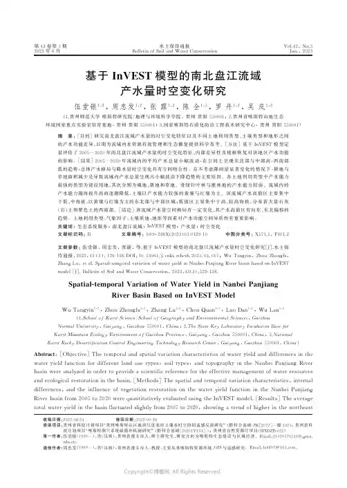
第43卷第3期2023年6月水土保持通报B u l l e t i no f S o i l a n d W a t e rC o n s e r v a t i o nV o l .43,N o .3J u n .,2023收稿日期:2022-08-24 修回日期:2022-09-18资助项目:贵州省科技计划项目 贵州喀斯特山区地块尺度农田土壤水时空协同遥感反演研究 (黔科合基础-Z K [2022]一般302);贵州省科技计划项目 喀斯特洞穴系统碳循环机制研究 (黔科合基础[20201Y 154]);贵州省自然资源厅项目(H X D Z B -022) 第一作者:伍堂银(1999 ),男(汉族),贵州省遵义市人,硕士研究生,研究方向为喀斯特生态建设与区域经济㊂E m a i l :21010170545@g z n u .e d u .c n㊂ 通信作者:周忠发(1969 ),男(汉族),贵州省遵义市人,教授,主要从事喀斯特资源环境㊁G I S 与遥感研究㊂E m a i l :f a 6897@163.c o m ㊂基于I n V E S T 模型的南北盘江流域产水量时空变化研究伍堂银1,2,周忠发1,2,张露1,2,陈全1,3,罗丹1,2,吴岚1,2(1.贵州师范大学喀斯特研究院/地理与环境科学学院,贵州贵阳550001;2.贵州省喀斯特山地生态环境国家重点实验室培育基地,贵州贵阳550001;3.国家喀斯特石漠化防治工程技术研究中心,贵州贵阳550001)摘 要:[目的]研究南北盘江流域产水量的时空变化特征以及不同土地利用类型㊁土壤类型和地形之间的产水功能差异,以期为流域内水资源有效管理和生态修复提供科学参考㊂[方法]基于I n V E S T 模型定量评估了2005 2020年南北盘江流域产水量的时空变化特征㊁内部差异性及植被恢复对该地区产水功能的影响㊂[结果]2005 2020年流域内的平均产水总量小幅波动,在空间上呈现东北部与中部高,西南部低的趋势,总体产水格局与降水量时空变化具有空间吻合性㊂在不考虑降雨量显著变化的情况下,耕地与草地面积减少是导致流域内产水总量呈现出小幅波动下降趋势的主要原因㊂各土地利用类型中产水能力最强的类型为建设用地,其次分别为裸地㊁耕地和草地㊂常绿针叶林与灌林地的产水能力较弱㊂流域内的产水能力随海拔升高而逐渐降低,土壤以产水能力较强的黄壤与红壤为主㊂该流域产水高值区主要集中于低㊁中海拔,以黄壤与红壤为主的东北部与中部区域;低值区主要集中于高㊁较高海拔,分布着大量石灰(岩)土和紫色土的西南部㊂[结论]该流域产水量空间格局有一定变化,其产水高值区有向东㊁东北偏移的趋势㊂土地利用类型㊁气象因子㊁土壤质地㊁地形等因素对产水功能空间异质性有重要影响㊂关键词:生态系统服务;南北盘江流域;I n V E S T 模型;产水量;时空变化文献标识码:B 文章编号:1000-288X (2023)03-0129-10中图分类号:X 171.1,F 301.2文献参数:伍堂银,周忠发,张露,等.基于I n V E S T 模型的南北盘江流域产水量时空变化研究[J ].水土保持通报,2023,43(3):129-138.D O I :10.13961/j .c n k i .s t b c t b .2023.03.017;W u T a n g y i n ,Z h o uZ h o n gf a ,Z h a ng L u ,e t a l .S p a t i a l -t e m p o r a l v a r i a t i o no fw a t e r y i e l d i nN a n b e i P a n j i a n g R i v e r b a s i nb a s e do n I n V E S T m o d e l [J ].B u l l e t i no f S o i l a n d W a t e rC o n s e r v a t i o n ,2023,43(3):129-138.S p a t i a l -t e m p o r a lV a r i a t i o no fW a t e rY i e l d i nN a n b e i P a n j i a n g R i v e rB a s i nB a s e do n I n V E S T M o d e lW uT a n g y i n 1,2,Z h o uZ h o n g f a 1,2,Z h a n g Lu 1,2,C h e nQ u a n 1,3,L u oD a n 1,2,W uL a n 1,2(1.S c h o o l o f K a r s t S c i e n c e /S c h o o l o f G e o g r a p h y an dE n v i r o n m e n t a lS c i e n c e s ,G u i z h o u N o r m a lU n i v e r s i t y ,G u i y a n g ,G u i z h o u 550001,C h i n a ;2.T h eS t a t eK e y L a b o r a t o r y I n c u b a t i o nB a s e fo r K a r s tM o u n t a i nE c o l o g y E n v i r o n m e n t o f G u i z h o uP r o v i n c e ,G u i y a n g ,G u i z h o u 550001,C h i n a ;3.N a t i o n a l K a r s tR o c k y D e s e r t i f i c a t i o nC o n t r o lE n g i n e e r i n g T e c h n o l o g y R e s e a r c hC e n t e r ,G u i y a n g ,G u i z h o u 550001,C h i n a )A b s t r a c t :[O b j e c t i v e ]T h e t e m p o r a l a n d s pa t i a l v a r i a t i o nc h a r a c t e r i s t i c s o fw a t e r y i e l da n dd i f f e r e n c e s i n t h e w a t e r y i e l d f u n c t i o nf o rd i f f e r e n t l a n du s e t y p e s ,s o i l t y p e s ,a n dt o p o g r a p h y i nt h eN a nb e iP a n j i a n g Ri v e r b a s i nw e r e a n a l y z e d i no r d e r t o p r o v i d e a s c i e n t i f i c r e f e r e n c e f o r t h e e f f e c t i v em a n a ge m e n t o fw a t e r r e s o u r c e s a n d e c o l o g i c a l r e s t o r a t i o n i n t h e b a s i n .[M e t h o d s ]T h e s p a t i a l a n d t e m p o r a l v a r i a t i o n c h a r a c t e r i s t i c s ,i n t e r n a l d if f e r e n c e s ,a n d t h e i n f l u e n c eo fv eg e t a t i o nr e s t o r a t i o no nth ew a t e r yi e l df u n c t i o ni nt h eN a n b e iP a nj i a n gR i v e rb a s i n f r o m2005t o 2020w e r e q u a n t i t a t i v e l y e v a l u a t e d u s i n g t h e I n V E S T m o d e l .[R e s u l t s ]T h e a v e r a ge t o t a lw a t e r y i e l d i n t h eb a s i nf l u c t u a t e d s l igh t l y f r o m2005t o 2020,s h o wi n g a t r e n do f h i gh e r i n t h en o r t h e a s t Copyright ©博看网. All Rights Reserved.a n d c e n t r a l r e g i o n s a n d l o w e r i n t h e s o u t h w e s t.T h e o v e r a l lw a t e r y i e l d p a t t e r nw a s s p a t i a l l y c o n s i s t e n tw i t h t h e s p a t i a l a n d t e m p o r a l c h a n g e s o f p r e c i p i t a t i o n.W i t h o u t c o n s i d e r i n g t h e s i g n i f i c a n t c h a n g eo f r a i n f a l l,t h e d e c r e a s e o f c u l t i v a t e d l a n d a n d g r a s s l a n d a r e a sw a s t h em a i n r e a s o n f o r t h e s l i g h t f l u c t u a t i o na n dd o w n w a r d t r e n do f t o t a l w a t e r y i e l d i n t h eb a s i n.T h e l a n d u s e t y p ew i t h t h e s t r o n g e s tw a t e r y i e l dc a p a c i t y w a s c o n s t r u c t i o n l a n d,f o l l o w ed b y b a r el a n d,c u l t i v a te dl a n d,a n d g r a s s l a n d.T h e w a t e r y i e l d c a p a c i t i e s o fe v e r g r e e n c o n if e r o u s f o r e s t a n d s h r u b l a n dw e r ew e a k.T h ew a t e r y i e l dc a p a c i t y i nt h eb a s i ng r a d u a l l y d e c r e a s e dw i thi n c r e a s i n g a l t i t u d e,a n d t h e s o i l sw i t hs t r o n g w a t e r y i e l dc a p a c i t y w e r em a i n l yy e l l o ws o i l a n dr e ds o i l.T h e h i g hw a t e r y i e l d a r e a s i n t h eb a s i nw e r em a i n l y c o n c e n t r a t e d i n t h en o r t h e a s t a n d c e n t r a l r e g i o n sh a v i n g l o w a n dm e d i u ma l t i t u d e s,a n dw e r em a i n l yy e l l o ws o i l a n d r e d s o i l.T h e l o wv a l u e a r e aw a sm a i n l y c o n c e n t r a t e d i n t h e s o u t h w e s t r e g i o nh a v i n g h i g ha n dh i g h e r a l t i t u d e sw i t h l a r g e a m o u n t so f l i m e(r o c k)s o i l a n d p u r p l e s o i l.[C o n c l u s i o n]T h e s p a t i a l p a t t e r no fw a t e r y i e l d i n t h e b a s i n e x h i b i t e d s o m e c h a n g e s,a n d t h e h i g hv a l u e a r e a o fw a t e r y i e l dh a d a t e n d e n c y t o s h i f t t o t h e e a s t a n dn o r t h e a s t.L a n du s e t y p e,m e t e o r o l o g i c a l f a c t o r s, s o i l t e x t u r e,t o p o g r a p h y,a n do t h e rf a c t o r sh a v ea ni m p o r t a n t i m p a c to nt h es p a t i a lh e t e r o g e n e i t y o f t h e w a t e r y i e l d f u n c t i o n.K e y w o r d s:e c o s y s t e ms e r v i c e s;N a n b e i P a n j i a n g R i v e r b a s i n;I n V E S Tm o d e l;w a t e r y i e l d;t e m p o r a l a n d s p a t i a l v a r i a t i o n c h a r a c t e r i s t i c s生态系统服务是指人类从生态系统中直接或间接获得(包括有形产品以及无形服务在内)的所有惠益[1],而生态系统服务评估则是对生态系统所提供和维持的进行定量表达[2]㊂2005年联合国发布的千年生态系统评估报告中指出,全球60%的生态系统服务发生了退化[3]㊂水作为生命之源,是生物生存不可或缺的部分,在生态系统内转换㊁运移等过程中能够产生多种服务效应[4]㊂因此,如何实现生态系统产水服务功能的空间可视化与定量化评估已成为区域可持续发展的关键[5]㊂随着高空间分辨率数据集和各种水文模型的应用,国内外学者基于不同样本区㊁景观类[6]㊁区域和全球尺度[7],对流域[8]㊁河流[9]㊁湿地[10]等不同研究对象进行生态系统服务功能的评估研究,如M I K E S H E 模型㊁S WA T模型㊁T O P MO D E L模型和I n V E S T模型等[11]㊂其中,I n V E S T模型以水量平衡法为基础,与传统的土壤蓄水能力法[12]㊁综合蓄水能力法[13]㊁多因子分析法[14]等方法相比,考虑了区域蒸散发量的影响,具有结构简单㊁输入参数获取便捷㊁全球通用㊁能够可视化产水功能的空间特征等优点㊂在一定程度上解决了评估结果实用性差㊁服务功能形成机制不明确等问题,为评估产水服务功能提供了新的视角[15]㊂近年来,有关I n V E S T模型在国内外的应用已较为成熟,国外学者基于I n V E S T模型评估了非洲科特迪瓦[16]㊁西班牙F r a n c o l i流域[17]㊁尼泊尔B a g m a t i流域[18]等地的水源涵养进行评估,且模拟结果及运用较好;国内学者基于I n V E S T模型对喀斯特山区[19]㊁黄土高原地区[20]㊁黑河流域[21]㊁三江源地区[22]㊁横断山区[23]等的产水量或水源涵养及其时空变化特征进行了评价,模拟结果均得到了较好的应用效果㊂南北盘江流域作为珠江流域的上游,是珠江流域极为重要的水源地㊂流域内石灰岩广泛发育且土层浅薄㊁生态承载力较低㊁石漠化发育剧烈,是珠江流域水土流失最严重的地区[24]㊂目前,已有学者对南北盘江流域的森林生态系统水源涵养[13]㊁生态修复与水土保持[25-26]㊁水质净化[27]㊁地下水资源评价[28]㊁生境质量评价[29]㊁土地利用变化与气候变化对径流影响[30-31]等进行研究,但多数学者仅对单一的土地利用类型进行研究,忽略了其他土地利用类型以及土壤㊁地形因素对流域产水量的影响㊂因此,以南北盘江流域为整体的评价单元,对所有土地利用类型㊁不同土壤类型以及不同地形产水量进行量化评价的研究还需要深入研究㊂本研究运用I n V E S T模型中的产水量模块,结合 3S 技术,克服了传统方法在研究尺度和跨省研究的局限性,从时间和空间两个角度上对南北盘江流域的产水服务功能进行评估,探究多年间南北盘江流域产水功能的时空变化特征㊁内部差异性及植被恢复对该地区产水功能的影响,以期为南北盘江流域退耕还林还草工程㊁水资源管理提供科学参考㊂1研究区概况南北盘江流域(图1)(102ʎ15' 106ʎ22'E, 23ʎ8' 26ʎ54'N)作为珠江流域的上游,发源于云南省沾益县马雄山,是珠江流域极为重要的水源地,干流全长分别为914.5k m和449k m,流经云南㊁贵州㊁031水土保持通报第43卷Copyright©博看网. All Rights Reserved.广西3个省份,流域面积约81764.2k m2[32]㊂境内地势西北高东南低,地貌发育强烈且类型繁多,属于亚热带季风气候,主要植被类型为常绿㊁落叶阔叶林和针叶林,5 10月为雨季,11 次年4月为旱季,降雨大部分集中在雨季,年平均气温12.65~21.25ħ,年平均降水量930.38~1281.12mm[13]㊂南北盘江流域内70%地区属于碳酸盐岩地层,且盘江中上游含煤岩组广泛发育,其余地区属于二叠系玄武岩及侏罗系砂岩,石灰岩分布广泛,属于中国典型的喀斯特生态脆弱区,主要土壤类型为红壤㊁黄壤㊁石灰土㊁紫色土等㊂注:本图基于[黔S(2023)009号㊁云S(2020)102号㊁桂S(2020) 48号]标准地图校稿制图㊂下同㊂图1南北盘江流域研究区概况F i g.1O v e r v i e wo f s t u d y a r e a i nN a n b e i P a n j i a n g R i v e r b a s i n 2数据来源与研究方法2.1数据来源本研究涉及的产水量模块输入数据主要包括30m D E M数据㊁土地利用㊁气象数据㊁土壤数据㊁植被可利用水㊁生物物理参数表㊁流域边界等数据㊂研究所有影像数据空间分辨率均重采样到30m,坐标系均使用中国大地坐标系(C G C S2000)㊂土地利用数据(空间分辨率为30m)下载于中国科学院空天信息创新研究院(h t t p:ʊw w w.a i r c a s.c a s.c n/);气象数据来源于国家气象科学数据中心(h t t p:ʊd a t a.c m a.c n/);土壤数据来源于国家科技资源共享服务平台 国家地球系统科学数据中心 土壤分中心(h t t p:ʊs o i l.ge o d a t a.c n/);30m D E M数据来源于地理空间数据云(h t t p:ʊw w w.g s c l o u d.c n/);流域边界在国家地球系统科学数据中心(2000年)公布的南北盘江流域边界的基础上,利用A r c G I S水文分析工具进行提取;生物物理参数(表1)来源于文献查阅[20-33]以及‘I n V E S T使用指南“㊂表1产水量模型中不同土地利用类型的参数T a b l e1P a r a m e t e r s o f d i f f e r e n t l a n du s e t y p e s i nw a t e r y i e l dm o d e l地类L u c o d e r o o t_d e p t h K c L U L C_v e g 耕地120000.651常绿阔叶林2500011落叶阔叶林3500011常绿针叶林4500011灌林地530000.91草地626000.651湿地710000.650建设用地810.10裸地910.51水域10100永久冰雪11100注:L u c o d e为地类编号;K c为每一地类对应的植被蒸散系数; r o o t_d e p t h为每一地类植物的最大根系深度(mm);L U L C_v e g的赋值是既定规则;植被覆盖地类(不包括湿地)赋值为1;其他土地利用类型(包括湿地㊁城市用地㊁水体㊁永久冰雪)赋值为0㊂2.2研究方法本研究运用I n V E S T模型中的产水量模块模拟南北盘江流域产水量空间分布格局㊂产水量模块是根据水量平衡为基本原则的一种估算方法,在栅格尺度上通过降水量减去实际蒸散量(包含地面蒸发量与植被蒸腾量)得到栅格水平的产水量,该模块不能区分地表水㊁地下水㊁基流,而是假设每个栅格级别的产水通过地下径流或地表径流的方式到达流域出水口[34]㊂主要算法如下:Y x j=1-A E T x jP xˑP x(1)式中:Y x j是栅格x单位上的第j种土地覆盖类型的年产水量(mm);A E T x j是栅格x单位上的第j种土地覆盖类型的年实际蒸散量(mm);P x为栅格x上的年平均降水量(mm)㊂其中,根据Z h a n g等基于B u d y k o提出的水-热耦合平衡假定计算出的蒸散部分A E T x jP x(实际蒸散量与降水量比值),其表达公式如下:A E T x jP x=1+ωx R x j1+ωx R x j+1/R x j(2)式中:R x j为第j土地利用类型栅格x的B u d y k o干燥指数;ωx表示植被有效含水量与年均降水量的比值:131第3期伍堂银等:基于I n V E S T模型的南北盘江流域产水量时空变化研究Copyright©博看网. All Rights Reserved.ωx=Z AW C x P x(3)R x j=K x j E T0xP x(4) AW C x=M i n(D s,D r)ˑP AW C x(5)式中:AW C x为栅格x的植被有效含水量(mm)(由有效土层深度和土壤质地决定);Z为季节参数(即Z h a n g系数)用于表征降水的季节性特征;K x j为第j 土地利用类型栅格x的植被蒸散系数;E T0x表示栅格x的潜在蒸散量(mm);D s为土层深度(mm);D r为根系深度(mm);P AW C x为栅格单元x的植物可利用水含量(mm),植物可利用含水量P AW C 可以通过土壤质地以及土壤有机质含量计算得到,其表达公式如下:P AW C=54.509-0.132ˑs a n d%-0.003(s a n d%)2-0.055ˑs i l t%-0.006(s i l t%)2-0.738ˑc l a y%+ 0.007(c l a y%)2-2.688ˑOM%+ 0.501(OM%)2(6)式中:s a n d%,s i l t%,c l a y%分别表示土壤砂粒㊁粉粒㊁黏粒的比例;OM%则表示土壤有机质含量㊂3结果与分析3.1南北盘江流域产水量的时空变化特征应用I n V E S T模型产水模块对南北盘江流域2005 2020年产水量进行评估,以2005年为基准年,Z参数以年为尺度,不考虑季节变化㊂根据贵州㊁云南㊁广西三省的水资源公报流域实测站点数据,经模拟计算,发现当Z值为30时,I n V E S T产水模块模拟值效果最佳㊂根据模拟结果,南北盘江流域2005 2020年平均降雨量和平均产水总量分别为1162.1,677.2ˑ108m3,平均产水深度为828.0mm㊂从空间分布格局来看(图2),南北盘江流域产水量在2005 2020年空间分布格局与降雨量均相似,这与南北盘江流域降水分布东北多西南少㊁实际蒸散量分布东北少西南多,以及土地覆盖类型变化差异有着密切的关系,主要呈现为东北部和中部高㊁西南部低的趋势㊂产水量高值区主要集中于流域中部及东北部,即贵州省境内的安龙县㊁贞丰县㊁兴仁县㊁盘州市和云南省境内的富源县㊁罗平县一带;而区域产水量低值区主要集中于流域西南部,即云南省境内的通海㊁丘北㊁华宁县以及江川县一带㊂图22005—2020年南北盘江流域产水量及降雨量分布F i g.2W a t e r y i e l da n d r a i n f a l l d i s t r i b u t i o n i nN a n b e i P a n j i a n g R i v e r b a s i n f r o m2005t o2020从时间尺度来看(图3),2005 2020年,南北盘江流域平均总产水量变化趋势表现为先减小后增大,再减小的波动变化㊂2005 2010年,产水深度小幅度减小,减小幅度为10.1%;2010 2015年,产水深度明显增加,增加幅度约为19.3%;2015 2020年,产水深度大幅度减小,减少量为177.8mm(19.3%)㊂总体来看,产水量呈现出在828.3mm上下幅度20.0%之间波动趋势,2005年和2015年产水量处于高水平状态,2010年和2020年产水量处于低水平状态㊂231水土保持通报第43卷Copyright©博看网. All Rights Reserved.图32005 2020年南北盘江流域产水深度㊁降雨量㊁产水总量以及实际蒸发量F i g.3W a t e r y i e l dd e p t h,r a i n f a l l,t o t a l w a t e r y i e l da n da c t u a l e v a p o r a t i o n i nN a nb e i P a n j i a n g R i v e r b a s i nf r o m2005t o20202005 2010年(图4a),流域内年平均产水深度显著减小面积约占研究区总面积的46.9%,产水量减小区域主要集中在研究区中部和南部边缘地带;增加区域较小,约占研究区面积的2.8%,主要集中在西部边缘地带㊂2010 2015年(图4b),在产水量显著增加期间,其产水量增加面积约占研究区总面积的69.9%,增加区域分布于整个研究区,产水量减少区域仅分布于研究区北角处(3.8%)㊂2015 2020年(图4c),以极显著减小与显著减小为主面积约占研究区总面积的70.7%,其空间格局与2010 2015年相反,减小区域分布于整个研究区㊂总体而言,2005 2020年(图4d),产水量极显著减小区域约占整个研究区的11.7%,主要集中在研究区中部,约9.8%的产水量显著增加区域分布于研究区的北部㊂结果表明, 2005 2020年南北盘江流域产水能力在空间分布上呈现出由西南向东北递增㊂图42005 2020年南北盘江流域产水量年际变化F i g.4I n t e r a n n u a l v a r i a t i o no fw a t e r y i e l d i nN a n b e i P a n j i a n g R i v e r b a s i n f r o m2005t o20203.2不同土地利用类型下的产水功能差异产水总量在受产水面积和单位面积产水能力的双重约束之下,在不同的土地利用类型上也存在区别㊂以2020年为例(表2),南北盘江流域的主要土地利用类型为林地㊁耕地和草地,三者都具有较高的产水能力,分别占研究区总面积的52.6%,24.8%和14.5%㊂通过产水贡献率(即不同土地利用类型的产水总量与流域的总产水总量的比值)来衡量不同土地331第3期伍堂银等:基于I n V E S T模型的南北盘江流域产水量时空变化研究Copyright©博看网. All Rights Reserved.利用类型的产水总量贡献㊂因此,林地㊁耕地和草地是南北盘江流域产水总量的主要贡献者,为整个南北盘江流域提供了96.4%的产水总量,建设用地提供了研究区3.0%的产水总量,湿地㊁水域㊁裸地以及永久冰雪的产水总量比例共为0.6%(图5)㊂根据I n V E S T 模型‘用户指南“,模型自身将湿地㊁建设用地㊁水域㊁永久冰雪赋值为非植被覆盖地类(表1),故除建设用地之外的非植被覆盖地类不在本研究讨论范围内㊂表22005 2020年南北盘江流域各土地利用类型转移矩阵变化率T a b l e2C h a n g e r a t e o f t r a n s f e rm a t r i x o f l a n du s e t y p e s i nN a n b e i P a n j i a n g R i v e r b a s i n f r o m2005t o2020项目2005年面积变化率/%耕地常绿阔叶林落叶阔叶林常绿针叶林灌林地草地湿地建设用地裸地水域永久冰雪合计% /率化变积面年0 2 0 2耕地24.140.320.320.200.260.200.000.680.000.040.0026.16常绿阔叶林0.059.750.080.110.070.01 0.010.00 10.07落叶阔叶林0.070.1115.510.090.050.04 0.010.00 15.88常绿针叶林0.250.100.1225.570.040.21 0.050.000.020.0026.34灌林地0.020.100.030.013.910.010.00 0.00 4.08草地0.310.010.070.170.0114.070.000.190.000.010.0014.84湿地 0.00 0.00建设用地 1.69 1.69裸地 0.00 0.00水域0.010.000.000.000.000.000.000.000.000.92 0.94永久冰雪 0.000.00合计24.8610.3816.1226.154.3314.520.002.630.001.000.00100注: 表示该土地利用类型没有发生变化; 0.00 代表该土地利用类型发生变化且转换率较小;粗体数值为未发生变化的土地利用类型的保留率㊂图52005 2020年南北盘江流域各土地利用类型年产水深度及产水总量变化F i g.5C h a n g e s o f a n n u a l w a t e r y i e l dd e p t ha n d t o t a l w a t e ry i e l do f d i f f e r e n t l a n du s e t y p e s i nN a n b e i P a n j i a n gR i v e r b a s i n f r o m2005t o2020由图5可知,在时间变化上,除耕地㊁草地㊁裸地和建设用地外,其余土地利用类型的年产水深度与研究区整体变化相似,即表现为先减小后增大,再减小的波动变化㊂总体看来,以2020为例,产水能力强弱表现为:建设用地(1033mm)>裸地(887mm)>耕地(851)>草地(810mm)>落叶阔叶林(738mm)>常绿阔叶林(682mm)>常绿针叶林(637mm)>灌木林(608mm)㊂其中,根据产水模块机理,产水量与蒸散量成反比关系,建设用地面积约占研究区面积2.6%,主要以不透水面为主,植被覆盖度低,导致其蒸散量小,因此具有较高的产水能力;耕地的表层土壤由于长期受人类活动影响呈现出退化㊁板结㊁孔隙度降低,导致其产水能力略高㊂自 十五 计划实施以来,正式全面启动退耕还林(草)生态工程,研究区耕地面积持续减少,林地面积持续增加,但草地面积持续减少㊂林草覆盖率由2005年的71.2%上升至2020年的71.5%,约增加了244.31k m2,但由于草地面积减少了259.22k m2,约为林地增加面积的二分之一,且草地产水能力优于林地,导致林草部分的产水总量减少了7.62ˑ109m3;同时,耕地面积持续减少,产水总量减少了2.45ˑ109m3㊂因此,耕地与草地面积减少是导致流域内产水总量呈现出小幅波动下降趋势的主要原因之一㊂由表3可知,2005 2020年,研究区内耕地㊁草地以及常绿阔叶林面积均呈现出不同程度的下降趋势㊂其中耕地面积持续减少最严重,约为1063.4k m2,减小幅度为5.0%;草地㊁常绿针叶林面积分别缩减了259.2m2,157.9k m2,减幅分别达到了2.1%和0.7%㊂建设用地面积持续增加,约为770.5k m2,增加幅度为了55.7%;常绿阔叶林㊁灌林地㊁落叶阔叶林以及裸地面积增幅分别为3.1%,6.2%,1.5%和44.8%㊂表明南北盘江流域在城市化的进程中,大量的耕地转变431水土保持通报第43卷Copyright©博看网. All Rights Reserved.为建设用地,加上退耕还林(草)生态工程的实施,还有一部分耕地转换为常绿阔叶林㊁落叶阔叶林㊁常绿针叶林㊁草地以及灌林地,导致耕地面积持续减少㊂受人类耕作影响下,草地主要转换为耕地和建设用地,常绿针叶林主要转换为耕地,且草地与常绿针叶林受人类耕作影响转出面积,大于受生态修复工程影响转入面积,导致草地与常绿针叶林面积均呈现出小幅度下降趋势㊂表32005 2020年南北盘江流域各土地利用类型面积变化及变化率T a b l e3A r e a c h a n g e a n d c h a n g e r a t e o f e a c h l a n du s e t y p e i nN a n b e i P a n j i a n g R i v e r b a s i n f r o m2005t o2020土地利用类型2005 2010年面积变化/k m2变化率/%2010 2015年面积变化/k m2变化率/%2015 2020年面积变化/k m2变化率/%2005 2020年面积变化/k m2变化率/%耕地-351.64-1.64-417.19-1.98-294.57-1.43-1063.40-4.97常绿阔叶林71.780.8794.381.1488.731.06254.903.10落叶阔叶林42.670.3373.640.5783.280.64199.591.54常绿针叶林17.920.08-83.03-0.39-92.82-0.43-157.93-0.73灌林地55.851.6764.211.8986.902.51206.976.20草地-108.27-0.89-53.45-0.44-97.50-0.81-259.22-2.14湿地0.072.490.299.990.185.660.5519.12建设用地253.5918.33311.9119.05204.9610.52770.4655.69裸地0.047.080.0611.160.1421.660.2444.81水域17.962.349.141.1620.642.6047.746.23永久冰雪0.0214.580.0211.360.0315.100.0846.873.3不同海拔下的产水量功能差异研究区海拔分布规律呈现自西北向东南递减的趋势,与产水量能力空间分布特征呈现出明显的差异性㊂云贵高原属于中国地形的第二阶梯,海拔主要在1~2k m之间,将研究区高程(图6a)分为低㊁中㊁高㊁较高海拔4个级别,海拔等级呈正态分布,即海拔小于900m的面积占比为8.33%,900~1400m (24.02%),1400~1900m(39.19%),海拔大于1900m的面积比例为28.45%,其产水总量贡献率分别为9.83%,26.68%,37.97%和25.52%㊂在海拔1400~1900m之间的面积比例与产水总量贡献率最大,海拔小于900m的面积比例与产水总量贡献率最小;就平均产水深度而言(图7),随着海拔等级升高而逐渐降低,低㊁中海拔区域具有较强的产水能力,高㊁较高海拔区域的产水能力相对较弱㊂其中,海拔小于900m的产水深度最大,约为1068.57mm ㊂图6南北盘江流域D E M数据㊁土壤类型以及土层厚度F i g.6D E Md a t a,s o i l t y p e a n d s o i l t h i c k n e s s i nN a n b e i P a n j i a n g R i v e r b a s i n3.4不同土壤类型下的产水量功能差异如图8所示,在土壤类型上,产水能力的大小依次为:黄棕壤>水稻土>红壤>黄壤>紫色土>石灰(岩)土㊂红壤与黄壤是流域内地带性土壤,集中连片分布于流域中部和西部,占研究区总面积比例较大,分别为40.44%和32.72%;其次主要为水稻土(9.76%)㊁石灰(岩)土(9.42%)㊁紫色土(3.49%)以及黄棕壤(2.45%)等㊂本文仅考虑面积比例较大的土壤类型,其产水总量贡献率分别为红壤(43.12%)㊁黄壤(33.70%)㊁水稻土(9.33%)㊁石灰(岩)土(7.95%)㊁531第3期伍堂银等:基于I n V E S T模型的南北盘江流域产水量时空变化研究Copyright©博看网. All Rights Reserved.紫色土(3.08%)和黄棕壤(2.81%)㊂红壤和黄壤所含有机质㊁铁铝含量高,土壤肥力条件较好,耐旱保肥,适宜植被生长;石灰(岩)土和紫色土属于初育土,植被大多较为稀疏㊂大部分土壤的涵蓄降水量能力随土层厚度加深而增加,根据‘国家森林资源连续清查主要技术规定(2003年10月修订版)“,将研究区土层厚度(图6c)划分为薄(0 80c m)㊁中(80 100c m)和厚(ȡ100c m)3个厚度级别,研究区土层厚度主要以中级厚度为主,包含了研究区内大部分红壤与黄壤,使得流域内土壤的涵蓄降水量能力保持在一定水平上㊂图7南北盘江流域不同海拔的面积比例㊁产水差异和产水总量F i g.7A r e a p r o p o r t i o n,w a t e r y i e l dd i f f e r e n c e a n d t o t a l w a t e ry i e l da t d i f f e r e n t a l t i t u d e s i nN a n b e i P a n j i a n g R i v e r b a s i n图8南北盘江流域不同土壤类型的面积比例㊁产水差异和产水总量F i g.8A r e a p r o p o r t i o n,w a t e r y i e l d d i f f e r e n c e a n d t o t a l w a t e r y i e l d o fd i f fe r e n t s o i l t y p e s i nN a n b e i P a n j i a n g R i v e r b a s i n3.5各要素对产水功能的综合影响由图9可知,流域内植被在海拔上呈现出明显的垂直地带性㊂常绿阔叶林与灌林地的面积占比随海拔等级升高而降低;常绿针叶林与草地相反,其面积占比在海拔等级上呈 倒金字塔 状分布;常绿阔叶林的面积占比呈 衰退型 分布;耕地面积占比在各级海拔均约为四分之一,属于 稳定型 分布㊂由图10可知,除低海拔(<900m)外,红壤与水稻土面积占比随海拔等级升高而降低,黄壤面积占比随海拔等级升高而增加;初育土(包含石灰土和紫色土)面积占比随海拔等级升高而增加㊂在低㊁中海拔区域内,产水能力较强的耕地㊁落叶阔叶林与常绿阔叶林面积占比较大,常绿针叶林占比较小,且产水能力较差的初育土面积占比最小,红壤面积占比较大,是导致低㊁中海拔区产水能力偏高的主要原因之一;在高㊁较高海拔区域内,产水能力较弱的常绿针叶林面积占比最大,落叶阔叶林与常绿阔叶林面积占比较小,且初育土面积占比增大,红壤面积占比减小,是导致高㊁较高海拔区产水能力偏低的主要原因之一㊂虽然建设用地和裸地的产水能力较强,但其总面积较小,对区域的整体产水能力影响可忽略不计㊂图9南北盘江流域不同海拔等级下的土地利用类型比例F i g.9P r o p o r t i o no f l a n du s e t y p e s a t d i f f e r e n t a l t i t u d e s i nN a n b e i P a n j i a n g R i v e r b a s i n图10南北盘江流域不同海拔等级下的土壤类型比例F i g.10P r o p o r t i o no f s o i l t y p e s a t d i f f e r e n t a l t i t u d e s i nN a n b e i P a n j i a n g R i v e r b a s i n综合各方面因素,流域东北部和中部区域在空间上属于降雨量的高值区,位于低㊁中海拔区域,落叶阔叶林与常绿阔叶林面积占比较大,常绿针叶林占比较631水土保持通报第43卷Copyright©博看网. All Rights Reserved.小,且土壤类型主要以产水能力较强的黄壤和红壤为主㊂流域西南部区域是降雨量的低值区,位于高海拔区域,常绿针叶林面积比例较大,落叶阔叶林与常绿阔叶林面积比例较小,且分布着大量产水能力较弱的石灰(岩)土和紫色土,使得2005 2020年南北盘江流域产水格局均呈现出东北部和中部高㊁西南部低的趋势㊂4讨论与结论4.1讨论南北盘江流域产水量年际间的波动与气候变化有密切关系,而降水量在时空分异特征上与产水量呈显著正相关关系㊂研究显示流域产水量存在峰值和低谷㊂臧文斌等[35]和贺敏等[36]基于数据表明西南地区2015年降雨量充沛,2020年降雨量较少,与该流域产水量年际间的波动变化相吻合㊂流域由于地形西高东低,夏季携带大量水汽的气流受地形抬升作用下,在流域东北部凝结降落,使该流域降雨量空间分布格局呈现出自东北向西南递减,与莫旭昱等[37]对南北盘江流域降水的空间格局分析结果相一致㊂流域产水能力随着海拔升高而逐降低,这与谢余初等[11]在白龙江流域研究结果相似,与王晓峰等[38]在秦岭地区研究的结果相反,是因为白龙江流域是秦岭的子流域之一,因研究尺度不同所导致的规律差异㊂一方面,二者面积上差距大;另一方面,对应的海拔产水功能含义有所区别,前者将流域视为整体,再对海拔进行划分,而后者将流域视为整体的同时,再进行子流域划分,以子流域为研究单元研究㊂本研究以年为尺度对该流域产水量进行模拟,模拟结果基本符合区域的实际情况,但侧重于分析自然因子对产水服务的影响,忽略了社会因子的影响㊂同时,因模型自身设定及数据精度㊁未考虑流域产水的年内变化等原因,在一定程度上会影响模型的模拟精度㊂但产水量的基本格局不会改变,该研究成果仍然能较好地反映出南北盘江流域产水量的时空变化特征及趋势,从而为南北盘江流域水资源的有效管理㊁合理利用与保护提供了科学依据㊂后续的研究中可从小尺度着手,在明晰流域总体产水量时空格局的基础上进一步挖掘异常或者特殊区域产水服务的特殊时空变化规律㊂同时,产水量仅是流域内生态系统服务中的一项指标,应综合考虑各项服务效益,科学地去权衡各服务之间的关系㊂4.2结论(1)从空间分布格局来看,南北盘江流域产水强度高值区有向东㊁东北偏移的趋势㊂总体产水格局维持与降水量的空间吻合性,呈现出东北部和中部高㊁西南部低的趋势㊂产水量高值区主要位于贵州省境内的安龙县㊁贞丰县㊁兴仁县和盘州特区和云南省境内的富源县㊁罗平县一带,产水量低值区则主要集中于云南省境内的通海县㊁丘北县㊁华宁县和江川县一带㊂2005 2020年,该流域的平均产水总量与降水量在时间上具有一致性,整体呈现出先减小后增大,再减小的小幅波动下降趋势㊂(2)在土地利用类型方面,林地㊁耕地和草地是南北盘江流域产水总量的主要贡献者,提供了整个南北盘江流域总产水量的92.8%;产水能力大小依次为:建设用地>裸地>耕地>草地>落叶阔叶林>常绿阔叶林>常绿针叶林>灌木林㊂期间,建设用地与林地面积持续增加,耕地和草地面积持续减小;在城市化进程与人类活动影响下,主要的土地转变方式:耕地主要转变为建设用地㊁林地和草地;草地主要转变为耕地和建设用地;林地主要转变为耕地和草地㊂(3)在垂直梯度上,流域产水能力随着海拔升高而逐降低㊂在土壤类型上,产水能力的大小依次为:黄棕壤>水稻土>红壤>黄壤>紫色土>石灰(岩)土,红壤和黄壤是流域内面积最大的地带性土壤,是流域内产水总量稳定的重要保障㊂自 十五 期间全面启动退耕还林(草)生态工程以来,研究区耕地㊁草地面积持续减少㊂在不考虑降雨量显著变化的情况下,耕地与草地面积减少是导致流域内产水总量呈现出小幅波动下降趋势的主要原因㊂[参考文献][1] S o n g F e n g j i a o,W a n g S h i j i e,B a i X i a o y o n g,e t a l.An e wi n d i c a t o r f o r g l o b a l f o o d s e c u r i t y a s s e s s m e n t:H a r v e s t e da r e a r a t h e r t h a n c r o p l a n d a r e a[J].C h i n e s eG e o g r a p h i c a lS c i e n c e,2022,32(2):204-217.[2] T u r n e rR K,D a i l y GC.T h e e c o s y s t e ms e r v i c e s f r a m e-w o r ka n dn a t u r a l c a p i t a l c o n s e r v a t i o n[J].E n v i r o n m e n t a la n dR e s o u r c eE c o n o m i c s,2008,39(1):25-35.[3] F i n l a y s o n M,C r u zRD,D a v i d s o nN,e t a l.M i l l e n n i u me c o s y s t e m a s s e s s m e n t:e c o s y s t e m s a n d h u m a n w e l l-b e i n g:w e t l a n d sa n d w a t e rs y n t h e s i s[J].D a t aF u s i o nC o n c e p t s&I d e a s,2005,656(1):87-98.[4]吕一河,胡健,孙飞翔,等.水源涵养与水文调节:和而不同的陆地生态系统水文服务[J].生态学报,2015,35(15):5191-5196.[5] B e n n e t tE M,P e t e r s o nG D,G o r d o nLJ.U n d e r s t a n d i n gr e l a t i o n s h i p sa m o n g m u l t i p l ee c o s y s t e m s e r v i c e s[J].E c o l o g y L e t t e r s,2009,12(12):1394-1404.[6]张彪,李文华,谢高地,等.北京市森林生态系统的水源涵养功能[J].生态学报,2008,28(11):5619-5624.731第3期伍堂银等:基于I n V E S T模型的南北盘江流域产水量时空变化研究Copyright©博看网. All Rights Reserved.。

第44卷 第4期Vol.44, No.4, 323~3362015年7月GEOCHIMICAJuly, 2015收稿日期(Received): 2014-08-18;; 改回日期(Revised): 2014-11-10; 接受日期(Accepted): 2014-12-19基金项目: 国家自然科学基金(41473122, 41073096); 国家重点基础研究发展计划项目(2013CB956702); 中国科学院“百人计划”项目作者简介: 张莉(1989–), 女, 硕士研究生, 主要研究方向为环境地球化学。

E-mail: gzsdzl@ * 通讯作者(Corresponding author): JI Hong-bing, E-mail: jih_0000@, Tel: +86-10-68909710ZHANG Li et al .: Geochemistry of elements in typical carbonate weathered profiles of Guizhou Plateau贵州碳酸盐岩风化壳主元素、微量元素及稀土元素的地球化学特征张 莉1, 季宏兵1,2*, 高 杰1, 李 锐1, 李今今1(1. 首都师范大学 资源环境与旅游学院 首都圈生态环境过程重点实验室, 北京 100048; 2. 中国科学院 地球化学研究所 环境地球化学国家重点实验室, 贵州 贵阳 550002)摘 要: 选取贵州高原喀斯特地区的典型碳酸盐岩原生风化剖面为研究对象, 研究主元素、微量元素及稀土元素在风化壳的迁移转化及其分布规律特征, 为解释碳酸盐岩风化壳元素的地球化学变化提供依据。

结果显示, 从上陆壳标准化蛛网图可知, Pb 、Co 在剖面富集, 而Na 、K 、Cr 、Rb 、Sr 和Ba 则亏损。

风化壳∑REE 的变化范围为167.4~1814.2 μg/g, 稀土元素从剖面下部往上逐渐减少, 剖面中上部LREE 比HREE 淋滤程度大。

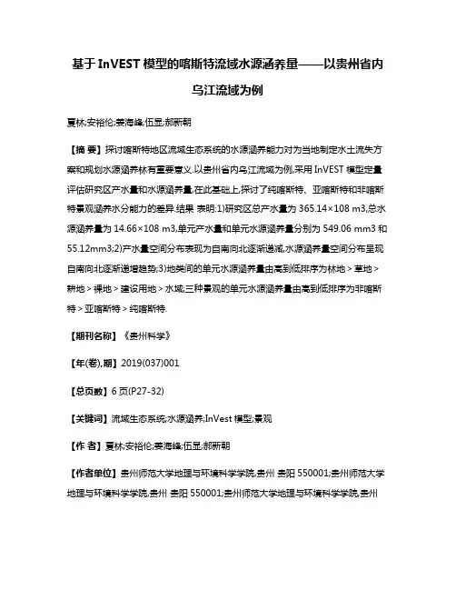
基于InVEST模型的喀斯特流域水源涵养量——以贵州省内乌江流域为例夏林;安裕伦;姜海峰;伍显;郝新朝【摘要】探讨喀斯特地区流域生态系统的水源涵养能力对为当地制定水土流失方案和规划水源涵养林有重要意义.以贵州省内乌江流域为例,采用InVEST模型定量评估研究区产水量和水源涵养量,在此基础上,探讨了纯喀斯特、亚喀斯特和非喀斯特景观涵养水分能力的差异.结果表明:1)研究区总产水量为365.14×108 m3,总水源涵养量为14.66×108 m3,单元产水量和单元水源涵养量分别为549.06 mm3和55.12mm3;2)产水量空间分布表现为自南向北逐渐递减,水源涵养量空间分布呈现自南向北逐渐递增趋势;3)地类间的单元水源涵养量由高到低排序为林地＞草地＞耕地＞裸地＞建设用地＞水域;三种景观的单元水源涵养量由高到低排序为非喀斯特＞亚喀斯特＞纯喀斯特.【期刊名称】《贵州科学》【年(卷),期】2019(037)001【总页数】6页(P27-32)【关键词】流域生态系统;水源涵养;InVest模型;景观【作者】夏林;安裕伦;姜海峰;伍显;郝新朝【作者单位】贵州师范大学地理与环境科学学院,贵州贵阳550001;贵州师范大学地理与环境科学学院,贵州贵阳550001;贵州师范大学地理与环境科学学院,贵州贵阳550001;贵州师范大学地理与环境科学学院,贵州贵阳550001;贵州师范大学地理与环境科学学院,贵州贵阳550001【正文语种】中文【中图分类】P333流域是生态系统中特殊的区域，不仅能调节自然界水循环平衡，而且其水资源在农田灌溉、提供人类生活用水、净化环境、维护生物多样性等方面均有重要贡献[1]。

随着经济快速发展和人口增长，人类无序开发和低效利用使得流域水质持续恶化，水资源短缺受到越来越多人的关注，水源涵养功能已经成为水资源管理所面临的主要挑战[2]。

定量评估流域生态系统水源涵养功能对缓解水资源需求压力、耕地开发与保护等方面均具有重要意义[3]。

第31卷第3期2024年6月水土保持研究R e s e a r c ho f S o i l a n d W a t e rC o n s e r v a t i o nV o l .31,N o .3J u n .,2024收稿日期:2023-07-03 修回日期:2023-07-26 资助项目:国家自然科学基金项目 喀斯特城市景观格局时空演变及其对山体植物多样性影响的尺度效应 (42061039);贵州大学培育项目 喀斯特山地城市生物多样性维持的景观恢复力机制研究 (贵大培育[2020]46) 第一作者:李井浩(2001 ),男,重庆开州人,硕士研究生,主要从事景观与区域生态研究㊂E -m a i l :3354546236@q q.c o m 通信作者:王志杰(1986 ),男,甘肃会宁人,博士,教授,主要从事景观与区域生态㊁山地生物多样性保护研究㊂E -m a i l :z j w a n g3@g z u .e d u .c n h t t p :ʊs t b c y j .p a p e r o n c e .o r gD O I :10.13869/j .c n k i .r s w c .2024.03.004.李井浩,柳书俊,王志杰.基于F L U S 和I n VE S T 模型的云贵高原土地利用与生态系统服务时空变化多情景模拟研究[J ].水土保持研究,2024,31(3):287-298.L i J i n g h a o ,L i uS h u j u n ,W a n g Z h i j i e .M u l t i -s c e n a r i oS i m u l a t i o no fS p a t i o t e m p o r a lC h a n g e so fL a n d U s eP a t t e r na n d E c o s y s t e m S e r v i c e si n Y u n n a n -G u i z h o uP l a t e a uB a s e do nF L U Sa n d I n V E S T M o d e l s [J ].R e s e a r c ho f S o i l a n d W a t e rC o n s e r v a t i o n ,2024,31(3):287-298.基于F L U S 和I n V E S T 模型的云贵高原土地利用与生态系统服务时空变化多情景模拟研究李井浩1,柳书俊1,王志杰1,2(1.贵州大学生命科学学院,贵阳550025;2.山地植物资源保护与种质创新教育部重点实验室,贵阳550025)摘 要:[目的]探讨云贵高原不同情景下的土地利用与生态系统服务时空变化,为云贵高原土地利用空间格局优化㊁生态系统服务功能提升和可持续发展策略制定提供科学依据㊂[方法]以云贵高原为研究对象,以2001年㊁2010年和2020年3期M C D 12Q 1土地覆被数据为基础数据,辅以自然和社会经济数据,基于A r c G I S ,F L U S 模型和I n V E S T 模型,模拟2030年㊁2040年和2050年自然发展情景㊁生态保护情景和耕地保护情景下的土地利用以及碳储量㊁产水量和土壤保持量3项生态系统服务功能时空分布格局㊂[结果](1)不同情景下云贵高原的土地利用变化以林地持续增加和草地持续减少为主要趋势;耕地保护情景下,耕地面积最高可占总面积的10.38%;生态保护情景下,林草面积在2050年可达总面积的90%㊂(2)3种情景下,云贵高原2020 2050年碳储量和土壤保持量均呈上升趋势,而产水量呈下降趋势㊂生态保护情景下,2050年碳储量预测值最高,为8.13ˑ109t;产水量减少速率显著低于另外两种情景,降幅为0.46%㊂(3)宜昌市㊁普洱市和常德市等市州的生态系统服务供给能力较高;而贵阳市㊁毕节市和安顺市等市州的生态系统服务供给能力较低㊂[结论]云贵高原2020 2050年整体生态系统服务供给能力较好,各项服务功能在不同情景下表现出较强的空间聚集性和异质性㊂云贵高原今后的生态系统服务管理和可持续发展中,应考虑不同生态系统服务功能的空间异质性以及林地面积持续增加可能带来的水资源失衡问题㊂关键词:F L U S 模型;I n V E S T 模型;碳储量;产水量;土壤保持量中图分类号:F 301.2;X 171.1 文献标识码:A 文章编号:1005-3409(2024)03-0287-12M u l t i -s c e n a r i o S i m u l a t i o no f S p a t i o t e m p o r a l C h a n ge s o fL a n dU s e P a t t e r na n dE c o s ys t e mS e r v i c e s i nY u n n a n -G u i z h o uP l a t e a u B a s e do nF L U S a n d I n V E S T M o d e l sL i J i n g h a o 1,L i uS h u j u n 1,W a n g Z h i ji e 1,2(1.C o l l e g e o f L i f eS c i e n c e s ,G u i z h o uU n i v e r s i t y ,G u i y a n g 550025,C h i n a ;2.K e y L a b o r a t o r y o f Pl a n tR e s o u r c e C o n s e r v a t i o na n dG e r m p l a s mI n n o v a t i o n i n M o u n t a i n o u sR e g i o n ,M i n i s t r y o f E d u c a t i o n ,G u i y a n g 550025,C h i n a )A b s t r a c t :[O b j e c t i v e ]T h ea i m so ft h i ss t u d y a r et oe x p l o r et h es p a t i o t e m p o r a lc h a n ge sof l a n du s ea n d e c o s y s t e ms e r v i c e s u n d e r d i f f e r e n t d e v e l o pm e n t s c e n a r i o s o n t h eY u n n a n -G u i z h o uP l a t e a u ,a n d t o p r o v i d e a n i m p o r t a n t s c i e n t i f i c b a s i s f o r o p t i m i z i n g t h e s p a t i a l p a t t e r no f l a n du s e ,i m p r o v i n g t h e f u n c t i o no f e c o s ys t e m s e r v i c e s a n df o r m u l a t i n g s u s t a i n a b l ed e v e l o p m e n t s t r a t e g i e s .[M e t h o d s ]T h eY u n n a n -G u i z h o uP l a t e a u w a s t a k e n a s t h e r e s e a r c ho b j e c t .T h eM C D 12Q 1l a n d c o v e r d a t a o f ph a s e s 2001,2010a n d 2020w e r e t a k e n a s t h e b a s i c d a t a ,a n d t h e n a t u r a l a n d s o c i o -e c o n o m i c d a t aw e r e t a k e n a s t h e a u x i l i a r y d a t a .B a s e d o nA r c G I S ,F L U S m o d e l a n d I n V E S T m o d e l p l a t f o r m ,t h e l a n du s e p a t t e r nc h a n ge p a t t e r n so fY u n n a n -G u i z h o uP l a t e a uf r o m 2001t o2020w e r ea n a l y z e d .T h es p a t i o t e m p o r a ld i s t r i b u t i o n p a t t e r no f l a n du s ea n dt h es p a t i o t e m po r a lc h a n g e so ft h r e ee c o s y s t e m s e r v i c e sf u n c t i o n(c a r b o ns t o r a g e,w a t e r y i e l da n ds o i lc o n s e r v a t i o n)w e r e s i m u l a t e du nde rt h e N a t u r a l D e v e l o p m e n tS c e n a r i o(N D S),E c o l o g i c a lP r o t e c t i o n S c e n a r i o(E P S)a n d F a r m l a n dP r o t e c t i o nS c e n a r i o(F P S)i n2030,2040a n d2050.[R e s u l t s](1)T h e m a i nt r e n dof l a n du s e s t r u c t u r e i nY u n n a n-G u i z h o uP l a t e a uu n d e r d i f f e r e n t s c e n a r i o sw a s t h e c o n t i n u o u s i n c r e a s e o f f o r e s t l a n d a n d t h e c o n t i n u o u s d e c r e a s e o fg r a s s l a n d.Th e f a r m l a n da r e a c a na c c o u n t f o r10.38%o f t h e t o t a l a r e au n d e r t h e F P S.T h e f o r e s t l a n da n d g r a s s l a n d a r e awi l l r e a c h90%o f t h e t o t a l a r e ab y2050u n d e r t h eE P S.(2)U n d e r t h e t h r e es c e n a r i o s,t h et o t a lc a r b o ns t o r a g ea n ds o i lc o n s e r v a t i o no fe c o s y s t e m s e r v i c e si nt h e Y u n n a n-G u i z h o uP l a t e a u f r o m2020t o2050s h o wa n i n c r e a s i n g t r e n d,w h i l e t h e t o t a lw a t e r y i e l d s h o w s a d e c r e a s i n g t r e n d.U n d e r t h eE P S,t h e p r e d i c t e d v a l u e o f c a r b o n s t o r a g e i n2050w i l l b e t h e h i g h e s t,8.13ˑ109t,a n d t h e r e d u c t i o n r a t eo fw a t e r y i e l d w i l lb es i g n i f i c a n t l y l o w e rt h a nt h eo t h e rt w os c e n a r i o s,w i t had e c r e a s eo f 0.46%.(3)Y i c h a n g,P u'e ra n d C h a n g d eh a v eh i g h e re c o s y s t e m s e r v i c e ss u p p l y c a p a c i t y.H o w e v e r,t h e s u p p l y c a p a c i t y o f e c o s y s t e ms e r v i c e s i nG u i y a n g,B ij i e a n dA n s h u n i s l o w.[C o n c l u s i o n]T h e s u p p l y c a p a c i t y o f e c o s y s t e ms e r v i c e s i nt h es t u d y a r e a i sb e t t e r f r o m2020t o2050,a n da l l s e r v i c e f u n c t i o n ss h o ws t r o n g s p a t i a l a g g r e g a t i o na n dh e t e r o g e n e i t y u n d e rd i f f e r e n t s c e n a r i o s.W h e nf o r m u l a t i n g s t r a t e g i e s f o re c o s y s t e m s e r v i c em a n a g e m e n t a n d s u s t a i n a b l ed e v e l o p m e n t i n t h eY u n n a n-G u i z h o uP l a t e a u,t h e s p a t i a l d i f f e r e n t i a t i o n c h a r a c t e r i s t i c so fd i f f e r e n te c o s y s t e m s e r v i c ef u n c t i o n sa n dt h e w a t e rs h o r t a g ec a u s e db y t h ec o n t i n u o u s i n c r e a s e o f f o r e s t a r e a s h o u l db e c o n s i d e r e d.K e y w o r d s:F L U Sm o d e l;I n V E S T m o d e l;c a r b o n s t o r a g e;w a t e r y i e l d;s o i l c o n s e r v a t i o n生态系统服务(E c o s y s t e mS e r v i c e s)是生态系统所提供给人类生存所必需的生态产品与服务的统称,包括供给服务㊁调节服务㊁支持服务和文化服务[1],这些服务提供了人类赖以生存和发展的资源环境,是人类可持续发展的重要保障[2]㊂联合国千年评估报告指出全球60%的生态系统服务正在退化或丧失[3],而土地作为承载人类生产与生活的空间载体,其利用与变化可以直接反映人类活动对区域生态系统的影响[4],是直接影响生态系统服务的重要因素[5]㊂在全球气候变化和经济快速发展背景下,人类对土地过度开发和高强度转换土地覆被类型等行为极大地影响了生态系统的结构㊁过程与功能,对生态系统服务的稳定构成了威胁[6]㊂因此,如何基于有限的土地资源,协调生态保护与经济发展之间的关系,合理优化土地利用与生态系统服务空间布局,是实现区域可持续发展亟需解决的问题㊂国内外关于土地利用变化和生态系统服务评估的研究方法已有大量报道㊂土地利用变化预测模拟方面,自20世纪以来,元胞自动机模型(C A)㊁土地利用变化及效应模型(C L U E-S)㊁多智能体系统模型(MA S)和未来土地利用变化情景模拟模型(F u t u r e L a n dU s eS i m u l a t i o n,F L U S)等土地利用变化预测模型被相继提出,其中,F L U S模型模拟不同情景下土地利用变化结果具有较高的模拟精度,被广泛用于土地利用模拟研究中[7]㊂在生态系统服务评估方面, C o s t a n z a等[1]在1997年首次提出了单位面积经济价值参数评估模型,开启了生态系统服务评估的热潮㊂2008年谢高地等[8]在C o s t a n z a等[1]的研究基础上,结合中国实际情况提出了 中国生态系统服务当量因子表 并得到了广泛运用㊂近年来,随着 3S 技术在生态系统服务评估中的运用与发展,涌现出了众多生态系统服务评估模型,如A R I E S模型㊁S o l V E S模型和I n V E S T (I n t e g r a t e dV a l u a t i o no fE c o s y s t e mS e r v i c e s a n dT r a d e-o f f s)模型等[9],其中I n V E S T模型数据需求简单㊁评估精度高㊁结果空间表达清晰,在生态系统服务功能动态评估领域得到了广泛应用[10]㊂近年来,学者们尝试耦合F L U S模型和I n V E S T模型对未来土地利用变化与生态系统服务功能进行预测和评估,并取得了一系列成果㊂例如,任胤铭等[5]采用F L U S-I n-V E S T模型对京津冀地区2045年3种情景下的土地利用变化和多种生态系统服务功能进行模拟,结果表明生态保护情景是最有利于可持续发展的土地利用方案;王超越等[11]运用F L U S-I n V E S T模型探究呼包鄂榆城市群土地利用与碳储量时空变化之间的关系,结果显示生态保护情景下土地利用变化碳储量稳定性最优;邵壮等[12]基于F L U S-I n V E S T模型预测了多种情景下土地利用和碳储量变化,并得出绿色集约生态保护情景下的碳储量预测值最高㊂综上所述,目前基于F L U S-I n V E S T模型预测土地利用和生态系统服务功能时空变化的研究模式主要为单年多情景模式,研究地区主要集中在东部经济发达地区㊁北部干旱区或城市化地区,研究尺度主要集中在市域尺度上,而西南喀斯特山地区域尺度的多年多情景模拟相关研究鲜见㊂882水土保持研究第31卷云贵高原是世界上喀斯特地貌发育最典型地区之一,土地利用结构复杂,地理环境差异显著[13],拥有丰富的动植物资源和多样的生态系统[14],为该地区提供了碳储存㊁水源涵养和土壤保持等多种生态系统服务功能[15]㊂为解决西南山区贫困问题,中国政府自2000年开始实施西部大开发政策,加剧了云贵高原的人类活动和土地利用变化,深刻影响了自然环境和生态系统服务功能[16]㊂近年来,国家越来越重视生态环境的保护并实施了一系列生态保护与恢复措施,如 喀斯特石漠化恢复工程 ㊁ 退耕还林还草工程 和 天然林保护工程 等[17]㊂在此背景下,云贵高原的生态环境质量和生态系统结构得到了改善和优化,显著提高了碳储存㊁土壤保持和净化环境等生态系统服务功能[17]㊂然而,云贵高原未来土地利用与生态系统服务在当下经济发展速度持续加快㊁人为干扰不断增强和生态保护与修复工程不断实施的多重影响下的时空变化尚不明确,且精确刻画云贵高原在不同情景下的土地利用与生态系统服务时空变化的研究鲜有报道㊂因此,评估云贵高原不同情景下的土地利用与生态系统服务时空变化特征对该地区未来生态保护和可持续发展具有重要的实践与科学意义㊂基于此,本研究以云贵高原2001 2020年M O D I S 土地覆被数据集为基础数据,利用F L U S-I n V E S T模型预测云贵高原2020 2050年3种情景下的土地利用和生态系统服务功能空间分布格局,探讨不同情景下土地利用和多项生态系统服务功能时空变化特征,以期为该地区的土地资源可持续利用㊁优化土地利用结构和提升生态系统服务功能提供科学依据㊂1材料与方法1.1研究区概况云贵高原位于中国西南部,是中国四大高原之一,大致位于东经100ʎ 111ʎ,北纬22ʎ 30ʎ,总面积约77.54ˑ104k m2[18]㊂云贵高原属于典型喀斯特地区,是中国重要的生态功能区,也是全球生态脆弱区,其生态系统对气候变化和人类活动的影响极为敏感[19]㊂云贵高原是青藏高原向丘陵和平原地区的过渡地带,整体地形由西向东下降[20],由于其独特的地理位置㊁气候条件和生态系统多样性,云贵高原拥有着丰富的生态系统服务功能,包括碳储存㊁水源涵养㊁土壤保持和生物多样性保护等[21]㊂然而,在过去的几十年中,由于经济快速发展导致人地矛盾突出,云贵高原的生态环境受到严重的影响和破坏,主要包括石漠化㊁水土流失和生态系统退化等问题[18]㊂1.2数据来源与数据预处理本研究所采用的数据主要包括:(1)土地覆被数据:云贵高原2001年㊁2010年和2020年3期M C D12Q1土地覆被数据(I G B P方案),并根据研究区特点将数据中17类地类重分类为7类地类,即林地㊁草地㊁湿地㊁耕地㊁水域㊁裸地和建设用地;(2)生态系统服务功能评估数据:降水侵蚀性因子R,土壤可蚀性因子K,潜在蒸散发数据,土壤数据(沙含量㊁淤泥含量㊁黏土含量㊁有机物含量),流域数据提取自D E M;(3)土地利用变化驱动因子数据:社会经济因素(G D P和人口密度)㊁自然因素(D E M㊁坡度㊁坡向㊁年均气温㊁年均降水量和土壤类型)㊁交通区位因素(距公路距离)(图1)㊂所有数据统一为WG S_1984_U T M_Z o n e_48N 投影坐标系,并重采样至500m空间分辨率㊂具体数据及其来源如表1所示㊂1.3研究方法1.3.1土地利用变化多情景模拟(1)F L U S模型㊂F L U S模型在传统C A模型基础上采用多层前馈神经网络算法和轮盘赌选择机制进行了改进[22],可以很好地用于多种驱动因素作用下的土地利用变化多情景模拟[23]㊂模型主要计算过程如下:(1)基于神经网络的适宜性概率计算㊂神经网络算法(A N N)包括预测与训练阶段,由输入层㊁隐含层和输出层组成[24],计算公式为:p(p,k,t)=ðj w j,kˑ11+e-n e t j(p,t)(1)式中:p(p,k,t)为第k类地类在栅格p,时间t上的适宜性概率;w j,k是隐藏层和输出层之间的自适应权重;n e t j(p,t)在隐含层中表示神经元j在时间t从栅格单元p上所接收的信号㊂(2)自适应惯性系数㊂自适应惯性系数由每类土地的现状数量与未来需求决定,并在迭代过程中进行自适应调整使各地类数量向需求目标发展[25]㊂第k类地类在时间t上的自适应惯性系数A i t k为:A i t k=A i t-1k D t-2kɤD t-1kA i t-1kˑD t-2k D t-1k0>D t-2k>D t-1kA i t-1kˑD t-2k D t-1k Dt-1k>D t-2k>0ìîíïïïïïï(2)式中:D t-1k,D t-2k分别为t-1,t-2时第k类地类栅格数量与需求量之间的差值㊂(3)邻域因子与权重㊂邻域因子表示不同地类间以及邻域范围内不同土地利用单元间的相互作用[26],其表达式为:Ωt p,k=ðNˑN c o n(c t-1p=k)NˑN-1ˑw k(3)982第3期李井浩等:基于F L U S和I n V E S T模型的云贵高原土地利用与生态系统服务时空变化多情景模拟研究式中:ðN ˑN c o n (c t -1p=k )表示在N ˑN 的M o o r e 邻域窗口中,上一次迭代结束后第k 类地类的栅格总数;w k 为各地类邻域作用的权重㊂本文采用3ˑ3M o o r e 邻域,C A 迭代次数为300次㊂根据过往研究经验[12]与研究区土地利用特征,对各地类邻域权重赋值并反复调试,详细赋值信息如表2所示㊂图1 自然及社会因子空间分布F i g .1 S pa t i a l d i s t r ib u t i o no f n a t u r a l a n d s oc i a l f a c t o r s 表1 数据信息T a b l e 1 D a t e i n f o r m a t i o n数据类型数据名称数据来源土地利用数据M C D 12Q 1产品h t t p s :ʊl a d s w e b .m o d a p s .e o s d i s .n a s a .g o v 土地利用变化驱动因子数据D E M 坡度h t t p s :ʊw w w.gs c l o u d .c n 坡向年均气温年均降水量人口密度h t t ps :ʊw w w.r e s d c .c n G D P 土壤类型距公路距离生态系统服务功能评估数据降水侵蚀因子Rh t t p :ʊc l i c i a .b n u .e d u .c n 土壤可蚀性因子K h t t p s :ʊd a t a .t p d c .a c .c n 潜在蒸散发量土壤数据(沙含量㊁淤泥含量㊁黏土含量㊁有机物含量)h t t p:ʊw w w.n c d c .a c .c n 092 水土保持研究 第31卷表2 F L U S 模型邻域作用权重T a b l e 2 N e i g h b o r h o o dw e i gh t s o f F L U Sm o d e l 土地利用类型林地草地湿地耕地裸地水域建设用地邻域作用权重1.0000.5670.0070.3360.0010.0010.024(2)多情景设置㊂情景分析是权衡国土空间布局的重要方法[27],通过限制土地利用转移成本矩阵[12],设置云贵高原2020 2050年3种发展情景:耕地保护情景(F P S )㊁生态保护情景(E P S )和自然发展情景(N D S )㊂自然发展情景中,保持2001 2020年云贵高原土地利用变化特征,不对转移成本矩阵进行任何限制;生态保护情景中,将7类地类按照生态贡献从高到低排序为林地>草地>水域>湿地>耕地>裸地>建设用地[10],在自然发展的基础上限制高生态贡献用地向低生态贡献用地转化;耕地保护情景中,除建设用地外其他地类均可向耕地转换,并在生态保护情景的基础上限制耕地向其他用地转换[10]㊂各情景中土地利用转移成本矩阵如表3所示㊂表3 土地利用转移成本矩阵T a b l e 3 L a n du s e t r a n s f e r c o s tm a t r i x项目自然发展情景ABCDEFG生态保护情景ABCDEFG耕地保护情景ABCDEFGA 111111110000001101000B 111111111000001111101C 111111111100101111010D 111111111110100001000E 111111111111111101011F 111111111100101011010G1111111000010100101注:A ,B ,C ,D ,E ,F ,G 分别代表林地㊁草地㊁湿地㊁耕地㊁裸地㊁水域和建设用地;1表示可以转换,0表示不可以转换㊂(3)精度验证㊂采用K a p pa 系数和F O M 系数对模型精度进行验证㊂经过计算,模拟结果的K a p pa 系数为0.69(0.6<K a p pa ɤ0.8时表示模拟结果较好[23]),F O M 系数为0.3009(0.1~0.2为标准水平),表明F L U S 模型在云贵高原有较好的模拟能力,可以用于云贵高原2020 2050年的土地利用变化预测㊂1.3.2 生态系统服务功能评估 I n V E S T 模型即生态系统服务综合评估与权衡模型㊂本研究选取云贵高原典型的碳储量㊁产水量和土壤保持量3种生态系统服务功能,基于I n V E S T 模型进行评估㊂(1)碳储量㊂碳储量模块是以地表景观格局和覆被类型为评估单元,参考相关研究[28-29]确定研究区各地类的碳密度(表4)㊂模型计算公式为:C t o t =C a b o v e +C b e l o w +C s o i l +C d e a d (4)式中:C t o t 为总碳储量;C a b o v e 为地上部分的碳储量;C b e l o w 为地下部分的碳储量;C s o i l 为土壤碳储量;C d e a d 为死亡有机碳储量㊂(2)产水量㊂产水量模块是一种以栅格为单元的水量平衡估算模块[30]㊂模型计算公式为:Y (x )=(1-A E T (x )P (x ))ˑP (x )(5)A E T (x )P (x )=1+P E T (x )P (x )-1+(P E T (x )P (x ))w1w(6) P E T (x )=K c (l x )ˑE T 0(x )(7) w (x )=Z ˑAW C (x )P (x )+1.25(8)式中:Y (x )为栅格单元x 的产水量;A E T (x )为云贵高原每个栅格单元的实际蒸散发量;P (x )为栅格单元x 的降水量;P E T (x )为潜在蒸散发量;w 为自然气候 土壤性质的非物理参数;K c (l x )表示栅格单元x 中特定土地利用的植物(植被)蒸散系数;E T 0(x )表示栅格单元x 的参考作物蒸散;AW C (x )表示植物可利用水含量;Z 为经验常数,本研究取值为9.433[29]㊂(3)土壤保持量㊂土壤保持模块通过通用土壤流失方程(U S L E )方程对研究区潜在土壤侵蚀量与实际土壤侵蚀量进行定量估算,潜在侵蚀量与实际侵蚀量的差值即为土壤保持量[31]㊂公式如下: R K L S =R ˑK ˑL S(9) U S L E =R K L S ˑC ˑP(10)式中:R K L S 为栅格单元潜在土壤流失量;R 为降雨侵蚀力;K 为土壤可蚀性;L S 为坡度坡长因子;U S L E 为栅格单元每年土壤侵蚀量;P 为水土保持措施因子;C 为植被覆盖因子㊂1.3.3 相关性分析 为进一步探究不同地类变化对生态系统服务的影响,采用斯皮尔曼相关性系数对20202050年3种情景下不同地类面积和生态系统服务功能192第3期 李井浩等:基于F L U S 和I n V E S T 模型的云贵高原土地利用与生态系统服务时空变化多情景模拟研究变化量进行相关性检验㊂基于A r c G I S10.8平台,使用10k m ˑ10k m 的格网提取研究区土地利用及生态系统服务变化量,采用I B MS P S S 软件进行相关性分析㊂r s =ðni =1(x i -x )(y i -y )ðn i(x i -x )2ðn i(y i -y)2=1-6ðni =1d i2n (n 2-1)式中:d i 表示每对观察值(x ,y )的秩之差;n 为样本容量㊂表4 各土地利用类型碳密度T a b l e 4 C a r b o nd e n s i t y o f e a c h l a n du s e t y pe t /h m2类型C a b o v e C b e l o wC s o i lC d e a d林地46.208.62136.9813.00草地2.337.3043.720.10湿地4.230.00152.650.00耕地4.600.3021.600.00裸地1.001.8234.080.00水域2.750.00144.130.00建设用地0.406.9028.800.002 结果与分析2.1 云贵高原2020-2050年土地利用结构时空变化特征由图2可知,自然发展情景下,云贵高原20202050年的土地利用变化主要表现为林地持续增加,草地持续减少,耕地和建设用地少量扩张;其中,2050年林地面积增加至275565.50k m 2,面积占比由2020年24%上升至36%,而草地则下降至410393.25k m2,面积占比为53%,较2020年降幅为12%㊂在耕地保护情景下,耕地面积从2030 2050年逐步提高,不同模拟年份中耕地面积占比均在10%以上,从2020 2050年每十年分别增长了1914.75k m 2,141.25k m 2,141.25k m 2,20202030年耕地面积增幅最大,2050年耕地面积达到了最高值80502.75k m 2,占比为10.38%㊂在生态保护情景下,林地和草地两类主要生态用地面积总和最高,在2050年达到了696527.00k m 2,面积占比为90%㊂云贵高原2030 2050年3种情景下的土地利用均较好地维持了2020年的空间分布格局,具体表现为林地主要集中于云贵高原西南部和西北与青藏高原接壤区域,建设用地主要分布在各市州的建成区及其周边,耕地环绕建设用地分布,云贵高原土地利用结构从中心向外围呈建设用地ң耕地ң草地ң林地辐射状分布格局(图3)㊂图2 2020-2050年不同情景中土地利用类型面积堆积F i g.2 P l o t o f a r e a a c c u m u l a t i o n i nd i f f e r e n t s c e n a r i o s f r o m2020t o 20502.2 云贵高原2020-2050年不同情景下生态系统服务时空变化不同情景下,云贵高原2020 2050年碳储量和土壤保持量呈增加趋势,而产水量呈下降趋势(表5)㊂具体而言:2020 2050年生态保护情景㊁耕地保护情景和自然发展情景下,总碳储量分别增加1.426ˑ109t ,1.399ˑ109t 和1.399ˑ109t ,增幅分别为21.27%,20.87%和20.87%;土壤保持总量分别增加8.1ˑ109t ,8.5ˑ109t 和8.5ˑ109t ,增幅分别为1.92%,2%和2%;生态保护情景下的总产水量下降至4.767ˑ109m m ,降幅为0.46%,耕地保护情景和自然发展情景下的总产水量均下降至4.766ˑ109m m ,降幅为0.48%㊂生态保护情景下与耕地保护情景和自然发展情景下的土地利用变化与生态系统服务功能模拟结果差异显著,在生态保护情景下,各年碳储量预测值均显著高于另外两种情景,这是因为该情景下林地和草地得到了良好的保护,林草面积持续增加,储存了更多的生物量;虽然生态保护情景下产水量减少趋势并未得到有效遏制,但减少速率显著低于另外两种情景,这主要是由于生态保护情景下对草地的保护使其转出为其他地类的速率低于其他两种情景,因此具有更高的产水服务㊂在耕地保护情景下,2050年耕地面积显著大于其他两种情景,这体现出耕地保护情景中采取的耕地保护措施对维持耕地面积具有显著正向作用㊂空间分布和变化方面,2020 2050年不同情景下3项生态系统服务功能的空间格局呈现出相似的分布特征,而不同生态系统服务的空间分布与变化具有明显的异质性㊂具体而言:3种情景下碳储量高值区均主要集中在研究区西部的普洱市㊁丽江市和临沧市以及东北部的宜昌市等地区,低值区集中在中部地区的安顺市㊁毕节市和292 水土保持研究 第31卷贵阳市以及东部的娄底市等地区㊂不同情景下云贵高原各市州的单位面积碳储量均呈增加趋势;且西部地区增加较为明显,如丽江市㊁普洱市和凉山州等市州增加30t /h m 2以上;而中部和东部大部分市州增加相对较少,如安顺市㊁河池市和宜宾市等市州增加均不足7t /h m 2(图4)㊂图3 2030-2050年云贵高原土地利用空间分布F i g .3 S p a t i a l d i s t r i b u t i o no f l a n du s e i nY u n n a n -G u i z h o uP l a t e a ud u r i n g 2030-2050表5 2020-2050年不同发展情景的三项生态系统服务功能变化T a b l e 5 C h a n g e s o f t h r e e e c o s y s t e ms e r v i c e f u n c t i o n s i nd i f f e r e n t d e v e l o p m e n t s c e n a r i o s f r o m2020t o 2050发展情景年份基准年份2020自然发展情景203020402050生态保护情景203020402050耕地保护情景203020402050碳储量(ˑ109/t )6.7047.0967.5998.1037.1207.6258.1307.0967.6008.103产水量(ˑ109/mm )4.7894.7834.7754.7664.7844.7754.7674.7834.7754.766土壤保持量(ˑ1011/t)4.2264.2544.2814.3114.2504.2804.3074.2554.2824.311 3种情景下产水量高值区主要分布在云贵高原东部(常德市㊁宜昌市和张家界市)㊁北部(泸州市和宜宾市)和南部(文山州)等区域;低值区主要分布在西部(普洱市㊁大理州和临沧市)和东南部(河池市和黔南州)㊂不同情景下各市州单位面积产水量均呈下降趋势,且西部地区下降较为明显,如普洱市㊁丽江市和玉溪市等市州下降0.5mm /h m 2以上,而中部及东南部地区下降相对较少,如安顺市㊁河池市和黔南州等市州下降不足0.1mm /h m 2(图5)㊂3种情景下土壤保持量高值区主要分布在云贵高原东北部(宜昌市㊁张家界市和恩施州)㊁西北部(攀枝花市和凉山州)和西南部(红河州和普洱市)地区;低值区主要分布在中部(贵阳市㊁毕节市和黔南州)和中西部(曲靖市㊁昆明市和楚雄州)地区㊂不同情景下各市州的单位面积土壤保持量均呈增加趋势;且西南㊁西北和东北地区增加较为明显,如攀枝花市㊁宜昌市和丽江市等市州增加200t /h m 2以上;而中部和东南部地区增加相对较少,如安顺市㊁贵阳市和河池市等市州增加均不足40t /h m2(图6)㊂392第3期 李井浩等:基于F L U S 和I n V E S T 模型的云贵高原土地利用与生态系统服务时空变化多情景模拟研究492水土保持研究第31卷图4云贵高原碳储量空间分布及其变化F i g.4S p a t i a l d i s t r i b u t i o na n d c h a n g e o f c a r b o n s t o r a g e i nY u n n a n-G u i z h o uP l a t e a u图5云贵高原产水量空间分布及其变化F i g.5S p a t i a l d i s t r i b u t i o na n d v a r i a t i o no fw a t e r y i e l d i nY u n n a n-G u i z h o uP l a t e a u图6云贵高原土壤保持量空间分布及其变化F i g.6S p a t i a l d i s t r i b u t i o na n d v a r i a t i o no f s o i l c o n s e r v a t i o no nY u n n a n-G u i z h o uP l a t e a u2.3不同土地利用类型与生态系统服务功能的相关性不同情景下,各地类与生态系统服务功能的相关性具有明显差异(表6)㊂碳储量和土壤保持量在不同情景下均与林地呈极显著正相关关系(p<0.01),与草地呈极显著负相关关系(p<0.01),在自然发展情景和耕地保护情景下与耕地呈弱负相关关系(p<0.01),在生态保护情景下与耕地呈弱正相关关系(p< 0.01)㊂产水量在3种情景下均与林地呈极显著负相关关系(p<0.01),与草地呈极显著正相关关系(p< 0.01),在自然发展情景和耕地保护情景下与耕地呈弱正相关关系(p<0.01),在生态保护情景下与耕地呈弱负相关关系(p<0.01)㊂表6不同土地利用类型与生态系统服务功能变化之间的斯皮尔曼相关性T a b l e6S p e a r m a n c o r r e l a t i o nb e t w e e nd i f f e r e n t l a n du s e t y p e s a n d c h a n g e s i n e c o s y s t e ms e r v i c e f u n c t i o n s类型F o L G L W L F a L B L W B C LN D S-WY-0.961**0.912**-0.091**0.222**0.012-0.038**0.184** N D S-S C0.871**-0.821**0.056**-0.195**-0.027*0.017-0.133** N D S-C S0.974**-0.902**0.093**-0.282**-0.0060.034**-0.157** E P S-WY-0.960**0.956**-0.112**-0.269**0.005-0.035**E P S-S C0.867**-0.872**0.085**0.347**-0.024*0.019E P S-C S0.972**-0.955**0.113**0.221**-0.0030.036**F P S-WY-0.964**0.937**-0.088**0.315**-0.0090.036**0.214**F P S-S C0.87**-0.846**0.051**-0.358**-0.022*-0.028*-0.16**F P S-C S0.977**-0.95**0.088**-0.343**0.013-0.034**-0.182**注:**在0.01级别(双尾),相关性显著;*在0.05级别(双尾),相关性显著;林地(F o L);草地(G L);湿地(W L);耕地(F a L);裸地(B L);水域(W B);建设用地(C L);产水量(WY);土壤保持量(S C);碳储量(C S)㊂3讨论本研究利用F L U S-I n V E S T模型模拟云贵高原未来土地利用与生态系统服务功能的时空分布格局,发现云贵高原2020 2050年土地利用结构发生显著变化,林地和草地之间相互转移,林地持续增加,草地持续减少,与W a n g等[18]的研究结论一致,这与中国实施的一系列生态保护与修复工程有关;此外,592第3期李井浩等:基于F L U S和I n V E S T模型的云贵高原土地利用与生态系统服务时空变化多情景模拟研究云贵高原边缘山脉林立,如横断山脉㊁哀牢山和大娄山等大型山脉山势陡峭㊁海拔较高,人迹罕至,保持着良好的原生林草生态系统,也为云贵高原多样的生态系统服务功能奠定了基础㊂云贵高原不同生态系统服务功能在空间分布上有明显的差异性,碳储量和土壤保持量高值区主要分布在西部地区,该地区地表植被覆盖率高,森林茂密,而碳储量和土壤保持量与林地呈极显著正相关性,2020 2050年云贵高原林地面积不断增加,可以储存更多的生物量㊁拦截降雨和提高坡地稳定性[32],因而具有较好的固碳和土壤保持作用;低值区是云贵高原的经济中心,植被覆盖度低且受人类活动影响较大,主要用地类型为耕地和建设用地,导致该地区的碳储量和土壤保持量相对较低[33]㊂产水量高值区主要集中在东部地区,低值区主要集中在西部地区,这主要是因为云贵高原地势由西到东逐渐变缓,西部靠近青藏高原山势陡峭㊁植被覆盖度高不易存水,且林地蒸散发能力较强[34],对地表径流具有拦截作用延迟了降水汇流时间,产水量较低;而东部区域地势较缓,草地面积广阔,是云贵高原的主要集水区,汇水面积较大且大量人造地表和耕地改变了水量平衡,使洪峰流量增加[35],产水量较高;陈田田等[36]的研究结果表明中国西南地区产水服务的空间格局呈东高西低分布态势,与本文的研究结果相似㊂本文选择F L U S模型对云贵高原未来土地利用变化进行多情景预测,精度验证表明模型模拟结果较为可靠,但研究过程中仍然存在许多有待进一步考虑的问题㊂首先,研究区不同栅格尺度下的土地利用数据对F L U S模型模拟结果有一定影响,根据研究文献[11]和经验表明,当栅格尺度在30mˑ30m时, F L U S模型的模拟精度最高,多数学者均选择该尺度进行研究,本文鉴于研究区范围较大和数据可获取性的限制采用了500mˑ500m的栅格尺度,在未来的研究中可以考虑提高数据的分辨率以验证该栅格尺度是否为云贵高原的最佳研究尺度㊂其次,I n V E S T 模型存在一定的局限性,在计算碳储量时忽略了相同地类中4个碳库的差异[37],在计算产水量时仅考虑了降水量和蒸发量,但径流㊁冰川和冻土等其他因素在水文循环中也起着重要作用[38]㊂4结论(1)3种情景下,云贵高原2020 2050年土地利用结构发生明显变化,其中,自然发展情景下,林地通过侵占草地持续增加;耕地保护情景下,耕地面积在2050年可占云贵高原总面积的10.38%;生态保护情景下,林草面积在2050年可达研究区总面积的90%㊂(2)不同情景下,云贵高原地区2020 2050年3项生态系统服务功能的变化趋势基本一致,即碳储量和土壤保持量呈上升趋势,产水量呈下降趋势㊂其中,在生态保护情景下,各年碳储量预测值均显著高于另外两种情景,最高为8.13ˑ109t;虽然产水量减少趋势并未得到有效遏制,但减少速率显著低于另外两种情景,降幅为0.46%,表明生态保护情景是云贵高原可持续发展的最优情景㊂(3)各情景下不同生态系统服务功能的空间分布变化具有明显的异质性,宜昌市㊁普洱市和常德市等市州是云贵高原生态系统服务的核心供给区,贵阳市㊁毕节市和安顺市等市州是研究区各项生态系统服务低值区㊂今后在制定云贵高原生态系统服务管理和可持续发展策略时,应因地制宜,分类施策,采取有效措施保护生态系统服务核心供给区现有的大面积林地,同时应注意林地面积持续增加可能带来的水资源短缺问题;合理优化生态系统服务功能低值区的土地利用结构,平衡生态保护和经济发展的关系,以促进区域社会经济和生态环境的协调可持续发展㊂参考文献(R e f e r e n c e s):[1] C o s t a n z aR,D a r g eR,G r o o tR,e t a l.T h ev a l u eo f t h ew o r l d's e c o s y s t e ms e r v i c e s a n dn a t u r a l c a p i t a l[J].N a t u r e, 1997,387(15):253-260.[2] G o n g Y,C a iM,Y a oL,e t a l.A s s e s s i n g C h a n g e s i n t h eE c o s y s t e m S e r v i c e s V a l u ei n R e s p o n s et o L a n d-U s e/L a n d-C o v e rD y n a m i c si nS h a n g h a i f r o m2000t o2020[J].I n t e r n a t i o n a lJ o u r n a lo f E n v i r o n m e n t a l R e s e a r c ha n dP ub l i cH e a l t h,2022,19(19):12080.[3]M i l l e n n i u me c o s y s t e ma s s e s s m e n t(M A).E c o s y s t e m sa n dh u m a n w e l l-b e i n g[M].W a s h i n g t o n D C:I s l a n d P r e s s,2005.[4] X i eH,H eY,C h o i Y,e t a l.W a r n i n g o f n e g a t i v e e f f e c t s o fl a n d-u s e c h a n g e s o n e c o l o g i c a l s e c u r i t y b a s e d o nG I S[J].S c i e n c e o f t h eT o t a l E n v i r o n m e n t,2020,704:135427.[5]任胤铭,刘小平,许晓聪,等.基于F L U S-I n V E S T模型的京津冀多情景土地利用变化模拟及其对生态系统服务功能的影响[J].生态学报,2023,43(11):4473-4487.R e nY M,L i uXP,X uXC,e t a l.M u l t i-s c e n a r i o s i m u-l a t i o no f l a n du s ec h a n g ea n di t si m p a c to ne c o s y s t e ms e r v i c e si n B e i j i n g-T i a n j i n-H e b e ir e g i o n b a s e d o nt h eF L U S-I n V E S T M o d e l[J].A c t aE c o l o g i c aS i n i c a,2023,43(11):4473-4487.[6]李静芝,杨丹.荆南三口地区生态系统服务价值时空特征分析[J].安全与环境学报,2022,22(6):3529-3540.L i JZ,Y a n g D.A n a l y s i so f t h es p a t i a la n dt e m p o r a lc h a r a c t e r i s t i c so fe c o l o g i c a ls e r v i c ev a l u ei nt h et h r e eo u t l e t s o f s o u t h e r n J i n g j i a n g R i v e r[J].J o u r n a l o f S a f e t y692水土保持研究第31卷。