Statistics of low-energy levels of a one-dimensional weakly localized Frenkel exciton A num

mn
0,
mn mn
克罗内克符号
二、势垒穿透和隧道效应
有限高的方形势垒
数学形式：
U
(
x)
0,
U 0 ,
图形形式：
x 0(P区),x a(S区) 0 x a(Q区)
U
考虑粒子的动能 E小于势垒高
U0
度 U0的情况。（ E < U0 ）
E
PQ S
o ax
U (x) 0, x 0和x a
1
(0 x a)
(x 0及x a)
2
势阱内 0 < x < a
d 2 1
dx2
2E
2
1
0
势阱外 x ≤ 0 ;x ≥a
2 0
理由:因为势壁无限高,所以粒子不能穿透势壁,故势 阱外的 波函数为零
定态薛定谔方程为
d 2
d x2
2E
2
0
E是粒子的总能量，E > 0，令 k
定态薛定谔方程变为
d 2
一维无限深方势阱的图形表达形式 ：
∞∞
U(x)
粒子只能在宽为 a 的两个无限 高势壁间运动，这种势称为一 维无限深方势阱。
0
ax
因为系统的势能与时间无关，因此这是一个定 态问题，可以用定态薛定谔方程进行求解。
2
2
2
U
(r)
(r )
E
(r )
————定态薛定谔方程
①列出各区域的定态薛定谔方程
若在样品与针尖之间
加一微小电压Ub电子 就会穿过电极间的势
垒形成隧道电流。
隧道电流对针尖与样品间的距离十分敏感。 若控制隧道电流不变，则探针在垂直于样品 方向上的高度变化就能反映样品表面的起伏。

非简并性条件 e 1 愈容易满足。
一般气体在常温，常压下 e 104 ，满足非简并性条件，可用玻尔兹曼统计。
1
1
e
1
，也可改写为
V N
3
h
1 2 mkT
2
（*）
分子的德布罗意波长 h h ， 理解为分子热运动的平均能量 ~ 3 kT （可由以后的
al
N el Z1
l h0r
式中的 h0r 与配分函数 Z1 所含的 h0r 相互抵消，与 h0 无关。
一个粒子的运动状态处于 l 的概率：
68
Pl
al N
1 el Z1
l h0r
A
l
Pl Al
1 Z1
l
Al el
l h0r
1 Z1
Ae d h0r
U
N
ln Z1 及 Yi
N
yi
ln Z1 与 h0
第七章 玻尔兹曼统计
§7.1 热力学量的统计表达式
1、 配分函数
配分函数是统计物理中最重要的热力学特性函数，知道了它，就可以得到平衡态系统的所
有热力学量。
系统的总粒子数 N
al
e l l
e
el l
l
l
l
令 Z1
el l
l
【对单粒子能级求和】
es
【对单粒子量子态求和】
s
称为（单粒子）配分函数，则
N
!
由于 F 与 S 有关，从而与微观状态数有关，所以对于两种系统得出不同的结果。
经典近似
由量子玻尔兹曼分布 al
l e l
和经典玻尔兹曼分布 al
e l
l h0r

目录1.05年北师大物理类各方向2.05年长光所3.05年东南大学4.05年中科大5.05年南京大学6.05年华中科大7.05年吉林大学（原子所）8.05年四川大学（原子与分子）9.05年北京理工10.05年河北理工11.05年长春理工北京师范大学2005年招收硕士研究生入学考试试题专业:物理类各专业科目代号:459研究方向:各方向考试科目:量子力学[注意]答案写在答题纸上，写在试题上无效。

1.(20分)一个电子被限制在一维谐振子势场中，活动范围求激发电子到第一激发态所需要的能量（用ev表示）（，，）提示：谐振子能量本征函数可以写成2.（30分）一个电子被限制在二维各向同性谐振子势场中（特征频率为）。

（1）写出其哈密顿量，利用一维谐振子能级公式找到此电子的能级公式和简并度。

（2）请推导电子的径向运动方程。

并讨论其在时的渐近解。

提示：极坐标下3．（50分）两个质量为的粒子，被禁闭在特征频率为的一维谐振子势场中，彼此无相互作用（此题中波函数无须写出具体形式）：（1）如果两个粒子无自旋可分辨，写出系统的基态（两个都在自己的基态）和第一激发能级（即一个在基态，另一个在第一激发态）的波函数和能量（注意简并情形）。

（10分）（2）如果两个粒子是不可分辨的无自旋波色子，写出系统的基态和第一激发态的能量和波函数。

如果粒子间互作用势为，计算基态能级到一级微扰项。

（15分）（3分）如果两个粒子是不可分辨的自旋1/2粒子，写出基态能级和波函数（考虑自旋）。

如果粒子间互作用能为，计算基态能量。

（15分）（4）同（3），解除势阱，两个粒子以左一右飞出。

有两个探测器分别（同时）测量它们的y方向自旋角动量。

请问测量结果为两电子自旋反向的几率是多少？（10分）4．（30分）中心力场中电子自旋与轨道角动量存在耦合能。

总角动量，是的共同本征态。

现有一电子处于态，且。

（1）在一基近似下，可用代替，请问电子的能量与态差多少？（2）请计算该电子产生的平均磁矩，并由此计算在z方向均匀磁场B中电子的能量改变多少？（），当，，当，5．（20分）一个定域（空间位置不动）的电子（自旋1/2）处于z方向强磁场中。

第一章薛定谔方程,一维定态问题
薛定谔方程是描述量子力学中微观粒子运动的基本方程，也是研究原子、分子、固体等微观粒子体系行为的重要工具。

在一维定态问题中，我们假设粒子在一个长度为L的有限区域内运动，边界处满足一定的边界条件。

这种假设简化了问题的复杂性，使得我们能够更加深入地研究粒子在有限区域内的定态行为。

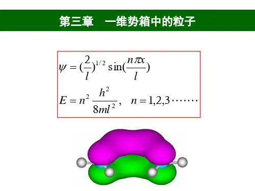
一维定态问题的薛定谔方程可以写成如下的形式：
$$-
\frac{\hbar^{2}}{2m}\frac{d^{2}\Psi(x)}{dx^{2}}+V(x)\Psi(x)=E \Psi(x)$$
其中，$\hbar$为约化普朗克常数，m为粒子的质量，V(x)为粒子在x位置处的势能，E为粒子的总能量，$\Psi(x)$为描述粒子波函数的解析函数。

一维定态问题中，由于波函数只与一个坐标x有关，因此我们可以采用分离变量的方法将波函数表示为如下形式：
$$\Psi(x)=\psi(x)e^{ikx}$$
其中，$\psi(x)$为关于x的解析函数，k为波矢。

将上式代入薛定谔方程，可将其简化为如下形式：
$$-\frac{\hbar^{2}}{2m}\psi''(x)+(V(x)-E)\psi(x)=0$$
这个简化后的方程可以通过求解得到波函数的解析表达式及对应的能量。

对于有限区域内的粒子，我们需要根据边界条件来限定波函数的形状，在定态问题中，我们通常采用周期性边界条件或硬壳边界条件。

通过分析一维定态问题的波函数和能谱，我们可以深入理解原子、分子、固体等复杂体系中微观粒子的行为规律，同时也可以为设计新的材料、光电子器件等提供理论基础和指导。

固体物理英语固体物理基本词汇（汉英对照）一画一维晶格 One-dimensional crystal lattice一维单原子链 One-dimensional monatomic chain 一维双原子链 One-dimensional diatomic chain 一维复式格子One-dimensional compound lattice 二画二维晶格 Two-dimensional crystal lattice二度轴 Twofold axis二度对称轴 Twofold axis of symmetry几何结构因子 Geometrical structure factor三画三斜晶系 Triclinic system三方晶系 Trigonal system三斜晶系 Triclinic system刃位错 Edge dislocation小角晶界 Low angle grain boundary马德隆常数 Madelung constant四画元素晶体 Element crystal元素的电负性 Electronegativities of elements元素的电离能 Ionization energies of the elements 元素的结合能 Cohesive energies of the elements 六方密堆积 Hexagonal close-packed六方晶系 Hexagonal system反演 Inversion分子晶体 Molecular Crystal切变模量 Shear module双原子链 Diatomic linear chain介电常数 Dielectric constant化学势 Chemical potential内能 Internal energy分布函数 Distribution function夫伦克耳缺陷 Frenkel defect比热 Specific heat中子散射 Neutron scattering五画布喇菲格子 Bravais lattice布洛赫函数 Bloch function布洛赫定理 Bloch theorem布拉格反射 Bragg reflection布里渊区 Brillouin zone布里渊区边界 Brillouin zone boundary 布里渊散射 Brillouin scattering正格子 Direct lattice正交晶系 Orthorhombic crystal system正则振动 Normal vibration正则坐标 Normal coordinates立方晶系 Cubic crystal system立方密堆积 Cubic close-packed四方晶系 Tetragonal crystal system对称操作 Symmetry operation对称群 Symmetric group正交化平面波 Orthogonalized plane wave电子-晶格相互作用 Electron-lattice interaction 电子热容量 Electronic heat capacity电阻率 Electrical resistivity电导率 Conductivity电子亲合势 Electron affinity电子气的动能 Kinetic energy of electron gas 电子气的压力 Pressure of electron gas电子分布函数 Electron distribution function 电负性 Electronegativity电磁声子 Electromagnetic phonon功函数 Work function长程力 Long-range force立方晶系 Cubic system平面波方法 plane wave method平移对称性 Translation symmetry平移对称操作 Translation symmetry operator 平移不变性 Translation invariance石墨结构 Graphite structure闪锌矿结构 Blende structure六画负电性 Electronegativity共价结合 Covalent binding共价键 Covalent bond共价晶体 Covalent crystals共价键的饱和 Saturation of covalent bonds 光学模 Optical modes光学支 Optical branch光散射 Light scattering红外吸收 Infrared absorption压缩系数 Compressibility扩散系数 Diffusion coefficient扩散的激活能 Activation energy of diffusion 共价晶体 Covalent Crystal价带 Valence band导带 Conduction band自扩散 Self-diffusion有效质量 Effective mass有效电荷 Effective charges弛豫时间 Relaxation time弛豫时间近似 Relaxation-time approximation扩展能区图式 Extended zone scheme自由电子模型 Free electron model自由能 Free energy杂化轨道 Hybrid orbit七画纯金属 Ideal metal体心立方 Body-centered cubic体心四方布喇菲格子 Body-centered tetragonal Bravais lattices 卤化碱晶体 Alkali-halide crystal劳厄衍射 Laue diffraction间隙原子 Interstitial atom间隙式扩散 Interstitial diffusion肖特基缺陷 Schottky defect位错 Dislocation滑移 Slip晶界 Grain boundaries伯格斯矢量 Burgers vector杜隆-珀替定律 Dulong-Petit’s law粉末衍射 Powder diffraction里查孙-杜师曼方程 Richardson-Dushman equation 克利斯托夫方程 Christofell equation克利斯托夫模量Christofell module位移极化 Displacement polarization声子 Phonon声学支 Acoustic branch应力 Stress 应变 Strain切应力 Shear stress切应变 Shear strain八画周期性重复单元 Periodic repeated unit底心正交格子 Base-centered orthorhombic lattice 底心单斜格工 Base-centered monoclinic lattices 单斜晶系 Monoclinic crystal system金刚石结构 Diamond structure金属的结合能 Cohesive energy of metals金属晶体 Metallic Crystal转动轴 Rotation axes转动-反演轴 Rotation-inversion axes转动晶体法 Rotating crystal method空间群 Space group空位 Vacancy范德瓦耳斯相互作用 Van der Waals interaction 金属性结合 Metallic binding单斜晶系 Monoclinic system单电子近似 Single-erection approximation极化声子 Polarization phonon拉曼散射 Raman scattering态密度 Density of states铁电软模 Ferroelectrics soft mode空穴 Hole万尼尔函数 Wannier function平移矢量 Translation vector非谐效应 Anharmonic effect周期性边界条件 Periodic boundary condition九画玻尔兹曼方程 Boltzman equation点群 Point groups迪. 哈斯－范. 阿耳芬效应 De Hass－Van Alphen effect胡克定律Hooke’s law氢键 Hydrogen bond亲合势 Affinity重迭排斥能 Overlap repulsive energy结合能 Cohesive energy玻恩-卡门边界条件 Born-Karman boundary condition费密-狄喇克分布函数 Fermi-Dirac distribution function费密电子气的简并性 Degeneracy of free electron Fermi gas 费密 Fermi费密能 Fermi energy费密能级 Fermi level费密球 Fermi sphere费密面 Fermi surface费密温度 Fermi temperature费密速度 Fermi velocity费密半径 Fermi radius恢复力常数 Constant of restorable force绝热近似 Adiabatic approximation十画原胞 Primitive cell原胞基矢 Primitive vectors倒格子 Reciprocal lattice倒格子原胞 Primitive cell of the reciprocal lattice 倒格子空间 Reciprocal space倒格点 Reciprocal lattice point倒格子基矢Primitive translation vectors of the reciprocal lattice倒格矢 Reciprocal lattice vector倒逆散射 Umklapp scattering粉末法 Powder method原子散射因子 Atomic scattering factor配位数 Coordination number原子和离子半径 Atomic and ionic radii原子轨道线性组合 Linear combination of atomic orbits离子晶体的结合能 Cohesive energy of inert crystals离解能 Dissociation energy离子键 Ionic bond离子晶体 Ionic Crystal离子性导电 Ionic conduction洛伦兹比 Lorenz ratio魏德曼－佛兰兹比 Weidemann－Franz ratio 缺陷的迁移 Migration of defects缺陷的浓度 Concentrations of lattice defects 爱因斯坦 Einstein爱因斯坦频率 Einstein frequency爱因斯坦温度 Einstein temperature格波 Lattice wave格林爱森常数 Gruneisen constant索末菲理论 Sommerfeld theory热电子发射 Thermionic emission热容量 Heat capacity热导率 Thermal conductivity热膨胀 Thermal expansion能带 Energy band能隙 Energy gap能带的简约能区图式 Reduced zone scheme of energy band 能带的周期能区图式 Repeated zone scheme of energy band 能带的扩展能区图式 Extended zone scheme of energy band 配分函数 Partition function准粒子 Quasi- particle准动量 Quasi- momentum准自由电子近似 Nearly free electron approximation十一画第一布里渊区 First Brillouin zone密堆积 Close-packing密勒指数 Miller indices接触电势差 Contact potential difference基元 Basis基矢 Basis vector弹性形变 Elastic deformation排斥能Repulsive energy弹性波 Elastic wave弹性应变张量 Elastic strain tensor弹性劲度常数 Elastic stiffness constant弹性顺度常数 Elastic compliance constant 弹性模量 Elastic module弹性动力学方程 Elastic-dynamics equation 弹性散射 Elastic scattering十二画等能面 Constant energy surface晶体 Crystal晶体结构 Crystal structure晶体缺陷 Crystal defect晶体衍射 Crystal diffraction晶列 Crystal array晶面 Crystal plane晶面指数 Crystal plane indices晶带 Crystal band晶向 direction晶格 lattice晶格常数 Lattice constant晶格周期势 Lattice-periodic potential 晶格周期性 Lattice-periodicity晶胞 Cell, Unit cell晶面间距 Interplanar spacing晶系 Crystal system晶体 Crystal晶体点群 Crystallographic point groups晶格振动 Latticevibration晶格散射 Lattice scattering散射 Scattering等能面 surface of constant energy十三画隋性气体晶体的结合能 Cohesive energy of inert gas crystals 滑移 Slip滑移面 Slip plane简单立方晶格 Simple cubic lattice简单晶格 Simple lattice简单单斜格子 Simple monoclinic lattice简单四方格子 Simple tetragonal lattice简单正交格子 Simple orthorhombic lattice简谐近似 Harmonic approximation简正坐标 Normal coordinates简正振动 Normal vibration简正模 Normal modes简约波矢 Reduced wave vector简约布里渊区 Reduced Brillouin zone禁带 Forbidden band紧束缚方法 Tight－binding method零点振动能 Zero-point vibration energy 雷纳德－琼斯势 Lenard－Jones potential 满带 Filled band十四画磁致电阻 Magnetoresistance模式密度 Density of modes漂移速度 Drift velocity漂移迁移率 Drift mobility十五至十七画德拜 Debye德拜近似 Debye approximation德拜截止频率 Debye cut-off frequency 德拜温度 Debye temperature霍耳效应 Hall effect螺位错 Screw dislocation赝势 Pseudopotential。

利用恒等式去计算积分
1 1 sin ni t sin n j t cos[( ni n j )t ] cos[( ni n j )t ] 2 2
j dx 于是： i *
2



0
1 2 1 cos[(ni n j )t ]dt cos[(ni n j )t ]dt 2 0 2
1/ 2
c2e
i ( 2mE )1 / 2 x /
(2mE) x /
II c1e c2e
i
i
由于：
e cos i sin
(c1 c2 ) cos i(c1 c2 ) sin A cos B sin
i
则： II c1 cos ic1 sin c2 cos ic2 sin
2
上述方程为常系数二阶线齐次方程，其辅助方程为：
s 2 2m E 2 0
此，上式可写为：
s 2mE
1
1
此处能量E为势能（为零）加上动能，所以为正的，因
s i 2mE
代入常系数二阶线齐次方程的通解公式，得：
II c1e
暂令： 则：
i ( 2mE )1 / 2 x /
1 1/ 2 1 1/ 2 A cos[ ( 2 mE ) x ] B sin[ ( 2 mE ) x] 于是： II
下面利用边界条件求任意常数A与B。
由于波函数是连续的，其值不会发生突跃。
若ψ在x=0点连续，则ψI和ψII在x=0处必趋于同一值，即：
lim I lim II
一维势箱波函数的正交归一性
对于一维势箱中特定的波函数Ψi，其量子数为ni，则：

eeee-
eeeeee-
eeeeeeeee-
eee-
e-
பைடு நூலகம்
electrons from ideal gas with charge e
Successes and problems of the Drude model
Successes: • explanation of electrical conductivity and thermal conductivity • Quantitative explanation of the Wiedemann-Franz law (by luck!) • The Hall effect and magnetoresistance • ac conductivity of metals Problems: • heat capacity puzzle: Classical particle: u = 3/2 nkBT, cv = 3/2 nkB = const., experiment cv ~ T • The susceptibility puzzle:
Sommerfeld model = Drude model + quantum mechanics = Free Electron Gas + Schrodinger equation + Fermi statistics
• Sommerfeld kept Drude’s concept of Free Electron Gas, and incorporate quantum mechanics into it. • Free Electron Gas model is also called Drude-Sommerfeld Model

第七章 能带结构分析
（二）参考阎守胜 3.8 面心立方晶胞含 3 个原子，设锌原子与铜原子之比为 m，则
n = (3 + 3m) / a3
kF3 = 3π 2n = 3(3 + 3m)π 2 a3
m
=
(akF )3
9π 2
−1
面心立方的倒格子为体心立方
⎧⎪a1 ⎪
=
a 2
(
j
+
k
)
⎪⎨a2 ⎪
=
a 2
k
=
= 2 k x2 2m1∗
+
=
2
k
2 y
2m2∗
整理有
kx2 2Em1∗
+
k
2 y
2Em2∗
=1
=2
=2
A(E)
=
π ab
=
π
2E =2
m1∗m2∗
ω
=
2π eB =2
dA( E
dE
)
=
2π eB =2
2π =2
m1∗m2∗ =
eB m1∗m2∗
7.6 如果电子的等能面方程为
4
( ) ( ) E k
( ) G
dk dt
=
−
1 =
G ev
G k
×
JG B
=
−e
⎛ ⎜
⎝
kx m1∗
G i+
ky m2∗
G j
⎞ ⎟
×
⎠
JG Bk′
写成分量形式，有
dkx dt
+
eBk y m2∗
=0
dk y dt
−

Boltzmann 方程 . . . . . . . . . . . . . . . . . . . . . . . . 碰撞算子 Q(f, f ) 的基本性质 . . . . . . . . . . . . . . . . . Fokker-Planck 方程、Landau 方程以及 Boltzmann 方程线性 化模型 . . . . . . . . . . . . . . . . . . . . . . . . . . . . . . Navier-Stokes 方程 . . . . . . . . . . . . . . . . . . . . . . . Gevrey 函数空间 . . . . . . . . . . . . . . . . . . . . . . . .
研究现状及本文主要结果 . . . . . . . . . . . . . . . . . . . . . . . 1.2.1 1.2.2 1.2.3 1.2.4 存在性及唯一性 . . . . . . . . . . . . . . . . . . . . . . . . . 动力学方程的正则性理论: 空间齐次情形 . . . . . . . . . . . 动力学方程的正则性理论: 空间非齐次情形 . . . . . . . . . . Navier-Stokes 方程的正则性理论 . . . . . . . . . . . . . . .
第二章 预备知识 2.1 2.2 2.3 基本记号
Fourier 变换 . . . . . . . . . . . . . . . . . . . . . . . . . . . . . . . 基本函数空间及常用不等式 . . . . . . . . . . . . . . . . . . . . . . 2.3.1 2.3.2 Lp 空间及其性质 . . . . . . . . . . . . . . . . . . . . . . . . Sobolev 空间及其性质 . . . . . . . . . . . . . . . . . . . . .

河南教育学院物理系
第五章指出：定域系统和满足经典极限条件的玻 色（费米）系统都遵从玻耳兹曼分布。按照统计 思想，宏观量是对应微观量的统计平均值，根据 等概率原理，这两类系统玻耳兹曼分布出现的概 率最大，其他分布实际上不出现，所以对这两类 系统，宏观量是玻耳兹曼分布下微观量的统计平 均值。本章根据玻耳兹曼分布讨论这两类系统的 热力学性质。
即
U N ln Z1
此式即内能的统计表达式
§6.1 热力学量的统计表达式
二、广义力的统计表达式 1. 外界对系统的广义力 系统在准静态元过程中，当外参量y变化dy时，外 dW Ydy 界对系统的功为
Y是与外参量y对应的外界对系统的广义作用力 例如：系统在准静态元过程中体积变化dV时，外 界的功为–pdV。广义力是压强。 2.广义微观力
遵从玻耳兹曼分布的系统的内能为
U al l l l e l
l l
e
l e l l
本式求和在粒子的能级和简并度知道后就能计算
§6.1 热力学量的统计表达式
为了方便，引入粒子配分函数Z1
本章主要内容 玻耳兹曼统计的热力学量表达式 玻耳兹曼统计的统计公式的应用 理想气体的物态方程，理想气体的内能和热的分布公式的应用 麦克斯韦速度分布律，能量均分定律， 两者的应用
§6.1 热力学量的统计表达式
本节根据玻耳兹曼分布推导热力学量的统计表 达式。要解决的问题：宏观量（如：热力学基 本函数）与玻耳兹曼分布的联系。我们根据宏 观量是微观量的统计平均值去寻找联系。 一、内能的统计表达式 内能是系统中粒子无规则运动总能量的统计平 均值
(dU Ydy ) Nd ln Z1 ln Z1

( M 1 N )! ( M 1)!N !
上一内容
下一内容 回主目录 返回
2017/3/19
(5) 将N个不同的物体放入M个不同容器 中(每个容器的容量不限) ，则： 第一个物体有M种放法 第二个物体有M种放法 MN ……………………… 第N个物体有M种放法
(6) 将N个不同的物体分成k份，要保证： 第一份：n1个 第二份：n2个 …………… 第 k 份：nk个
上一内容
下一内容 回主目录 返回
2017/3/19
•一、微态的粒子数目与能级的粒子数目
• • • • • • • •
1.微态、微态的能量、微态的粒子数 微态也称量子状态或量子态，是某一个粒子所处的状态。 微态的能量：处在该微态上粒子具有的能量，用j表示。 微态的粒子数：处在同一量子态的粒子的数目，用nj表示。 对总粒子数为N，体积为V，能量为U的系统有： N=nj ，U=nj j 2.能级、能级的粒子数目 能级：不同的量子态可能有相同的能量，我们称具有相同能 量的粒子是处于同一能级。能级的能量用i表示。 • 能级的粒子数目：具有相同能量的粒子数目，用ni表示。 • 对总粒子数为N，体积为V，能量为U的系统有： • N=ni ，U=ni i
上一内容
下一内容 回主目录 返回
2017/3/19
• 五、一维谐振子（双原子分子） • 双原子分子的振动可以分解为沿化学键方向伸缩振动和垂 直于化学键方向的振动，可看成独立的。 • 一维谐振子能级能量： v=（v+1/2）h • 一维谐振子简并度: gr,i=1 • v=0,1,2,3自然数 , 谐振子振动频率. • 基态能级: v,0=(1/2)h • 第一激发态能级: v,1 =(3/2)h • 10-11J，/kT1010不能用经典热力学方法处理 • 六、电子、核运动 • 没有统一公式 • 电子与核运动的能级差很大， e > 102 kT n 更大 • 一般处于基态且 ge,0=常数 gn,0=常数，所以不讨论。

弗兰克扬定律引言弗兰克扬定律（Frankl-Yang equation）通常用于描述一维非稳态热传导的现象，被广泛应用于材料科学和工程领域。

该定律由奥地利科学家欧仁·弗兰克尔（Eugene Frankl）和美国科学家陈景隆（Hao-Chi Chen）独立提出，并由美国工程师楊恩·楊（Yen Yen Yang）于1948年推广使用。

一级标题二级标题一三级标题一弗兰克扬定律的基本形式为：q=−k⋅dT dx其中，q表示单位时间内单位面积传导热量，k为热导率，T为温度，x为位置。

该方程表达了热传导过程中温度梯度和热流强度之间的关系。

三级标题二该定律适用于一维情况下的非稳态热传导问题，其中温度变化随时间和位置而变化。

在稳态情况下，温度不随时间变化，此时弗兰克扬定律简化为：q=−k⋅dT dx三级标题三弗兰克扬定律的应用范围广泛，例如在材料科学中用于研究材料的热导性能，在工程领域用于设计散热系统和热电器件等。

通过定量描述热传导过程，可以优化材料和设备的性能，提高能源利用效率。

三级标题四下面将介绍一些应用弗兰克扬定律的实例。

二级标题二三级标题一实例一：材料热导率测量弗兰克扬定律可以用于测量材料的热导率。

通过测量材料间的温度梯度和传导热流强度，可以利用弗兰克扬定律反推得到材料的热导率。

三级标题二实例二：热电器件设计弗兰克扬定律在热电器件设计中也发挥着重要作用。

热电器件可以将热能转化为电能或者反过来，其效率受到热传导的影响。

通过合理设计热传导路径和选择合适的材料，可以提高热电器件的效率。

三级标题三实例三：散热系统设计在电子设备中，散热系统的设计对保持设备的正常运行非常重要。

弗兰克扬定律可以用于分析散热系统中的热传导过程，优化散热系统的结构和材料，提高散热效率。

三级标题四实例四：地热能利用地热能是一种可再生能源，通过地下的热传导可以获取到地球的热能。

弗兰克扬定律可以用于描述地热能的传导过程，帮助设计高效的地热能利用系统。

４６ ５
江 西 师 范 大学 学报 （ 自然 科 学 版 ）
２ １ 钲 ０１
如果它 满足离 散形式 的 多辛守恒 律
ｄ
ห้องสมุดไป่ตู้
其 亿／ （ ＋ ＋ ＋ ＋ ， ＋ ， 中 １ ２ ０ ０ １ ０ ｏ ｌ ／ ＝ ２ ｌ １ ＋ ＋
ｌ ８ ／＝ ＋Ｏ ／ 等． ／ ２ （ ￣） ， ｏ ２ 消去引进的正则动量
ｑ — ｐ】 — ｐ ＝ ０ ｔ 。 ｃ ，
（ ｚ ： （一＋ ， ＋ ） 亿 ：， ，十 ）
其 中 ， 分别 是 方 向的 ２阶 中心差商 ：
＋ ， 一 ， ＋ １ｋ ２ ｋ
＝
，
一
（ ６ ）
Ｐｔ ｑ 一ｑ ｙ ０ — ｙ ．
引入正 则动 量 Ｐ ＝Ｄｑ ＝国 Ｐ ， ＝ 从 而得 到 ， ， ＝ ｑ ， 多辛 哈密尔顿 形式
，
｛ ｆＹ ＝ ， Ｐ— ｙ ０
（） ８
【 ＝ ｑ＝ ， ，
（＝（ ｙ． ｚ ＋２ ） ）
这是 标 准 的 １维线 性 薛定 谔方 程 的 多辛 结构 ，
示“ Ｙ，） （ ｎ的近似， ， ｔ 为简单起见， 也把它记成
材
，
＝ Ｕ
０
，
０，
更 一般 地，￣ Ｕ ｎｙ Ｊ ＋
看 ，这 种格 式 能 够快 速 地 模拟 原 问题 ，而且 守恒 性
ｆ （ ＋ ｗ ＝ ， ＝［ ２】 ［ ２］ ＞ ， ｉ ） ０ ）∈ 一 ， ０ ｎ ×０ 兀 ｔ ０ ， ， ，
｛ Ｙ） ＋．Ｙ＝ Ｙ２） 【 ， ，２ ， ， ， ，） ），） ＋， ｆ ｎ ｆ ０＝
，
ｌ ２ 一 ／
１２ ／

关键词: 量子自旋链；矩阵乘积态；拓扑序；Mott绝缘体
中图分类号：O41 文献标识码： A
目录
I. 引言
II. 一维量子自旋链体系概述 A. Haldane猜想 1. 一维反铁磁海森堡模型的低能有效理论 2. Lieb-Schultz-Mattis定理 B. 基于投影算符的严格可解量子自旋链模型 1. Majumdar-Ghosh模型 2. Affleck-Kennedy-Lieb-Tasaki模型 C. 矩阵乘积态 1. VBS态的矩阵乘积形式 2. 转移矩阵方法
16
3
1. 基态波函数的构造
16
4
2. SO(4)矩阵乘积态：自旋–轨道价键晶体
17
5
D. 一维SO(n)对称的双线性–双二次模型
18
5
E. 本章小结
20
6
8
8 IV. 拓扑不等价的VBS态及其对应的哈密顿量
20
9
A. VBS态的一般构造方式
20
1. 矩阵乘积态表示
20
10
2. 对应的哈密顿量
21
10
III. 一维SO(n)对称的严格可解量子自旋链模型 A. SO(n)李代数的数学背景 1. 矢量表示与Cartan-Weyl形式 2. 矢量表示的直积分解 B. SO(2l + 1)情形：新的Haldane能隙态
Received date: 2011-07-19 *gmzhang@
量子关联多体系统中的一个重要领域是对量子 自旋系统的研究。早在量子力学建立初期的1931年， Bethe就 对 一 维 量 子 自 旋1/2反 铁 磁 海 森 堡 链 进 行 了 研究[1]，开辟了量子自旋链研究的篇章。 对于高维 情形下的反铁磁体，Anderson等人在五十年代发展了 自旋波理论[2,3]， 预言了高维的反铁磁海森堡模型具 有长程序，低能元激发为无能隙的自旋波模式。 然 而，Mermin-Wagner-Coleman定理[4,5]指出，即使在零 温，量子涨落也会禁止一维具有连续对称性的体系中 产生反铁磁长程序。 这使得一维量子自旋系统中可能 存在许多不同寻常的物理。

1.1 问题背景 . . . . . . . . . . . . . . . . . . . . . . . . . . . . . . . . . . . . . . . . . . . . . . . . . . . . . . . . . . . . . . . . . . . . . . . . . . . 1 1.2 研究现状 . . . . . . . . . . . . . . . . . . . . . . . . . . . . . . . . . . . . . . . . . . . . . . . . . . . . . . . . . . . . . . . . . . . . . . . . . . . 4 1.3 研究内容 . . . . . . . . . . . . . . . . . . . . . . . . . . . . . . . . . . . . . . . . . . . . . . . . . . . . . . . . . . . . . . . . . . . . . . . . . . . 5 1.3.1 1.3.2 1.3.3 快速高效数值方法及其应用 . . . . . . . . . . . . . . . . . . . . . . . . . . . . . . . . . . . . . . . . . . . . . . . . 5 两类紧致差分格式的最优误差估计 . . . . . . . . . . . . . . . . . . . . . . . . . . . . . . . . . . . . . . . . 6 各向异性外势下三维方程组的降维分析 . . . . . . . . . . . . . . . . . . . . . . . . . . . . . . . . . . . 6

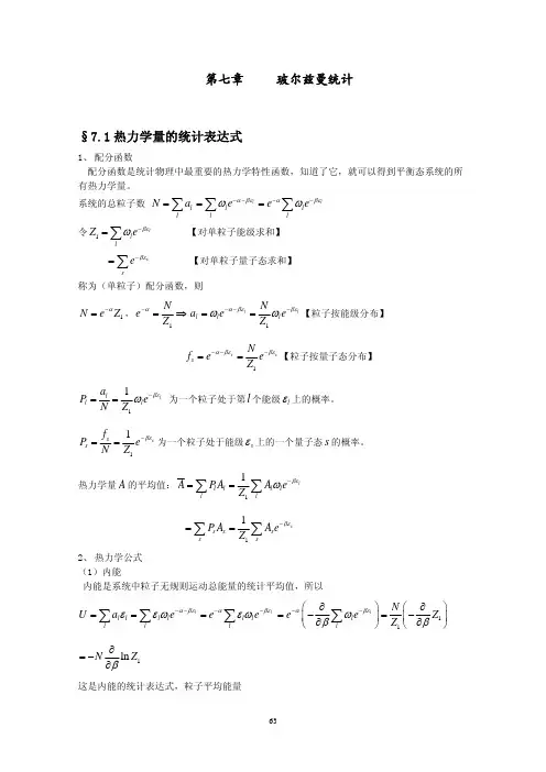
第七章玻耳兹曼统计7.1试根据公式-弓®务证明，对于非相对论粒子2处门 +；+£）,包，竹，吆=0,±1,±2,…）,其中V = L 3是系统的体积，常量凹力（〃；+圧+扇），并以单一指标/代表2m5 n y ,冬三个量子数. 由式（2）可得代入压强公式，有l 6习 2 p 匕 _2U 厂-刁®丽=齐弓也一百式中（/周是系统的内能./上述证明示涉及分布匕｝的具体表达式，因此式（4）对玻耳兹曼分布、玻 色分布和费米分布都成立.前面我们利用粒子能暈木征值对体积V 的依赖关系直接求得了系统的压 强与内能的关系.式（4）也可以用其他方法证明.例如，按照统计物理的一 般程序，在求得玻耳兹曼系统的配分函数或玻色（费米）系统的巨配分函数2U p =——・ "3V上述结论对于玻耳兹曼分布、玻色分布和费米分布都成立•解：处在边长为L 的立方体中，非相对论粒子的能量本征值为_ 1 S = 2^（竽）何（①‘"、'吆=° 土匕 ±2,…）, 为书写简便起见，我们将上式简记为2s t =aV 亍，(1)(2)2m 2m (3)(4)后，根据热力学量的统计表达式可以求得系统的压强和内能，比较二者也可证明式(4).见式(7.2.5)和式(7.5.5)及王竹溪《统计物理学导论》§6.2 式(8)和§6.5式(8).将位力定理用于理想气体也可直接证明式(4),见第九章补充题2式(6).需要强调，式(4)只适用于粒子仅有平衡运动的情形.如果粒子还有其他的自由度，式(4)中的U仅指平动内能.7.2试根据公式p = 冬证明，对于相对论粒子厶—17有1 U上述结论对于玻耳兹曼分布、玻色分布和费米分布都成立.解：处在边长为厶的立方体中，极端相对论粒子的能量本征值为%心”：=C 翠佃+n； + n： )2 (E"，代=0,±1,±2,…),(1)用指标/表示量子数心化叫“表示系统的斫积，V = 可将上式简记为可=肿，(2)其中1a = 2 兀+ 用 +A?;)1・由此可得凹=_丄小/气(3) dV 3 3 V代入压强公式，得木题与7」题结果的差异来自能量木征值与体积V函数关系的不同. 式(4)对玻耳兹曼分布、玻色分布和费米分布都适用.(4)7.3当选择不同的能量零点时，粒子第/个能级的能量可以取为£或和以△表示二者之差，△ = £；-£,.试证明相应配分函数存在以下关系Z；=e存乙，并讨论由配分函数乙和Z；求得的热力学函数有何差别.解：当选择不同的能量零点时，粒子能级的能量可以取为可或£；=£,+△.显然能级的简并度不受能量零点选择的影响.相应的配分函数分别为乙=》©严，(1)IZ；壬严/=旷心乞3百叭/=严厶、(2) 故In Z* = InZ, -(3) 根据内能、压强和嫡的统计表达式(7.1.4), (7.1.7)和(7.1.13),容易证明L=U + NA, (4)p =°,(5)S、S, (6) 式中N是系统的粒子数.能量零点相差为△时，内能相差/V△是显然的.式(5) 和式(6)表明，压强和嫡不因能量零点的选择而异.其他热力学函数请读者自行考虑.值得注意的是，由式(7.1.3)知a = a _ 阻、所以q = 3｛严阴与a； = 3严肚是相同的.粒子数的最概然分布不因能量零点的选择而异.在分析实际问题时可以视方便选择能量的零点.7.4试证明，对于遵从玻耳兹曼分布的定域系统，嫡函数可以表示为S=_Nk》21nR,式中人是粒子处在量子态s的概率,(1)S 是对粒子的所有量子态求和・对于满足经典极限条件的非定域系统，爛的表达式有何不同？ 解：根据式（6.6.9）,处在能量为的量子态s 上的平均粒子数为以N 表示系统的粒子数，粒子处在量子态s 上的概率为P = ------- = ----- ・ 5N Z,(2)显然，几满足归一化条件 式中工是对粒子的所有可能的量子态求和.粒子的平均能量可以表示为 (4)根据式（7.1.13）,定域系统的爛为 S = Nk In Z.-p ——InZ.= Nk(lnZ|+0?) = M 》P 『(lnZ|+06) = _NR 》P 」nP,.最后一步用了式（2）,即'In P 、= —InZ 】一0£y ・(5) (6)式（5）的爛表达式是颇具启发性的.嫡是广延量，具有相加性.式（5）意味着一个粒子的爛等于它取决于粒子处在各个可能状态的概率 S叮如果粒子肯定处在某个状态厂，即Pf,粒子的爛等于零.反之，当粒 子可能处在多个微观状态时，粒子的爛大于零.这与爛是无序度的量度的理 解自然是一致的.如果换一个角度考虑，粒子的状态完全确定意味着我们对 它有完全的信息，粒子以一定的概率处在各个可能的微观状态意味着我们对题5还将证明，在正则系综理论中爛也有类似的表达式.沙农(Shannon)在更普遍的意义上引进了信息嫡的概念，成为通信理论的出发点.甄尼斯(Jaynes)提岀将爛当作统计力学的基木假设，请参看第九章补充题5.对于满足经典极限条件的非定域系统，式(7.1.13’)给出dS = Nk lnZ|-0——InZ, 一klnN!,k 60 丿上式可表为S=—M》^ln£+S(), (7)3其中S{}=-k\nN\ = -Nk{\nN因为f 严NP「将式(7)用人表出，并注意D严N、3可得S = -k》fWh+Nk.(8)S这是满足玻耳兹曼分布的非定域系统的嫡的一个表达式.请与习题8.2的结果比较.7.5因体含有A, B两种原子.试证明由于原子在晶体格点的随机分布引起的混合爛为N'S = k\n-；——(N机N(l_x)_j!=-Nk [x In x + (1 - x) In (1 - A )],其中N是总原子数，x是A原子的百分比，1-x是B原子的百分比.注意x<l, 上式给出的爛为正值.解：玻耳兹曼关系给岀物质系统某个宏观状态的爛与相应微观状态数。