The Space Density of Galaxy Peaks and the Linear Matter Power Spectrum

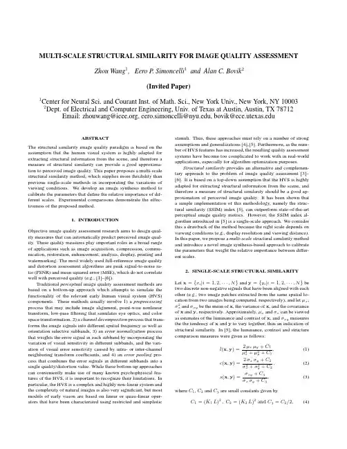
MULTI-SCALE STRUCTURAL SIMILARITY FOR IMAGE QUALITY ASSESSMENT Zhou Wang1,Eero P.Simoncelli1and Alan C.Bovik2(Invited Paper)1Center for Neural Sci.and Courant Inst.of Math.Sci.,New York Univ.,New York,NY10003 2Dept.of Electrical and Computer Engineering,Univ.of Texas at Austin,Austin,TX78712 Email:zhouwang@,eero.simoncelli@,bovik@ABSTRACTThe structural similarity image quality paradigm is based on the assumption that the human visual system is highly adapted for extracting structural information from the scene,and therefore a measure of structural similarity can provide a good approxima-tion to perceived image quality.This paper proposes a multi-scale structural similarity method,which supplies moreflexibility than previous single-scale methods in incorporating the variations of viewing conditions.We develop an image synthesis method to calibrate the parameters that define the relative importance of dif-ferent scales.Experimental comparisons demonstrate the effec-tiveness of the proposed method.1.INTRODUCTIONObjective image quality assessment research aims to design qual-ity measures that can automatically predict perceived image qual-ity.These quality measures play important roles in a broad range of applications such as image acquisition,compression,commu-nication,restoration,enhancement,analysis,display,printing and watermarking.The most widely used full-reference image quality and distortion assessment algorithms are peak signal-to-noise ra-tio(PSNR)and mean squared error(MSE),which do not correlate well with perceived quality(e.g.,[1]–[6]).Traditional perceptual image quality assessment methods are based on a bottom-up approach which attempts to simulate the functionality of the relevant early human visual system(HVS) components.These methods usually involve1)a preprocessing process that may include image alignment,point-wise nonlinear transform,low-passfiltering that simulates eye optics,and color space transformation,2)a channel decomposition process that trans-forms the image signals into different spatial frequency as well as orientation selective subbands,3)an error normalization process that weights the error signal in each subband by incorporating the variation of visual sensitivity in different subbands,and the vari-ation of visual error sensitivity caused by intra-or inter-channel neighboring transform coefficients,and4)an error pooling pro-cess that combines the error signals in different subbands into a single quality/distortion value.While these bottom-up approaches can conveniently make use of many known psychophysical fea-tures of the HVS,it is important to recognize their limitations.In particular,the HVS is a complex and highly non-linear system and the complexity of natural images is also very significant,but most models of early vision are based on linear or quasi-linear oper-ators that have been characterized using restricted and simplistic stimuli.Thus,these approaches must rely on a number of strong assumptions and generalizations[4],[5].Furthermore,as the num-ber of HVS features has increased,the resulting quality assessment systems have become too complicated to work with in real-world applications,especially for algorithm optimization purposes.Structural similarity provides an alternative and complemen-tary approach to the problem of image quality assessment[3]–[6].It is based on a top-down assumption that the HVS is highly adapted for extracting structural information from the scene,and therefore a measure of structural similarity should be a good ap-proximation of perceived image quality.It has been shown that a simple implementation of this methodology,namely the struc-tural similarity(SSIM)index[5],can outperform state-of-the-art perceptual image quality metrics.However,the SSIM index al-gorithm introduced in[5]is a single-scale approach.We consider this a drawback of the method because the right scale depends on viewing conditions(e.g.,display resolution and viewing distance). In this paper,we propose a multi-scale structural similarity method and introduce a novel image synthesis-based approach to calibrate the parameters that weight the relative importance between differ-ent scales.2.SINGLE-SCALE STRUCTURAL SIMILARITYLet x={x i|i=1,2,···,N}and y={y i|i=1,2,···,N}be two discrete non-negative signals that have been aligned with each other(e.g.,two image patches extracted from the same spatial lo-cation from two images being compared,respectively),and letµx,σ2x andσxy be the mean of x,the variance of x,and the covariance of x and y,respectively.Approximately,µx andσx can be viewed as estimates of the luminance and contrast of x,andσxy measures the the tendency of x and y to vary together,thus an indication of structural similarity.In[5],the luminance,contrast and structure comparison measures were given as follows:l(x,y)=2µxµy+C1µ2x+µ2y+C1,(1)c(x,y)=2σxσy+C2σ2x+σ2y+C2,(2)s(x,y)=σxy+C3σxσy+C3,(3) where C1,C2and C3are small constants given byC1=(K1L)2,C2=(K2L)2and C3=C2/2,(4)Fig.1.Multi-scale structural similarity measurement system.L:low-passfiltering;2↓:downsampling by2. respectively.L is the dynamic range of the pixel values(L=255for8bits/pixel gray scale images),and K1 1and K2 1aretwo scalar constants.The general form of the Structural SIMilarity(SSIM)index between signal x and y is defined as:SSIM(x,y)=[l(x,y)]α·[c(x,y)]β·[s(x,y)]γ,(5)whereα,βandγare parameters to define the relative importanceof the three components.Specifically,we setα=β=γ=1,andthe resulting SSIM index is given bySSIM(x,y)=(2µxµy+C1)(2σxy+C2)(µ2x+µ2y+C1)(σ2x+σ2y+C2),(6)which satisfies the following conditions:1.symmetry:SSIM(x,y)=SSIM(y,x);2.boundedness:SSIM(x,y)≤1;3.unique maximum:SSIM(x,y)=1if and only if x=y.The universal image quality index proposed in[3]corresponds to the case of C1=C2=0,therefore is a special case of(6).The drawback of such a parameter setting is that when the denominator of Eq.(6)is close to0,the resulting measurement becomes unsta-ble.This problem has been solved successfully in[5]by adding the two small constants C1and C2(calculated by setting K1=0.01 and K2=0.03,respectively,in Eq.(4)).We apply the SSIM indexing algorithm for image quality as-sessment using a sliding window approach.The window moves pixel-by-pixel across the whole image space.At each step,the SSIM index is calculated within the local window.If one of the image being compared is considered to have perfect quality,then the resulting SSIM index map can be viewed as the quality map of the other(distorted)image.Instead of using an8×8square window as in[3],a smooth windowing approach is used for local statistics to avoid“blocking artifacts”in the quality map[5].Fi-nally,a mean SSIM index of the quality map is used to evaluate the overall image quality.3.MULTI-SCALE STRUCTURAL SIMILARITY3.1.Multi-scale SSIM indexThe perceivability of image details depends the sampling density of the image signal,the distance from the image plane to the ob-server,and the perceptual capability of the observer’s visual sys-tem.In practice,the subjective evaluation of a given image varies when these factors vary.A single-scale method as described in the previous section may be appropriate only for specific settings.Multi-scale method is a convenient way to incorporate image de-tails at different resolutions.We propose a multi-scale SSIM method for image quality as-sessment whose system diagram is illustrated in Fig. 1.Taking the reference and distorted image signals as the input,the system iteratively applies a low-passfilter and downsamples thefiltered image by a factor of2.We index the original image as Scale1, and the highest scale as Scale M,which is obtained after M−1 iterations.At the j-th scale,the contrast comparison(2)and the structure comparison(3)are calculated and denoted as c j(x,y) and s j(x,y),respectively.The luminance comparison(1)is com-puted only at Scale M and is denoted as l M(x,y).The overall SSIM evaluation is obtained by combining the measurement at dif-ferent scales usingSSIM(x,y)=[l M(x,y)]αM·Mj=1[c j(x,y)]βj[s j(x,y)]γj.(7)Similar to(5),the exponentsαM,βj andγj are used to ad-just the relative importance of different components.This multi-scale SSIM index definition satisfies the three conditions given in the last section.It also includes the single-scale method as a spe-cial case.In particular,a single-scale implementation for Scale M applies the iterativefiltering and downsampling procedure up to Scale M and only the exponentsαM,βM andγM are given non-zero values.To simplify parameter selection,we letαj=βj=γj forall j’s.In addition,we normalize the cross-scale settings such thatMj=1γj=1.This makes different parameter settings(including all single-scale and multi-scale settings)comparable.The remain-ing job is to determine the relative values across different scales. Conceptually,this should be related to the contrast sensitivity func-tion(CSF)of the HVS[7],which states that the human visual sen-sitivity peaks at middle frequencies(around4cycles per degree of visual angle)and decreases along both high-and low-frequency directions.However,CSF cannot be directly used to derive the parameters in our system because it is typically measured at the visibility threshold level using simplified stimuli(sinusoids),but our purpose is to compare the quality of complex structured im-ages at visible distortion levels.3.2.Cross-scale calibrationWe use an image synthesis approach to calibrate the relative impor-tance of different scales.In previous work,the idea of synthesizing images for subjective testing has been employed by the“synthesis-by-analysis”methods of assessing statistical texture models,inwhich the model is used to generate a texture with statistics match-ing an original texture,and a human subject then judges the sim-ilarity of the two textures [8]–[11].A similar approach has also been qualitatively used in demonstrating quality metrics in [5],[12],though quantitative subjective tests were not conducted.These synthesis methods provide a powerful and efficient means of test-ing a model,and have the added benefit that the resulting images suggest improvements that might be made to the model[11].M )distortion level (MSE)12345Fig.2.Demonstration of image synthesis approach for cross-scale calibration.Images in the same row have the same MSE.Images in the same column have distortions only in one specific scale.Each subject was asked to select a set of images (one from each scale),having equal quality.As an example,one subject chose the marked images.For a given original 8bits/pixel gray scale test image,we syn-thesize a table of distorted images (as exemplified by Fig.2),where each entry in the table is an image that is associated witha specific distortion level (defined by MSE)and a specific scale.Each of the distorted image is created using an iterative procedure,where the initial image is generated by randomly adding white Gaussian noise to the original image and the iterative process em-ploys a constrained gradient descent algorithm to search for the worst images in terms of SSIM measure while constraining MSE to be fixed and restricting the distortions to occur only in the spec-ified scale.We use 5scales and 12distortion levels (range from 23to 214)in our experiment,resulting in a total of 60images,as demonstrated in Fig.2.Although the images at each row has the same MSE with respect to the original image,their visual quality is significantly different.Thus the distortions at different scales are of very different importance in terms of perceived image quality.We employ 10original 64×64images with different types of con-tent (human faces,natural scenes,plants,man-made objects,etc.)in our experiment to create 10sets of distorted images (a total of 600distorted images).We gathered data for 8subjects,including one of the authors.The other subjects have general knowledge of human vision but did not know the detailed purpose of the study.Each subject was shown the 10sets of test images,one set at a time.The viewing dis-tance was fixed to 32pixels per degree of visual angle.The subject was asked to compare the quality of the images across scales and detect one image from each of the five scales (shown as columns in Fig.2)that the subject believes having the same quality.For example,one subject chose the images marked in Fig.2to have equal quality.The positions of the selected images in each scale were recorded and averaged over all test images and all subjects.In general,the subjects agreed with each other on each image more than they agreed with themselves across different images.These test results were normalized (sum to one)and used to calculate the exponents in Eq.(7).The resulting parameters we obtained are β1=γ1=0.0448,β2=γ2=0.2856,β3=γ3=0.3001,β4=γ4=0.2363,and α5=β5=γ5=0.1333,respectively.4.TEST RESULTSWe test a number of image quality assessment algorithms using the LIVE database (available at [13]),which includes 344JPEG and JPEG2000compressed images (typically 768×512or similar size).The bit rate ranges from 0.028to 3.150bits/pixel,which allows the test images to cover a wide quality range,from in-distinguishable from the original image to highly distorted.The mean opinion score (MOS)of each image is obtained by averag-ing 13∼25subjective scores given by a group of human observers.Eight image quality assessment models are being compared,in-cluding PSNR,the Sarnoff model (JNDmetrix 8.0[14]),single-scale SSIM index with M equals 1to 5,and the proposed multi-scale SSIM index approach.The scatter plots of MOS versus model predictions are shown in Fig.3,where each point represents one test image,with its vertical and horizontal axes representing its MOS and the given objective quality score,respectively.To provide quantitative per-formance evaluation,we use the logistic function adopted in the video quality experts group (VQEG)Phase I FR-TV test [15]to provide a non-linear mapping between the objective and subjective scores.After the non-linear mapping,the linear correlation coef-ficient (CC),the mean absolute error (MAE),and the root mean squared error (RMS)between the subjective and objective scores are calculated as measures of prediction accuracy .The prediction consistency is quantified using the outlier ratio (OR),which is de-Table1.Performance comparison of image quality assessment models on LIVE JPEG/JPEG2000database[13].SS-SSIM: single-scale SSIM;MS-SSIM:multi-scale SSIM;CC:non-linear regression correlation coefficient;ROCC:Spearman rank-order correlation coefficient;MAE:mean absolute error;RMS:root mean squared error;OR:outlier ratio.Model CC ROCC MAE RMS OR(%)PSNR0.9050.901 6.538.4515.7Sarnoff0.9560.947 4.66 5.81 3.20 SS-SSIM(M=1)0.9490.945 4.96 6.25 6.98 SS-SSIM(M=2)0.9630.959 4.21 5.38 2.62 SS-SSIM(M=3)0.9580.956 4.53 5.67 2.91 SS-SSIM(M=4)0.9480.946 4.99 6.31 5.81 SS-SSIM(M=5)0.9380.936 5.55 6.887.85 MS-SSIM0.9690.966 3.86 4.91 1.16fined as the percentage of the number of predictions outside the range of±2times of the standard deviations.Finally,the predic-tion monotonicity is measured using the Spearman rank-order cor-relation coefficient(ROCC).Readers can refer to[15]for a more detailed descriptions of these measures.The evaluation results for all the models being compared are given in Table1.From both the scatter plots and the quantitative evaluation re-sults,we see that the performance of single-scale SSIM model varies with scales and the best performance is given by the case of M=2.It can also be observed that the single-scale model tends to supply higher scores with the increase of scales.This is not surprising because image coding techniques such as JPEG and JPEG2000usually compressfine-scale details to a much higher degree than coarse-scale structures,and thus the distorted image “looks”more similar to the original image if evaluated at larger scales.Finally,for every one of the objective evaluation criteria, multi-scale SSIM model outperforms all the other models,includ-ing the best single-scale SSIM model,suggesting a meaningful balance between scales.5.DISCUSSIONSWe propose a multi-scale structural similarity approach for image quality assessment,which provides moreflexibility than single-scale approach in incorporating the variations of image resolution and viewing conditions.Experiments show that with an appropri-ate parameter settings,the multi-scale method outperforms the best single-scale SSIM model as well as state-of-the-art image quality metrics.In the development of top-down image quality models(such as structural similarity based algorithms),one of the most challeng-ing problems is to calibrate the model parameters,which are rather “abstract”and cannot be directly derived from simple-stimulus subjective experiments as in the bottom-up models.In this pa-per,we used an image synthesis approach to calibrate the param-eters that define the relative importance between scales.The im-provement from single-scale to multi-scale methods observed in our tests suggests the usefulness of this novel approach.However, this approach is still rather crude.We are working on developing it into a more systematic approach that can potentially be employed in a much broader range of applications.6.REFERENCES[1] A.M.Eskicioglu and P.S.Fisher,“Image quality mea-sures and their performance,”IEEE munications, vol.43,pp.2959–2965,Dec.1995.[2]T.N.Pappas and R.J.Safranek,“Perceptual criteria for im-age quality evaluation,”in Handbook of Image and Video Proc.(A.Bovik,ed.),Academic Press,2000.[3]Z.Wang and A.C.Bovik,“A universal image quality in-dex,”IEEE Signal Processing Letters,vol.9,pp.81–84,Mar.2002.[4]Z.Wang,H.R.Sheikh,and A.C.Bovik,“Objective videoquality assessment,”in The Handbook of Video Databases: Design and Applications(B.Furht and O.Marques,eds.), pp.1041–1078,CRC Press,Sept.2003.[5]Z.Wang,A.C.Bovik,H.R.Sheikh,and E.P.Simon-celli,“Image quality assessment:From error measurement to structural similarity,”IEEE Trans.Image Processing,vol.13, Jan.2004.[6]Z.Wang,L.Lu,and A.C.Bovik,“Video quality assessmentbased on structural distortion measurement,”Signal Process-ing:Image Communication,special issue on objective video quality metrics,vol.19,Jan.2004.[7] B.A.Wandell,Foundations of Vision.Sinauer Associates,Inc.,1995.[8]O.D.Faugeras and W.K.Pratt,“Decorrelation methods oftexture feature extraction,”IEEE Pat.Anal.Mach.Intell., vol.2,no.4,pp.323–332,1980.[9] A.Gagalowicz,“A new method for texturefields synthesis:Some applications to the study of human vision,”IEEE Pat.Anal.Mach.Intell.,vol.3,no.5,pp.520–533,1981. [10] D.Heeger and J.Bergen,“Pyramid-based texture analy-sis/synthesis,”in Proc.ACM SIGGRAPH,pp.229–238,As-sociation for Computing Machinery,August1995.[11]J.Portilla and E.P.Simoncelli,“A parametric texture modelbased on joint statistics of complex wavelet coefficients,”Int’l J Computer Vision,vol.40,pp.49–71,Dec2000. [12]P.C.Teo and D.J.Heeger,“Perceptual image distortion,”inProc.SPIE,vol.2179,pp.127–141,1994.[13]H.R.Sheikh,Z.Wang, A. C.Bovik,and L.K.Cormack,“Image and video quality assessment re-search at LIVE,”/ research/quality/.[14]Sarnoff Corporation,“JNDmetrix Technology,”http:///products_services/video_vision/jndmetrix/.[15]VQEG,“Final report from the video quality experts groupon the validation of objective models of video quality assess-ment,”Mar.2000./.PSNRM O SSarnoffM O S(a)(b)Single−scale SSIM (M=1)M O SSingle−scale SSIM (M=2)M O S(c)(d)Single−scale SSIM (M=3)M O SSingle−scale SSIM (M=4)M O S(e)(f)Single−scale SSIM (M=5)M O SMulti−scale SSIMM O S(g)(h)Fig.3.Scatter plots of MOS versus model predictions.Each sample point represents one test image in the LIVE JPEG/JPEG2000image database [13].(a)PSNR;(b)Sarnoff model;(c)-(g)single-scale SSIM method for M =1,2,3,4and 5,respectively;(h)multi-scale SSIM method.。

高二英语天文辨析单选题40题1. Scientists have discovered that Mars has a much thinner atmosphere compared to Earth. Which of the following is a major consequence of this?A. It has a much weaker gravitational pullB. It has more extreme temperature variationsC. It has a shorter orbital periodD. It has no seasons答案解析：B。

首先分析A选项，行星的引力主要取决于其质量等因素，而不是大气厚度，所以A错误。

B选项，火星大气稀薄，不能很好地保存热量，导致昼夜和季节的温度变化非常极端，这是火星大气稀薄的一个重要结果，所以B正确。

C选项，火星的轨道周期是由其与太阳的距离等因素决定的，和大气厚度无关，C错误。

D选项，火星是有季节的，大气稀薄并不意味着没有季节，D错误。

2. Jupiter is known for its massive size. Which of the following statements about Jupiter's size is correct?A. Its diameter is about ten times that of EarthB. Its volume is exactly one thousand times that of EarthC. Its surface area is twice as large as all the other planets combinedD. Its mass is so large that it affects the orbits of all the inner planets答案解析：A。

高一英语宇宙探索单选题50题1. The _____ is a large system of stars, gas, and dust held together by gravity.A. planetB. galaxyC. moonD. comet答案：B。

本题考查宇宙探索中的基本词汇。

选项A“planet”（行星）是围绕恒星运行的天体，与题意不符；选项B“galaxy”（ 星系）是由恒星、气体和尘埃组成的巨大系统，由引力维系在一起，符合描述；选项C“moon”（ 月亮）是地球的卫星，只是一个小天体，不是这种大规模的系统；选项D“comet”（ 彗星）是一种特殊的天体，与星系的概念不同。

2. Scientists believe the universe _____ from a big bang.A. was originatedB. originatedC. has been originatedD. had originated答案：B。

本题考查宇宙起源相关的表达以及动词的用法。

“originate”表示“起源”，在这里是不及物动词，没有被动形式，所以选项A、C错误；选项D“had originated”是过去完成时，表示过去的过去，这里没有这种时间上的先后关系；选项B“originated”使用一般过去时，表达科学家认为宇宙起源于大爆炸这个过去的事实。

3. Which of the following is not a planet in our solar system?A. VenusB. SiriusC. MarsD. Jupiter答案：B。

本题考查太阳系中的行星知识和词汇。

选项A“Venus” 金星）、选项C“Mars” 火星）、选项D“ Jupiter” 木星）都是太阳系中的行星；而选项B“Sirius”（ 天狼星）是夜空中最亮的恒星，不是太阳系中的行星。

4. The sun is at the center of our _____.A. galaxyB. solar systemC. universeD. constellation答案：B。

高二英语天文积累单选题40题1. Mars is often called the "Red Planet" because of its ______.A. red soilB. red cloudsC. red oceansD. red mountains答案：A。

解析：火星被称为“红色星球”主要是因为其土壤呈现红色。

选项A“red soil”（ 红色土壤）符合火星的这一特征。

选项B“red clouds” 红色的云），火星的云不是使其被称为“红色星球”的主要原因。

选项C“red oceans”（ 红色的海洋），火星上并没有海洋。

选项D“red mountains” 红色的山脉），虽然火星有山脉，但不是整体被称为“红色星球”的主要因素。

2. Which planet has the largest number of moons in our solar system?A. MarsB. JupiterC. VenusD. Earth答案：B。

解析：在太阳系中，木星（Jupiter）拥有最多的卫星。

火星（Mars）的卫星数量较少。

金星（Venus）没有卫星。

地球（Earth）只有一颗卫星。

3. The orbit of ______ is between Mars and Saturn.A. JupiterB. VenusC. MercuryD. Neptune答案：A。

解析：木星 Jupiter）的轨道在火星 Mars）和土星Saturn）之间。

金星（Venus）的轨道在地球内侧。

水星（Mercury）是离太阳最近的行星，轨道在最内侧。

海王星（Neptune）的轨道在土星外侧。

4. Which planet has a very thick atmosphere mainly composed of carbon dioxide?A. MarsB. VenusC. EarthD. Jupiter答案：B。

试卷类型：A2024年深圳市高三年级第一次调研考试英 语2024. 2试卷共8页，卷面满分120分，折算成130分计入总分。

考试用时120分钟。

.注意事项：1.答题前，先将自己的姓名、准考证号填写在答题卡上，并将准考证号条形码粘贴在答题卡上的指定位置。

用2B铅笔将答题卡上试卷类型A后的方框涂黑。

2.选择题的作答：每小题选出答案后，用2B 铅笔把答题卡上对应题目的答案标号涂黑。

写在试题卷、草稿纸和答题卡上的非答题区域均无效。

3.非选择题的作答:用签字笔直接答在答题卡上对应的答题区域内。

写在试题卷、草稿纸和答题卡上的非答题区域均无效。

4.考试结束后，请将本试题卷和答题卡一并上交。

第二部分 阅读（共两节，满分50分)第一节（共15小题；每小题2. 5分，满分37. 5分）阅读下列短文，从每题所给的A、B、C、D四个选项中选出最佳选项。

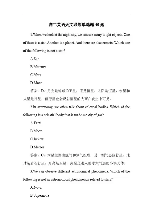
AWhistler Travel GuideSnow-capped peaks and powdered steeps; sparkling lakes and rushing waterfalls; challenging hiking routes and inviting restaurants—Whistler’s offerings suit every season.Things to doThe entire town displays the ski-chic atmosphere, hosting dozens of ski and snowboard competitions and festivals annually. In the warmer months, more outdoor enthusiasts come out to play. Visitors can try hiking or cycling up the mountains. While Whistle r is an ideal vacation spot for the active types, other travelers can enjoy the local museums and art galleries filled with informative exhibits. Plus, there are family-friendly activities and attractions like summer concerts, along with plenty of shopping options.When to visitThe best times to visit Whistler are from June through August and between December and March.How to get aroundThe best ways to get around Whistler are on foot or by bike. Or, you can take the shuttle buses from Whistler Village, which transport visitors to Lost Lake Park and the Marketplace. Meanwhile, having a car will allow you the freedom to explore top attractions like Whistler Train Wreck and Alexander Falls without having to spend a lot of cash on a cab.What you need to know● Whistler receives feet of snow each year. If you’re driving in winter, slow down and make sure to rent or come with a reliable SUV.● Snowslides are likely to occur on Backcountry routes, so only advanced skiers should take to this off-the-● Whistler’s wilderness is home to many black and grizzly bears. Keep your distance and do not feed them.21.What are active travelers recommended to do in Whistler?A. Bike up the mountains.B. Host ski competitions.C. Go shopping at the malls.D. Visit museum exhibitions.22.Which of the following is the most popular among travelers?A. Whistler Village.B. Lost Lake Park.C. The Marketplace.D. Whistler Train Wreck.23.What are travelers prohibited from doing in Whistler?A. Driving a rented SUV.B. Feeding grizzly bears.C. Exploring the wilderness.D. Skiing on Backcountry routes.BI used to believe that only words could catch the essence of the human soul. The literary works contained such distinct stories that they shaped the way we saw the world. Words were what composed the questions we sought to uncover and the answers to those questions themselves. Words were everything.That belief changed.In an ordinary math class, my teacher posed a simple question: What’s 0. 99 rounded to the nearest whole number? Easy. When rounded to the nearest whole number, 0. 99=1. Somehow, I thought even though 0. 99 is only 0. 01 away from 1, there’s still a 0. 01 difference. That means even if two things are only a little different, they are still different, so doesn’t that make them completely different?My teacher answered my question by presenting another equation (等式): 1 = 0. 9, which could also be expressed as 1=0. 999999… repeating itself without ever ending.There was something mysterious but fascinating about the equation. The left side was unchangeable, objective: it contained a number that ended. On the right was something endless, a number repeating itself limitless times. Yet, somehow, these two opposed things were connected by an equal sign.Lying in bed, I thought about how much the equation paralleled our existence. The left side of the equation represents that sometimes life itself is so unchangeable and so clear. The concrete, whole number of the day when you were born and the day when you would die. But then there is that gap in between life and death. The right side means a time and space full of limitless possibilities, and endless opportunities into the open future.So that’s what life is. Objective but imaginative. Unchangeable but limitless. Life is an equation with two sides that balances itself out. Still, we can’t ever truly seem to put the perfect words to it. So possibly numbers can express ideas as equally well as words can. For now, let’s leave it at that: 1 =0. 999999… and live a life like it.24.What does the author emphasize about words in paragraph 1?A. Their wide variety.B. Their literary origins.C. Their distinct sounds.D. Their expressive power.25.What made the author find the equation fascinating?A. The repetition of a number.B. The way two different numbers are equal.C. The question the teacher raised.D. The difference between the two numbers.26.Which of the following can replace the underlined word “paralleled” in paragraph 6?A. Measured.B. Composed.C. Mirrored.D. Influenced.A. The Perfect EquationB. Numbers Build EquationsC. An Attractive QuestionD. Words Outperform NumbersC“Why does grandpa have ear hair?” Just a few years ago my child was so curious to know “why” and “how” that we had to cut off her questions five minutes before bedtime. Now a soon-to-be fourth grader, she says that she dislikes school because “it’s not fun to learn. ”I am shocked. As a scientist and parent, I have done everything I can to promote a love of learning in my children. Where did I go wrong?My child’s experience is not unique. Developmental psychologist Susan Engel notes that curiosity —defined as “spontaneous(自发的) investigation and eagerness for new information”—drops dramatically in children by the fourth grade.In Wonder: Childhood and the Lifelong Love of Science, Yale psychologist Frank C. Keil details the development of wonder ——a spontaneous passion to explore, discover, and understand. He takes us on a journey from its early development, when wonder drives common sense and scientific reasoning, through the drop-off in wonder that often occurs, to the trap of life in a society that devalues wonder.As Keil notes, children are particularly rich in wonder while they are rapidly developing causal mechanisms(因果机制) in the preschool and early elementary school years. They are sensitive to the others’ knowledge and goals, and they expertly use their desire for questioning. Children’s questions, particularly those about “why” and “how, ” support the development of causal mechanisms which can be used to help their day-to-day reasoning.Unfortunately, as Keil notes, “adults greatly underestimate young children’s causal mechanisms. ”In the book, Wonder, Keil shows that we can support children’s ongoing wonder by playing games with them as partners, encouraging question-asking, and focusing on their abilities to reason and conclude.A decline in wonder is not unavoidable. Keil reminds us that we can accept wonder as a desirable positive quality that exists in everyone. I value wonder deeply, and Wonder has given me hope by proposing a future for my children that will remain wonder-full.28.What is a common problem among fourth graders?A. They upset their parents too often.B. They ask too many strange questions.C. Their love for fun disappears quickly.D. Their desire to learn declines sharply.29.What can be inferred about children’s causal mechanisms in paragraph 4?A. They control children’s sensitivity.B. They slightly change in early childhood.C. They hardly support children’s reasoning.D. They develop through children’s questioning.30.How can parents support children’s ongoing wonder according to Keil?A. By monitoring their games.B. By welcoming inquiring minds.C. By estimating their abilities.D. By providing reasonable conclusions.31.What is the text?A. A book review.B. A news report.C. A research paper.D. A children ‘s story.DEach year, the world loses about 10 million hectares of forest—an area about the size of Iceland because of cutting down trees. At that rate, some scientists predict the world’s forests could disappear in 100 to 200 years. To handle it, now researchers at Massachusetts Institute of Technology (MIT) have pioneered a technique to generateIn the lab, the researchers first take cells from the leaves of a young plant. These cells are cultured in liquid medium for two days, then moved to another medium which contains nutrients and two different hormones (激素). By adjusting the hormone levels, the researchers can tune the physical and mechanical qualities of the cells. Next, the researchers use a 3D printer to shape the cell-based material, and let the shaped material grow in the dark for three months. Finally, the researchers dehydrate(使脱水) the material, and then evaluate its qualities.They found that lower hormone levels lead to plant materials with more rounded, open cells of lower density(密度), while higher hormone levels contribute to the growth of plant materials with smaller but denser cell structures. Lower or higher density of cell structures makes the plant materials softer or more rigid, helping the materials grow with different wood-like characteristics. What’s more, it’s to be noted that the research process is about 100 times faster than the time it takes for a tree to grow to maturity!Research of this kind is ground-breaking. “This work demonstrates the great power of a technology, ”says lead researcher, Jeffrey Berenstain. “The real opportunity here is to be at its best with what you use and how you use it. This technology can be tuned to meet the requirements you give about shapes, sizes, rigidity, and forms. It enables us to ‘grow’ any wooden product in a way that traditional agricultural methods can’t achieve. ”32.Why do researchers at MIT conduct the research?A. To grow more trees.B. To protect plant diversity.C. To reduce tree losses.D. To predict forest disappearance.33.What does paragraph 2 mainly tell us about the lab research?A. Its theoretical basis.B. Its key procedures.C. Its scientific evidence.D. Its usual difficulties.34.What does the finding suggest about the plant materials?A. The hormone levels affect their rigidity.B. They are better than naturally grown plants.C. Their cells’ shapes mainly rely on their density.D. Their growth speed determines their characteristics.35.Why is the research ground-breaking according to Berenstain?A. It uses new biological materials in lab experiments.B. It revolutionizes the way to make wooden products.C. It challenges traditional scientific theories in forestry.D. It has a significant impact on worldwide plant growth.第二节（共5小题；每小题2. 5分，满分12. 5分）根据短文内容，从短文后的选项中选出能填入空白处的最佳选项。

小学上册英语第6单元期末试卷考试时间：100分钟（总分:120）A卷一、综合题(共计100题共100分)1. 听力题：A mixture can be separated by physical ______.2. 填空题：The _____ (猴子) is very curious and playful.3. 选择题：What do we call the force that pulls objects toward the Earth?A. MagnetismB. GravityC. FrictionD. Pressure答案: B4. 选择题：What do we call a young antelope?A. KidB. FawnC. CalfD. Pup答案:C. Calf5. 选择题：What do we call the act of setting goals?A. PlanningB. StrategyC. TargetingD. All of the Above答案：D6. 选择题：What do we call a small, fast-moving reptile?A. SnakeB. LizardC. CrocodileD. Turtle答案:B7. 填空题：The ________ has a colorful crown.8. 选择题：What do we call a person who studies ancient civilizations?A. HistorianB. ArchaeologistC. AnthropologistD. Paleontologist答案: B. Archaeologist9. 填空题：The ________ was a key event in the history of civil rights.10. 填空题：I can draw a picture of my favorite _________ (玩具) and share it with my class.11. 选择题：What is the name of the boy who never grows up?A. Peter PanB. Harry PotterC. PinocchioD. Aladdin12. 选择题：What is the color of a typical cloud?A. WhiteB. GrayC. BlueD. Green答案:A13. 填空题：The _____ (兔子) is known for its long ears.14. 填空题：The frog jumps from rock to ______.15. 填空题：I help my ______ with chores. (我帮我的______做家务。

小学上册英语第2单元真题试卷(有答案)英语试题一、综合题(本题有100小题，每小题1分，共100分.每小题不选、错误，均不给分)1.The ______ of a wave is the distance between two peaks.2.I enjoy ______ (参加) cultural events.3.I love to ______ (创造) new things.4.My brother has a toy ______ (赛车). He loves to race it on the ______ (地板).5. A ______ is a massive body of salt water.6.The ________ is very wise and lives in trees.7. A garden needs _______ to thrive.8.What do we call the place where we keep books?A. LibraryB. BookstoreC. ArchiveD. Museum答案:A9.The Milky Way galaxy is a spiral ______.10.The orca is a type of ________________ (鲸).11.My brother is a ______. He dreams of becoming a pilot.12.Martin Luther King Jr. fought for __________ (平等权利) for African Americans.13. A __________ is a large-scale geological event.14.My favorite color is the color of a ________.15.The _____ (lettuce) grows quickly in cool weather.16.The chemical formula for sodium acetate is _______.17.I like to go to ______ (展览) to see new art and ideas. It broadens my perspective.18.The capital of Antigua and Barbuda is ________ (圣约翰).19.The main component of natural gas is _____.20.The flower is very ___. (pretty)21. A ________ (植物景观设计) can transform spaces.22.Which of these animals can swim?A. DogB. BirdC. FishD. Lion答案:C Fish23. A _____ (秋天) walk reveals many colorful leaves.24.I think it’s important to be curious. Asking questions helps us learn and grow. I love discovering new facts about __________ and sharing them with my friends.25.我会连一连。

高二英语天文联想练习题50题(答案解析)1. The ______ is the largest planet in our solar system.A. EarthB. MarsC. JupiterD. Venus答案：C。

解析：本题考查太阳系中行星的相关知识以及词汇辨析。

A选项Earth是地球，不是太阳系中最大的行星；B选项Mars是火星，它比木星小；C选项Jupiter是木星，它是太阳系中最大的行星，符合题意；D选项Venus是金星，也不是最大的行星。

2. A ______ is a group of stars that forms a pattern in the sky.A. planetB. satelliteC. constellationD. meteor答案：C。

解析：本题考查天文术语的辨析。

A选项planet是行星，行星是独立的天体，不是一群星星组成的图案；B选项satellite 是卫星，围绕行星运转，和星星组成图案无关；C选项constellation 是星座，是天空中形成图案的一群星星，符合题意；D选项meteor是流星，不是星星组成的图案。

3. The ______ of the moon causes tides on Earth.A. lightB. gravityC. orbitD. surface答案：B。

解析：本题考查月球与地球之间的关系以及词汇辨析。

A选项light是光，月球的光不会引起地球的潮汐；B选项gravity是重力，月球的重力会引起地球的潮汐，这是基本的天文现象；C选项orbit是轨道，月球的轨道和地球的潮汐没有直接因果关系；D选项surface是表面，月球的表面与地球潮汐无关。

4. We can observe many ______ in the night sky, like the Milky Way.A. galaxiesB. asteroidsC. cometsD. nebulas答案：A。

关于宇宙太空的英语作文英文回答：The vast expanse of space has long captivatedhumanity's imagination, inspiring awe and wonder. Its mysteries have lured us to explore the cosmos, unlocking secrets that have profoundly shaped our understanding of our place in the universe.Space is a vacuum, devoid of matter in the form of molecules or gases. Within this vacuum, countless stars, planets, galaxies, and other celestial objects dance in an intricate ballet. The stars, like miniature suns, emittheir own light and energy, illuminating the cosmos with their brilliant glow. Planets, like our own Earth, orbit stars, reflecting their light and hosting diverse environments that support life. Galaxies, vast collections of stars, dust, and gas, contain billions of stars and span distances that defy comprehension.Our planet, Earth, is a pale blue dot in the vastness of space. It is a watery sphere, with oceans covering over 70% of its surface. Continents and islands rise above the water, forming diverse ecosystems that support a multitude of life forms. From the towering peaks of mountains to the depths of the oceans, Earth is a vibrant tapestry of interconnected life.Beyond Earth, our solar system is home to various planets, including Mercury, Venus, Mars, Jupiter, Saturn, Uranus, and Neptune. Each planet possesses unique characteristics, from scorching hot surfaces to swirling gas giants. The solar system also hosts numerous moons, comets, asteroids, and meteoroids, all orbiting the Sun in a harmonious dance.Our galaxy, the Milky Way, is a vast, spiral-shaped collection of stars, gas, and dust. It is estimated to contain hundreds of billions of stars, including our own Sun. The Milky Way is part of a larger cluster of galaxies known as the Local Group, which also includes the Andromeda Galaxy and other smaller galaxies.The universe is an immense and ever-expanding void, stretching far beyond the boundaries of our comprehension. Scientists believe that the universe originated from a single point, known as the Big Bang, approximately 13.8 billion years ago. Since then, the universe has been expanding and cooling, leading to the formation of stars, galaxies, and the countless objects that inhabit it.As we continue to explore the cosmos, we are confronted with its vastness and the mysteries that it holds. The search for life beyond Earth, the nature of dark matter and dark energy, and the ultimate fate of the universe are just a few of the questions that drive our insatiable curiosity.The study of space has not only expanded our knowledge of the cosmos but has also had profound implications for our lives on Earth. Satellites orbiting the planet provide us with communication, navigation, and weather forecasting capabilities. Space telescopes have revealed stunning images of distant galaxies, providing valuable insightsinto their evolution and composition. The exploration ofspace has also fostered international cooperation,inspiring nations to work together to advance our understanding of the universe.As we look up at the night sky, we are reminded of the vastness of the cosmos and the insignificance of our own existence. Yet, it is in this insignificance that we find our purpose. By studying the universe, we are not only unraveling its mysteries but also discovering more about ourselves and our place in the grand scheme of things.中文回答：一望无垠的太空自古以来就激发了人类的想象力，让人敬畏和惊叹。

高二英语天文积累单选题40题1. Scientists have found evidence of water on Mars in the past few years. Which of the following statements about Mars is correct?A. Mars has a thick atmosphere like Earth.B. Mars is the closest planet to the Sun.C. Mars has polar ice caps.D. Mars has no volcanoes.答案：C。

解析：选项A，火星的大气层非常稀薄，不像地球那样浓厚，所以A错误。

选项B，离太阳最近的行星是水星，不是火星，B错误。

选项C，火星有极地冰盖，这是已经被探测到的，C正确。

选项D，火星上有火山，D错误。

这道题主要考查关于火星的基本天文知识以及对相关词汇的理解。

2. Venus is often called Earth's "sister planet" because of its similar size. However, there are significant differences. Which one is a major difference?A. Venus has no mountains.B. Venus rotates in the opposite direction compared to most planets.C. Venus has a moon.D. Venus has a very cold surface.答案：B。

解析：选项A，金星有山脉，A错误。

选项B，金星与大多数行星相比，自转方向相反，这是它和地球的一个重要区别，B正确。

选项C，金星没有卫星，C错误。

选项D，金星表面温度非常高，而不是很冷，D错误。