Lecture 2 Strategic-form games

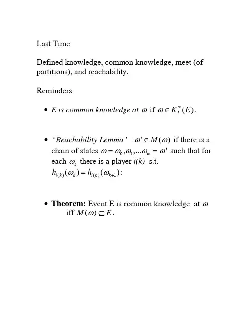
Last Time:Defined knowledge, common knowledge, meet (of partitions), and reachability.Reminders:• E is common knowledge at ω if ()I K E ω∞∈.• “Reachability Lemma” :'()M ωω∈ if there is a chain of states 01,,...m 'ωωωωω== such that for each k ω there is a player i(k) s.t. ()()1()(i k k i k k h h )ωω+=:• Theorem: Event E is common knowledge at ωiff ()M E ω⊆.How does set of NE change with information structure?Suppose there is a finite number of payoff matrices 1,...,L u u for finite strategy sets 1,...,I S SState space Ω, common prior p, partitions , and a map i H λso that payoff functions in state ω are ()(.)u λω; the strategy spaces are maps from into . i H i SWhen the state space is finite, this is a finite game, and we know that NE is u.h.c. and generically l.h.c. in p. In particular, it will be l.h.c. at strict NE.The “coordinated attack” game8,810,11,100,0A B A B-- 0,010,11,108,8A B A B--a ub uΩ= 0,1,2,….In state 0: payoff functions are given by matrix ; bu In all other states payoff functions are given by . a upartitions of Ω1H : (0), (1,2), (3,4),… (2n-1,2n)... 2H (0,1),(2,3). ..(2n,2n+1)…Prior p : p(0)=2/3, p(k)= for k>0 and 1(1)/3k e e --(0,1)ε∈.Interpretation: coordinated attack/email:Player 1 observes Nature’s choice of payoff matrix, sends a message to player 2.Sending messages isn’t a strategic decision, it’s hard-coded.Suppose state is n=2k >0. Then 1 knows the payoffs, knows 2 knows them. Moreover 2 knows that 1knows that 2 knows, and so on up to strings of length k: . 1(0n I n K n -Î>)But there is no state at which n>0 is c.k. (to see this, use reachability…).When it is c.k. that payoff are given by , (A,A) is a NE. But.. auClaim: the only NE is “play B at every information set.”.Proof: player 1 plays B in state 0 (payoff matrix ) since it strictly dominates A. b uLet , and note that .(0|(0,1))q p =1/2q >Now consider player 2 at information set (0,1).Since player 1 plays B in state 0, and the lowest payoff 2 can get to B in state 1 is 0, player 2’s expected payoff to B at (0,1) is at least 8. qPlaying A gives at most 108(1)q q −+−, and since , playing B is better. 1/2q >Now look at player 1 at 1(1,2)h =. Let q'=p(1|1,2), and note that '1(1)q /2εεεε=>+−.Since 2 plays B in state 1, player 1's payoff to B is at least 8q';1’s payoff to A is at most -10q'+8(1-q) so 1 plays B Now iterate..Conclude that the unique NE is always B- there is no NE in which at some state the outcome is (A,A).But (A,A ) is a strict NE of the payoff matrix . a u And at large n, there is mutual knowledge of the payoffs to high order- 1 knows that 2 knows that …. n/2 times. So “mutual knowledge to large n” has different NE than c.k.Also, consider "expanded games" with state space . 0,1,....,...n Ω=∞For each small positive ε let the distribution p ε be as above: 1(0)2/3,()(1)/3n p p n ee e e -==- for 0 and n <<∞()0p ε∞=.Define distribution by *p *(0)2/3p =,. *()1/3p ∞=As 0ε→, probability mass moves to higher n, andthere is a sense in which is the limit of the *p p εas 0ε→.But if we do say that *p p ε→ we have a failure of lower hemi continuity at a strict NE.So maybe we don’t want to say *p p ε→, and we don’t want to use mutual knowledge to large n as a notion of almost common knowledge.So the questions:• When should we say that one information structure is close to another?• What should we mean by "almost common knowledge"?This last question is related because we would like to say that an information structure where a set of events E is common knowledge is close to another information structure where these events are almost common knowledge.Monderer-Samet: Player i r-believes E at ω if (|())i p E h r ω≥.()r i B E is the set of all ω where player i r- believesE; this is also denoted 1.()ri B ENow do an iterative definition in the style of c.k.: 11()()rr I i i B E B E =Ç (everyone r-believes E) 1(){|(()|())}n r n ri i I B E p B E h r w w -=³ ()()n r n rI i i B E B =ÇEE is common r belief at ω if ()rI B E w ¥ÎAs with c.k., common r-belief can be characterized in terms of public events:• An event is a common r-truism if everyone r -believes it when it occurs.• An event is common r -belief at ω if it is implied by a common r-truism at ω.Now we have one version of "almost ck" : An event is almost ck if it is common r-belief for r near 1.MS show that if two player’s posteriors are common r-belief, they differ by at most 2(1-r): so Aumann's result is robust to almost ck, and holds in the limit.MS also that a strict NE of a game with knownpayoffs is still a NE when payoffs are "almost ck” - a form of lower hemi continuity.More formally:As before consider a family of games with fixed finite action spaces i A for each player i. a set of payoff matrices ,:l I u A R ->a state space W , that is now either finite or countably infinite, a prior p, a map such that :1,,,L l W®payoffs at ω are . ()(,)()w u a u a l w =Payoffs are common r-belief at ω if the event {|()}w l w l = is common r belief at ω.For each λ let λσ be a NE for common- knowledgepayoffs u .lDefine s * by *(())s l w w s =.This assigns each w a NE for the corresponding payoffs.In the email game, one such *s is . **(0)(,),()(,)s B B s n A A n ==0∀>If payoffs are c.k. at each ω, then s* is a NE of overall game G. (discuss)Theorem: Monder-Samet 1989Suppose that for each l , l s is a strict equilibrium for payoffs u λ.Then for any there is 0e >1r < and 1q < such that for all [,1]r r Î and [,1]q q Î,if there is probability q that payoffs are common r- belief, then there is a NE s of G with *(|()())1p s s ωωω=>ε−.Note that the conclusion of the theorem is false in the email game:there is no NE with an appreciable probability of playing A, even though (A,A) is a strict NE of the payoffs in every state but state 0.This is an indirect way of showing that the payoffs are never ACK in the email game.Now many payoff matrices don’t have strictequilibria, and this theorem doesn’t tell us anything about them.But can extend it to show that if for each state ω, *(s )ω is a Nash (but not necessarily strict Nash) equilibrium, then for any there is 0e >1r < and 1q < such that for all [,1]r r Î and [,1]q q Î, if payoffs are common r-belief with probability q, there is an “interim ε equilibria” of G where s * is played with probability 1ε−.Interim ε-equilibria:At each information set, the actions played are within epsilon of maxing expected payoff(((),())|())((',())|())i i i i i i i i E u s s h w E u s s h w w w w e-->=-Note that this implies the earlier result when *s specifies strict equilibria.Outline of proof:At states where some payoff function is common r-belief, specify that players follow s *. The key is that at these states, each player i r-believes that all other players r-believe the payoffs are common r-belief, so each expects the others to play according to s *.*ΩRegardless of play in the other states, playing this way is a best response, where k is a constant that depends on the set of possible payoff functions.4(1)k −rTo define play at states in */ΩΩconsider an artificial game where players are constrained to play s * in - and pick a NE of this game.*ΩThe overall strategy profile is an interim ε-equilibrium that plays like *s with probability q.To see the role of the infinite state space, consider the"truncated email game"player 2 does not respond after receiving n messages, so there are only 2n states.When 2n occurs: 2 knows it occurs.That is, . {}2(0,1),...(22,21,)(2)H n n =−−n n {}1(0),(1,2),...(21,2)H n =−.()2|(21,2)1p n n n ε−=−, so 2n is a "1-ε truism," and thus it is common 1-ε belief when it occurs.So there is an exact equilibrium where players playA in state 2n.More generally: on a finite state space, if the probability of an event is close to 1, then there is high probability that it is common r belief for r near 1.Not true on infinite state spaces…Lipman, “Finite order implications of the common prior assumption.”His point: there basically aren’t any!All of the "bite" of the CPA is in the tails.Set up: parameter Q that people "care about" States s S ∈,:f S →Θ specifies what the payoffs are at state s. Partitions of S, priors .i H i pPlayer i’s first order beliefs at s: the conditional distribution on Q given s.For B ⊆Θ,1()()i s B d =('|(')|())i i p s f s B h s ÎPlayer i’s second order beliefs: beliefs about Q and other players’ first order beliefs.()21()(){'|(('),('))}|()i i j i s B p s f s s B h d d =Îs and so on.The main point can be seen in his exampleTwo possible values of an unknown parameter r .1q q = o 2qStart with a model w/o common prior, relate it to a model with common prior.Starting model has only two states 12{,}S s s =. Each player has the trivial partition- ie no info beyond the prior.1122()()2/3p s p s ==.example: Player 1 owns an asset whose value is 1 at 1θ and 2 at 2θ; ()i i f s θ=.At each state, 1's expected value of the asset 4/3, 2's is 5/3, so it’s common knowledge that there are gains from trade.Lipman shows we can match the players’ beliefs, beliefs about beliefs, etc. to arbitrarily high order in a common prior model.Fix an integer N. construct the Nth model as followsState space'S ={1,...2}N S ´Common prior is that all states equally likely.The value of θ at (s,k) is determined by the s- component.Now we specify the partitions of each player in such a way that the beliefs, beliefs about beliefs, look like the simple model w/o common prior.1's partition: events112{(,1),(,2),(,1)}...s s s 112{(,21),(,2),(,)}s k s k s k -for k up to ; the “left-over” 12N -2s states go into 122{(,21),...(,2)}N N s s -+.At every event but the last one, 1 thinks the probability of is 2/3.1qThe partition for player 2 is similar but reversed: 221{(,21),(,2),(,)}s k s k s k - for k up to . 12N -And at all info sets but one, player 2 thinks the prob. of is 1/3.1qNow we look at beliefs at the state 1(,1)s .We matched the first-order beliefs (beliefs about θ) by construction)Now look at player 1's second-order beliefs.1 thinks there are 3 possible states 1(,1)s , 1(,2)s , 2(,1)s .At 1(,1)s , player 2 knows {1(,1)s ,2(,1)s ,(,}. 22)s At 1(,2)s , 2 knows . 122{(,2),(,3),(,4)}s s s At 2(,1)s , 2 knows {1(,2)s , 2(,1)s ,(,}. 22)sThe support of 1's second-order beliefs at 1(,1)s is the set of 2's beliefs at these info sets.And at each of them 2's beliefs are (1/3 1θ, 2/3 2θ). Same argument works up to N:The point is that the N-state models are "like" the original one in that beliefs at some states are the same as beliefs in the original model to high but finite order.(Beliefs at other states are very different- namely atθ or 2 is sure the states where 1 is sure that state is2θ.)it’s1Conclusion: if we assume that beliefs at a given state are generated by updating from a common prior, this doesn’t pin down their finite order behavior. So the main force of the CPA is on the entire infinite hierarchy of beliefs.Lipman goes on from this to make a point that is correct but potentially misleading: he says that "almost all" priors are close to a common. I think its misleading because here he uses the product topology on the set of hierarchies of beliefs- a.k.a topology of pointwise convergence.And two types that are close in this product topology can have very different behavior in a NE- so in a sense NE is not continuous in this topology.The email game is a counterexample. “Product Belief Convergence”:A sequence of types converges to if thesequence converges pointwise. That is, if for each k,, in t *i t ,,i i k n k *δδ→.Now consider the expanded version of the email game, where we added the state ∞.Let be the hierarchy of beliefs of player 1 when he has sent n messages, and let be the hierarchy atthe point ∞, where it is common knowledge that the payoff matrix is .in t ,*i t a uClaim: the sequence converges pointwise to . in t ,*i t Proof: At , i’s zero-order beliefs assignprobability 1 to , his first-order beliefs assignprobability 1 to ( and j knows it is ) and so onup to level n-1. Hence as n goes to infinity, thehierarchy of beliefs converges pointwise to common knowledge of .in t a u a u a u a uIn other words, if the number of levels of mutual knowledge go to infinity, then beliefs converge to common knowledge in the product topology. But we know that mutual knowledge to high order is not the same as almost common knowledge, and types that are close in the product topology can play very differently in Nash equilibrium.Put differently, the product topology on countably infinite sequences is insensitive to the tail of the sequence, but we know that the tail of the belief hierarchy can matter.Next : B-D JET 93 "Hierarchies of belief and Common Knowledge”.Here the hierarchies of belief are motivated by Harsanyi's idea of modelling incomplete information as imperfect information.Harsanyi introduced the idea of a player's "type" which summarizes the player's beliefs, beliefs about beliefs etc- that is, the infinite belief hierarchy we were working with in Lipman's paper.In Lipman we were taking the state space Ω as given.Harsanyi argued that given any element of the hierarchy of beliefs could be summarized by a single datum called the "type" of the player, so that there was no loss of generality in working with types instead of working explicitly with the hierarchies.I think that the first proof is due to Mertens and Zamir. B-D prove essentially the same result, but they do it in a much clearer and shorter paper.The paper is much more accessible than MZ but it is still a bit technical; also, it involves some hard but important concepts. (Add hindsight disclaimer…)Review of math definitions:A sequence of probability distributions converges weakly to p ifn p n fdp fdp ®òò for every bounded continuous function f. This defines the topology of weak convergence.In the case of distributions on a finite space, this is the same as the usual idea of convergence in norm.A metric space X is complete if every Cauchy sequence in X converges to a point of X.A space X is separable if it has a countable dense subset.A homeomorphism is a map f between two spaces that is 1-1, and onto ( an isomorphism ) and such that f and f-inverse are continuous.The Borel sigma algebra on a topological space S is the sigma-algebra generated by the open sets. (note that this depends on the topology.)Now for Brandenburger-DekelTwo individuals (extension to more is easy)Common underlying space of uncertainty S ( this is called in Lipman)ΘAssume S is a complete separable metric space. (“Polish”)For any metric space, let ()Z D be all probability measures on Borel field of Z, endowed with the topology of weak convergence. ( the “weak topology.”)000111()()()n n n X S X X X X X X --=D =´D =´DSo n X is the space of n-th order beliefs; a point in n X specifies (n-1)st order beliefs and beliefs about the opponent’s (n-1)st order beliefs.A type for player i is a== 0012(,,,...)()n i i i i n t X d d d =¥=δD0T .Now there is the possibility of further iteration: what about i's belief about j's type? Do we need to add more levels of i's beliefs about j, or is i's belief about j's type already pinned down by i's type ?Harsanyi’s insight is that we don't need to iterate further; this is what B-D prove formally.Coherency: a type is coherent if for every n>=2, 21marg n X n n d d --=.So the n and (n-1)st order beliefs agree on the lower orders. We impose this because it’s not clear how to interpret incoherent hierarchies..Let 1T be the set of all coherent typesProposition (Brandenburger-Dekel) : There is a homeomorphism between 1T and . 0()S T D ´.The basis of the proposition is the following Lemma: Suppose n Z are a collection of Polish spaces and let021201...1{(,,...):(...)1, and marg .n n n Z Z n n D Z Z n d d d d d --´´-=ÎD ´"³=Then there is a homeomorphism0:(nn )f D Z ¥=®D ´This is basically the same as Kolmogorov'sextension theorem- the theorem that says that there is a unique product measure on a countable product space that corresponds to specified marginaldistributions and the assumption that each component is independent.To apply the lemma, let 00Z X =, and 1()n n Z X -=D .Then 0...n n Z Z X ´´= and 00n Z S T ¥´=´.If S is complete separable metric than so is .()S DD is the set of coherent types; we have shown it is homeomorphic to the set of beliefs over state and opponent’s type.In words: coherency implies that i's type determines i's belief over j's type.But what about i's belief about j's belief about i's type? This needn’t be determined by i’s type if i thinks that j might not be coherent. So B-D impose “common knowledge of coherency.”Define T T ´ to be the subset of 11T T ´ where coherency is common knowledge.Proposition (Brandenburger-Dekel) : There is a homeomorphism between T and . ()S T D ´Loosely speaking, this says (a) the “universal type space is big enough” and (b) common knowledge of coherency implies that the information structure is common knowledge in an informal sense: each of i’s types can calculate j’s beliefs about i’s first-order beliefs, j’s beliefs about i’s beliefs about j’s beliefs, etc.Caveats:1) In the continuity part of the homeomorphism the argument uses the product topology on types. The drawbacks of the product topology make the homeomorphism part less important, but theisomorphism part of the theorem is independent of the topology on T.2) The space that is identified as“universal” depends on the sigma-algebra used on . Does this matter?(S T D ´)S T ×Loose ideas and conjectures…• There can’t be an isomorphism between a setX and the power set 2X , so something aboutmeasures as opposed to possibilities is being used.• The “right topology” on types looks more like the topology of uniform convergence than the product topology. (this claim isn’t meant to be obvious. the “right topology” hasn’t yet been found, and there may not be one. But Morris’ “Typical Types” suggests that something like this might be true.)•The topology of uniform convergence generates the same Borel sigma-algebra as the product topology, so maybe B-D worked with the right set of types after all.。

1Lecture 10Applications of SPEReadings•Watson: Strategy_ An introduction to game theory–1rd ed: Ch15-Ch17; 3rd ed: Ch15-Ch17.2•Exercises: Ch15.4, Ch16.4(a)-(c)A Game: Cash in A Hat(Toy Version of Lender and Borrower)☐Player 1 can put $0, $1, or $3 in a hat☐The hat is passed to player 2☐Player 2 can either “match”(i.e. add the same amount) or take the cash☐Payoffs:☐Player 1: 0→0; 1→double if match, -1 if not;3→double if match, -3 if not.☐Player 2: 1.5 if match 1; 2 if match 3; the $ in thehat if takes.4Sequential Move Game☐Player 2 knows player 1’s choice before 2 chooses;☐Player 1 knows that this will be the case.5A Game: Cash in A Hat60, 01, 1.5-1, 13, 2-3, 3131-13-3122Backward Induction7Look forward, work back.0, 01, 1.5-1, 13, 2-3, 3131-13-3122Moral Hazard☐Moral hazard: agent has incentives to do things that are bad for the principal.☐Example in “cash in a hat”: kept the size of loan/project small to reduce the temptation to cheat.8Incentive Design☐Change contract to give incentives not to shirk☐“A small share of a large pie” can be bigger than “a large share of a small pie”.9Incentive Design100, 01, 1.5-1, 11.9, 3.1-3, 3131-13-3122Incentive Contracts☐Piece rates☐Share cropping☐Collateral☐Subtract house from run away payoffs☐Lowers payoffs to borrower at some tree point,yet make the borrower better off☐Change the choices of others in a way that helps you11Collateral120, 01, 1.5-1, 1(-house)3, 2-3, 3(-house)131-13-3122Commitment Strategy☐Getting rid of choices can make me better off ☐Commitment: to have fewer options and itchanges the behavior of others☐Knowledge: the other players must know thesituation changed13Stackelberg’s Duopoly GameConstant Unit Cost and Linear Inverse Demand ☐Players ：the two firms (a leader and a follower)；☐Timing:☐Firm 1 chooses a quantity ；☐Firm 2 observes and then chooses a quantity ;☐Payoff ：Each firm’s payoff is represented by its profit.10q ≥1q 20q ≥14Basic Assumptions☐Constant unit cost ：☐Linear inverse demand function ：☐Assume ：() for all i i i iC q cq q =() if , 0 if iQ Q P Q Q q Q ααα-≤⎧==⎨>⎩∑c α<15Lessons☐Commitment: sunk costs can help☐Spy or having more information can hurt you ☐Key: the other players knew you had moreinformation☐Reason: it can lead other players to take actionsthat hurt you☐First-mover advantage18First-mover advantage☐Yes sometimes: Stackelberg☐But not always —Second mover advantage ☐Rock, paper, scissors☐Information here is helpful☐Sometimes neither first nor second mover advantage ☐Divide a cake with your sibling: I split, you choose.☐It can be first or second mover advantage within the same game depending on setup☐The game of Nim19Chain-store Paradox☐试想一个博弈：在每个省会城市，都有麦当劳连锁店，每个城市都有一个挑战者想进入该行业。

Game Theory Lecture 2A reminderLet G be a finite, two player game of perfect information without chance moves. Theorem (Zermelo, 1913):Either player 1 can force an outcome in T or player 2 can force an outcome in T’A reminder Zermelo’s proof uses Backwards InductionA reminderA game G is strictly Competitive if for any twoterminal nodes a,bab b 2a1An application of Zermelo’s theorem toStrictly Competitive GamesLet a 1,a 2,….a n be the terminal nodes of a strictly competitive game (with no chance moves and with perfectinformation) and let:a n 1a n-1 1 …. 1a 2 1a 1(i.e. a n 2a n-1 2 …. 2a 2 2a 1).?Then there exists k ,n k 1 s.t. player 1 can forcean outcome in a n , a n-1……a kAnd player 2can force an outcome in a k , a k-1……a 1?a n 1a n-1 1.. 1 a k 1 .. 1a 2 1a 1G(s,t)=a kPlayer 1has a strategy swhich forces an outcomebetter or equal to a k ( 1)Player 2has a strategy twhich forces an outcomebetter or equal to a k ( 2)Let w j= a n, a n-1……,a j wn+1=an , an-1…aj…, a2, a1w1w2w jwn+1wnPlayer 1can force an outcome in W 1 = a n , a n-1…,a 1 ,and cannot force an outcome in w n+1= .Let w j = a n , a n-1……,a j w n+1= w 1, w 2, ….w n ,w n+1can force cannot forcecan force ??Let k be the maximal integer s.t. player 1can force an outcome in W kProof :w 1, w 2, … wk , w k+1...,w n+1Player 1 can force Player 1 cannot forceLet k be the maximal integer s.t. player 1can force an outcome in W ka n , a n-1…a k+1 ,a k …, a 2, a 1 w 1w k+1w k Player 2can force an outcome in T -w k+1by Zermelo’s theorem!!!!!a n 1a n-1 1.. 1 a k 1 .. 1a 2 1a 1G(s,t)=a k Player 1has a strategy s which forces an outcome better or equal to a k ( 1)Player 2has a strategy t which forces an outcome better or equal to a k ( 2)Now consider the implications of this result for thestrategic form game s ta kplayer 1’s strategy s guarantees at least a kplayer 2’s strategy t guarantees him at least a k------+++++i.e.at most a k for player 1stak------+++++The point (s,t)is a Saddle pointstak------+++++Given that player 2plays t,Player 1hasno better strategythan sstrategy s is player 1’sbest responseto player 2’s strategy tSimilarly, strategy t is player 2’sbest responseA pair of strategies (s,t)such that eachis a best response to the other isa Nash EquilibriumJohn F. Nash Jr.This definition holds for any game,not only for strict competitive ones12 221WW LWWrlRML121 2Example3R LRrL lbackwards Induction(Zermelo)r( l , r ) ( R, , )2 221WW LWWrlRML1223RLRrLl rAll thosestrategy pairs areNash equilibriaBut there are otherNash equilibria …….( l , r ) ( L,( l , r ) ( L, , )2 221WW LWWrlRML1223RLRrLl rThe strategies obtained bybackwards inductionAre Sub-Game Perfect equilibriain each sub-game they prescribe2 221WW LWWrlRML1223RLRrLl rWhereas, thenon Sub-Game PerfectNash equilibriumprescribes a non equilibrium( l , r ) ( L, , )A Sub-Game Perfect equilibriaprescribes a Nash equilibriumin each sub-gameR. SeltenAwarding the Nobel Prize in Economics -1994Chance MovesNature (player 0),chooses randomly, with known probabilities, among some actions.+ + + = 11/61111111/6123456information setN.S .S .N.S .S .N.S .S .N.S .S .N.S .S .N.S .S .Payoffs:W (when the other dies, or when the other chosenot shoot in his turn)D (when not shooting)L (when dead)1/61111111/6123456N.S .S .N.S .S .N.S .S .N.S .S .N.S .S .N.S .S .Payoffs:W (when the other dies, or when the other didnot shoot in his turn)D (when not shooting)L (when dead)W D L1/61111111/6123456N.S .S .N.S .S .N.S .S .N.S .S .N.S .S .N.S .S .DDDDDDL222221/61111111/6123456N.S .S .N.S .S .N.S .S .N.S .S .N.S .S .N.S .S .DDDDDDL22222N.S .S .DLN.S .S .DN.S .S .DN.S .S .DN.S .S .D。

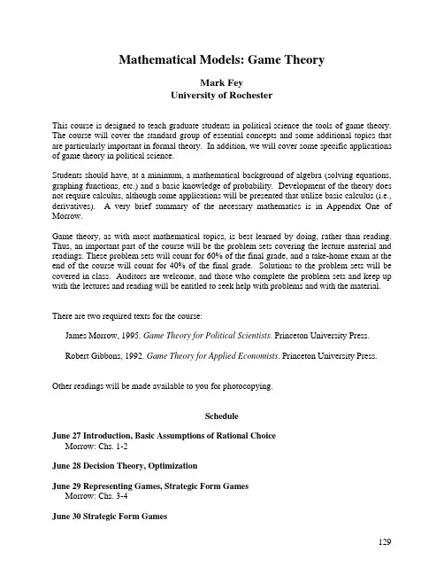
Mathematical Models: Game TheoryMark FeyUniversity of RochesterThis course is designed to teach graduate students in political science the tools of game theory. The course will cover the standard group of essential concepts and some additional topics that are particularly important in formal theory. In addition, we will cover some specific applications of game theory in political science.Students should have, at a minimum, a mathematical background of algebra (solving equations, graphing functions, etc.) and a basic knowledge of probability. Development of the theory does not require calculus, although some applications will be presented that utilize basic calculus (i.e., derivatives). A very brief summary of the necessary mathematics is in Appendix One of Morrow.Game theory, as with most mathematical topics, is best learned by doing, rather than reading. Thus, an important part of the course will be the problem sets covering the lecture material and readings. These problem sets will count for 60% of the final grade, and a take-home exam at the end of the course will count for 40% of the final grade. Solutions to the problem sets will be covered in class. Auditors are welcome, and those who complete the problem sets and keep up with the lectures and reading will be entitled to seek help with problems and with the material. There are two required texts for the course:James Morrow, 1995. Game Theory for Political Scientists. Princeton University Press.Robert Gibbons, 1992. Game Theory for Applied Economists. Princeton University Press. Other readings will be made available to you for photocopying.ScheduleJune 27Introduction, Basic Assumptions of Rational ChoiceMorrow: Chs. 1-2June 28 Decision Theory, OptimizationJune 29 Representing Games, Strategic Form GamesMorrow: Chs. 3-4June 30 Strategic Form Games129July 3 & 4 No class, but lots of fireworks!July 5 Strategic Form Games, DominanceGibbons: Sec. 1.1July 6 Nash Equilibrium, Mixed StrategiesGibbons: Sec. 1.3July 7 Zero-sum Games, ApplicationsJuly 10 Extensive Form Games, Backwards Induction Morrow: Ch. 5July 11 Subgame Perfection, Forward InductionGibbons: Ch. 2July 12 Bayesian Games, Bayesian EquilibriumMorrow: Ch. 6July 13 Bayesian EquilibriumGibbons: Ch. 3July 14 Perfect Bayesian Equilibrium and Sequential Equilibrium Morrow: Ch. 7Gibbons: Sec. 4.1July 17 Sequential EquilibriumJuly 18 Signaling GamesMorrow: Ch. 8Gibbons: Sec. 4.2July 19 Cheap Talk GamesGibbons: Sec. 4.3July 20 Repeated GamesMorrow: Ch. 9July 21 Applications, Wrap-up130。

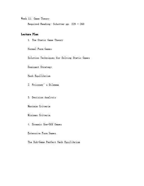
Week 11: Game TheoryRequired Reading: Schotter pp. 229 - 260Lecture Plan1. The Static Game TheoryNormal Form GamesSolution Techniques for Solving Static Games Dominant StrategyNash Equilibrium2. Prisoner’s Dilemma3. Decision AnalysisMaximim CriteriaMinimax Criteria4. Dynamic One-Off GamesExtensive Form GamesThe Sub-Game Perfect Nash Equilibrium1. The static Game TheoryStatic games: the players make their move in isolation without knowing what other players have done1.1 Normal Form GamesIn game theory there are two ways in which a game can be represented.1st) The normal form game or strategic form game2nd) The extensive form gameA normal form game is any game where we can identity the following three things:1. Players:2. The strategies available to each player.3. The Payoffs. A payoff is what a player will receive at the endof the game contingent upon the actions of all players in the game.Suppose that two people (A and B) are playing a simple game. A will write one of two words on a piece of paper, “Top” or “Bottom”. At the same time, B will independently write “left” or “right” on a piece of paper. After they do this, the papers will be examined and they will get the payoff depicted in Table 1.Table 1If A says top and B says left, then we examine the top-left corner of the matrix. In this matrix, the payoff to A(B) is the first(Second) entry in the box. For example, if A writes “top” and B writes “left” payoff of A = 1 payoff of B = 2.What is/are the equilibrium outcome(s) of this game?1.2Nash Equilibrium Approach to Solving Static GamesNash equilibrium is first defined by John Nash in 1951 based on the work of Cournot in 1893.A pair of strategy is Nash equilibrium if A's choice is optimal given B's choice, and B's choice is optimal given A's choice. When this equilibrium outcome is reached, neither individual wants to change his behaviour.Finding the Nash equilibrium for any game involves two stages.1) identify each optimal strategy in response to what the other players might do.Given B chooses left, the optimal strategy for A isGiven B chooses right, the optimal strategy for A isGiven A chooses top, the optimal strategy for B isGiven A chooses bottom, the optimal strategy for B isWe show this by underlying the payoff element for each case.2) a Nash equilibrium is identified when all players are player their optimal strategies simultaneouslyIn the case of Table 2,If A chooses top, then the best thing for B to do is to choose left since the payoff to B from choosing left is 1 and the payoff from choosing right is 0. If B chooses left, then the best thing for A to do is to choose top as A will get a payoff of 2 rather than 0.Thus if A chooses top B chooses left. If B chooses left, A chooses top. Therefore we have a Nash equilibrium: each person is making optimal choice, given the other person's choice.If the payoff matrix changes as:Table 2then what is the Nash equilibrium?Table 3If the payoffs are changed as shown in Table 32. Prisoners’ dilemm aPareto Efficiency: An allocation is Pareto efficient if goods cannot be reallocated to make someone better off without making someone else worse off.Two prisoners who were partners in a crime were being questioned in separate rooms. Each prisoner has a choice of confessing to the crime (implicating the other) or denying. If only one confesses, then he would go free and his partner will spend 6 months in prison. If both prisoners deny, then both would be in the prison for 1 month. If both confess, they would both be held for three months. The payoff matrix for this game is depicted in Table 4.Table 4The equilibrium outcome3. Decision AnalysisLet N=1 to 4 a set of possible states of nature, and let S=1 to 4be a set of strategy decided by you. Now you have to decide which strategy you have to choose given the following payoff matrix.Table 5S=YouN=OpponentIn this case you don't care the payoff of your opponent i.e. nature.3.1 The Maximin Decision Rule or Wald criterionWe look for the minimum pay-offs in each choice and then maximising the minimum pay-offLet us highlight the mimimum payoff for each strategy.3.2 The Minimax Decision Rule or Savage criterionOn this rule we need to compute the losses or regret matrix from the payoff matrix. The losses are defined as the difference between the actual payoff and what that payoff would have been had the correct strategy been chosen.Regret/Loss = Max. payoff in each column – actual payoffFor example of N=1 occurs and S=1 is chosen, the actual gain = 2 from Table 3. However, the best action given N=1 is also to choose S=1 which gives the best gain = 2. For (N=1, S=1) regret = 0.If N=1 occurs but S=2 is chosen, the actual gain = 1. However, the best action given N=1 is also to choose S=1 which gives the best gain = 2. For (N=1, S=2) regret = 2-1.Following the similar analysis, we can compute the losses for each N and S and so can compute the regret matrix.Table 6: Regret MatrixAfter computing the regret matrix, we look for the maximum regret of each strategy and then taking the minimum of these.Minimax is still very cautious but less so than the maximin.4. Dynamic one-off GamesA game can be dynamic for two reasons. First, players may be ableto observe the actions of other players before deciding upon theiroptimal response. Second, one-off game may be repeated a number of times.4.1 Extensive Form GamesDynamic games cannot be represented by payoff matrices we have touse a decision tree (extensive form) to represent a dynamic game.Start with the concept of dynamic one-off game the game can beplayed for only one time but players can condition their optimal actions on what other players have done in the past.Suppose that there are two firms (A and B) that are considering whether or not to enter a new market. If both firms enter the market,then they will make a loss of $10 mil. If only one firm enters the market, it will earn a profit of $50 mil. Suppose also that Firm B observes whether Firm A has entered the market before it decides what to do.Any extensive form game has the following four elements in common:Nodes: This is a position where the players must take a decision.The first position is called the initial node, and each node is labelled so as to identify who is making the decision.Branches: These represent the alternative choices that the person faces and so correspond to available actions.Payoff Vectors: These represent the payoffs for each player, with the payoffs listed in the order of players. When we reach a payoffvector the game ends.In period 1, Firm A makes its decisions. This is observed by Firm B which decides to enter or stay out of the market in period 2. In this extensive form game, Firm B’s decision nodes are the sub-game. This means that firm B observes Firm A’s action before making its own decision.4.2 Subgame Perfect Nash EquilibriumSubgame perfect Nash equilibrium is the predicted solution to a dynamic one-off game. From the extensive form of this game, we can observe that there are two subgames, one starting from each of Firm B’s decision nodes.How could we identify the equilibrium outcomes?In applying this principle to this dynamic game, we start with the last period first and work backward through successive nodes until we reach the beginning of the game.Start with the last period of the game first, we have two nodes. At each node, Firm B decides whether or not entering the market based on what Firm A has already done.For example, at the node of “Firm A enters”, Firm B will either make a loss of –$10mil (if it enters) or receive “0” payoff (if it stays out); these are shown by the payoff vectors (-10, -10) and (50, 0). If Firm B is rational, it will stays outThe node “Firm A enters” can be replaced by the vector (50, 0).At the second node “Firm A stays out”, Firm A h as not entered the market. Thus, Firm B will either make a profit of $50mil (if it enters) or receive “0” payoff (if it stays out); these are shown by the payoff vectors (0, 50) and (0, 0). If Firm B is rational, it will enter thus we could rule out the possibility of both firms stay outWe can now move back to the initial node. Here Firm A has to decide whether or not to enter. If Firm B is rational, it is known that the game will never reach the previously “crossed” vectors. Firm A also knows that if it enters, the game will eventually end at (A enters, B stays out) where A gets 50 and B gets 0. On the other hand, if Firm A stays out, the game will end at (A stays out, B enters) where A gets 0 and B gets 50 Firm A should enter the market at the first stage. The eventual outcome is (A enters, B stays out)How to find a subgame perfect equilibrium of a dynamic one-off game?1. Start with the last period of the game cross out the irrelevant payoff vectors.2. Replace the preceding nodes by the uncrossed payoff vectorsuntil you reach the initial node.3. The only uncrossed payoff vector(s) is the subgame perfect Nash equilibrium.。

POLS 606 (601): Game TheoryProfessor Ahmer TararSpring 2006Monday 1-3:50 p.m., 2064 Allen BuildingOffice: 2045 Allen BuildingOffice Hours: Tuesday 2-4 p.m. and by appointmentOffice Phone: 845-2628Email: ***********************.eduPurpose: Game theory is a set of mathematical tools used to study multi-player interdependent decision making (often called strategic decision making). Strategic decision-making is used in situations where the outcome depends on the actions of more than one actor, and hence each actor, in choosing his or her optimal course of action, must take into account the expected behavior of the other actors. Such situations arise in all areas of politics, from legislators considering what legislation to introduce and how to vote on it (keeping in mind how they expect other legislators to vote, and whether or not the president will veto it in the US case), to candidates for political office deciding which policy positions to choose (keeping in mind how they expect voters to vote based on their policy preferences), and nations deciding whether or not to attack other nations (keeping in mind how their own and the other side's allies will react). Because analyzing such situations can become extremely complicated, verbal reasoning can easily lead to mistakes and the use of mathematics becomes very helpful.The purpose of this course is to give students an introductory but solid exposure to the main topics in noncooperative game theory. (Game theory has two branches, cooperative and noncooperative. Cooperative game theory is used to study strategic decision-making when the actors are allowed to make binding agreements to take certain actions; noncooperative game theory is used to study situations where the actors can't, and the actors always choose their actions according to their preferences. The latter is used much more extensively than the former in political science, and in economics as well, and hence we will concentrate on it.) I anticipate that many of the students taking this course do not plan to do advanced modeling in their own research, but want to be able to understand the game-theoretic political science literature. To this end, the course will emphasize the ideas and concepts of game theory rather than the mathematical details. However, the course will also be rigorous enough that students who decided that they want to develop advanced game-theoretic models in their own research will have a firm foundation for pursuing that goal.Course Requirements: Game theory can only be learnt by solving problems. Even if you think you understand everything in lecture, you will realize that you don't once you try solving game theory problems. Therefore, there will be weekly (or semi-weekly) homework assignments that will usually be due a week after they are assigned. There will also be a midterm exam and a final exam, which may or may not be take-home exams (I will announce this later).Readings:The only required textbook is Martin J. Osborne's An Introduction to Game Theory (2004, Oxford University Press). The book is really nice for a game theory text because it is very explanatory and yet uses rigorous definitions. It also has tons of examples, including many from political science, which is rare for a game theory text.There are a number of other game theory texts that students may find useful. Game Theory for Applied Economists (by Robert Gibbons, 1992, Princeton University Press) does an excellent job of very clearly explaining the solution concepts for different types of games. I highly recommend it. A Course in Game Theory (by Osborne and Rubinstein, 1994, MIT Press) is an advanced graduate-level text that uses most of the same notation as our text. It is quite advanced and rigorous, and I highly recommend it for any student who wants to seriously pursue advanced game theory. (I might occasionally prove some results from this text in class.) The same goes for Game Theory (by Fudenberg and Tirole, 1991, MIT Press), another very advanced and especially comprehensive text. Finally, for students who want a very basic yet engaging introduction to game theory, there is Thinking Strategically (by Dixit and Nalebuff, 1991, Norton).Students With Disabilities Policy:The Americans with Disabilities Act (ADA) is a federal anti-discrimination statute that provides comprehensive civil rights protection for persons with disabilities. Among other things, this legislation requires that all students with disabilities be guaranteed a learning environment that provides for reasonable accommodation of their disabilities. If you believe you have a disability requiring an accommodation, please contact the Department of Student Life, Services for Students with Disabilities in Room 126 of the Koldus Building, or call 845-1637.Course Materials/Copyright Statement:The handouts used in this course are copyrighted. By "handouts," I mean all materials generated for this class, which include but are not limited to syllabi, quizzes, exams, lab problems, in-class materials review sheets, and additional problem sets. Because these are copyrighted, you do not have the right to copy the handouts, unless I expressly grant permission.Plagiarism Statement:As commonly defined, plagiarism consists of passing off as one's own the ideas, words, writings, etc., which belong to another. In accordance with the definition, you are committing plagiarism if you copy the work of another person and turn it in as your own, even if you should have the permission of the person. Plagiarism is one of the worst academic sins, for the plagiarist destroys the trust among colleagues without which research cannot be safely communicated. If you have any questions regarding plagiarism,please consult the latest issue of the Texas A&M University Student Rules, under the section "Scholastic Dishonesty."Tentative Course Schedule:The following is an outline of the order in which we will cover topics. It is subject to change during the course of the semester. We may or may not get to some of the special topics.Topic 1: Mathematical Preliminaries, and Introduction to Game Theory and the Theory of Rational Choice: Ch. 17, 1Topic 2: Strategic Form Games: Nash Equilibrium: Ch. 2, 3 (parts)Topic 3: Strategic Form Games: Mixed Strategy Equilibrium, Strictly Competitive Games, Rationalizability: Ch. 4, 11, 12Topic 4: Bayesian Games: Ch. 9Topic 5: Extensive Form Games with Perfect Information: Ch. 5, 6 (parts), 7 (parts) Topic 6: Extensive Form Games with Imperfect Information: Ch. 10Topic 7: Repeated Games: Ch. 14, 15Special Topic 1: Evolutionary Equilibrium: Ch. 13Special Topic 2: Bargaining: Ch. 16 and Baron and Ferejohn 1989 APSR "Bargaining in Legislatures" articleSpecial Topic 3: Social Choice TheorySpecial Topic 4: Coalitional Games and the Core: Ch. 8。

Lecture5:Subgame Perfect EquilibriumNovember1,2006Osborne:ch7How do we analyze extensive form games where there are simultaneous moves? Example:Stage1.Player1chooses between f IN,OUT gIf OUT,game ends,player1gets2and player2gets3If IN,the proceed to stage2,where both players play a simultaneous move game, one-sided prisoners'dilemmaL RT4,30,0B5,01,1In stage2we cannot use backwards induction.But we know how to solve stage2:a Nash equilibrium must be played.Unique NE is stage2,(B;R)Since IN yields payo of1to player1,optimal to choose OUT in stage1.What if there is not a unique prediction in stage2? Eg.stage2game is Hawk-dove game.h dH-1,-14,1D1,42,2In stage2,a Nash equilibrium must be played.Two pure strategy Nash equilibria,(H;d)and(D;h):a)Suppose that(H;d)will be played)payo s will be(4,1)in stage2So in stage1,player1must choose INb)Suppose that(d;H)will be played)payo s will be(1,4)in stage2So in stage1,player1must choose OUT. Two pure strategy subgame perfect equilibria.i)Player1plays IN(in stage1)and H in stage2;player2plays d in stage2. (IN;H;d)ii)Player1plays OUT(in stage1)and d in stage2;player2plays H in stage2. (OUT;d;H)Extensive game with perfect information and simultaneous moves1.Set of players N2.set of nodes X or histories3.E X is a terminal node or history.4.Every player has a payo associated with every terminal node.4.At any history h2X E;a subset of players has to choose an action.(player function)at this node,every player knows what actions have been taken by other players before this.5.at any h where player i has to choose an action A i(h)is the set of available actions.6.Any non terminal node h and the action pro le chosen at h lead to another node h02XA(pure)strategy for a player in an extensive game of perfect information is a plan that speci es an action at each decision node that belongs to her.X i:set of decision nodes where player i must chooseNow more than one player may choose at each decision node.A(x)set of actions available at decision mode xA pure strategy for player i is a function s i:!A(x)satisfying s i(x)2A(x)S i is the set of pure strategies for iIn example,S i=f OUT&T,OUT&B,IN&T,IN&B gSpeci es actions even at nodes that are ruled out by own strategy.If we x a pure strategy for each player,this is a pure strategy pro le s= (s1;s2;:::;s n)This pro le fully determines what happens in the game.If there is no randomness(chance moves),then there is determinate terminal node that results.(if there are chance moves,then s determines a probability distribution over E)So s gives rise to a payo for each player.(S i;u i)i2I is the strategic form ofWe can therefore analyze by analysing its strategic form We can solve for the Nash equilibria of the strategic formA subgame of a extensive game is the game starting from some node x;where one or more players move simultaneously.Subgame Perfect Nash Equilibrium:a pro le of strategies s=(s1;s2;:::;s n) is a subgame perfect Nash equilibrium if a Nash equilibrium is played in every subgame.Example1:(OUT&B,L)is a subgame perfect Nash equilibriumExample2:(IN;H;d)is one SPE(OUT;d;H)is another SPECommittee Decision making(ch7,Osborne) Example:3member committee f A;B;C g3alternatives X=f x;y;z gA B Cx y zy z xz x yStrict preference orderingsVoting system:binary agendastage1:members simultaneously vote whether to adopt x or not If x is chosen,end of story,if notstage2:vote between y and z:majority vote at each stage.members vote strategically{sophisticated votinganticipate the e ects of their choices in futureAnalysis:Stage2:A&B strictly prefer y to zOne Nash equilibrium at this stage where A&b vote for y;y wins (Another Nash equilibrium where all voters vote for same alternative(say z) since no one can make a di erence(with two others voting for z;this is a NE Nash equilibrium involves weakly dominated choice{not reasonable.So y is chosen in stage2In stage1,choice between x and y.A&C strictly prefer x to ytherefore x will be chosen in the subgame perfect equilibrium where voters do not use dominated choices.General model of voting in binary agendasn alternative.odd number of committee members with strict preference orderings(no indi er-ence)majority vote in each stageBinary agenda:sequential procedureadopt x1or not;if not,adopt x2or not;&so on..di erent binary agenda for di erent ordering of votes(e.g.x n;x n 1;:::;x1)What will be the result of sophisticated voting in binary agendas? x beats y if a majority of the committee prefer x to yIf x beats every other alternative,x is a Condorcet winnerA B Cx y yy z xz x zy is a Condorcet winnerCondorcet winner y need not Pareto dominate xProposition:If a Condorcet winner x exists,then x is the undominated subgame perfect equilibrium outcome of any binary agendaProof:By backwards induction,we can determine alternative that will result at any node.At the node h where x can be adopted:Let y be the alternative that will be chosen if x is not chosen.A majority prefers x to y;so x will be adopted at hBy backwards induction,every preceding alternative will be rejected so that we get to hsince x beats every other alternative.What happens if there is no Condorcet winner?x indirectly beats y if eithera)x beats y;orb)there is a sequence of alternatives u1;u2;:::;u k such thatx beats u1&u1beats u2&::::u k 1beats u k&u k beats y:A set of alternatives S X such that every x2S indirectly beats every other alternative in y is a top cycle set.Proposition:If x is the winner of some binary agenda,then x must belong to the top cycle set.Proposition:If x belongs to the top cycle set,then there is some binary agenda such that x wins.。

GAME THEORYThomas S.Ferguson Part II.Two-Person Zero-Sum Games1.The Strategic Form of a Game.1.1Strategic Form.1.2Example:Odd or Even.1.3Pure Strategies and Mixed Strategies.1.4The Minimax Theorem.1.5Exercises.2.Matrix Games.Domination.2.1Saddle Points.2.2Solution of All2by2Matrix Games.2.3Removing Dominated Strategies.2.4Solving2×n and m×2Games.2.5Latin Square Games.2.6Exercises.3.The Principle of Indifference.3.1The Equilibrium Theorem.3.2Nonsingular Game Matrices.3.3Diagonal Games.3.4Triangular Games.3.5Symmetric Games.3.6Invariance.3.7Exercises.4.Solving Finite Games.4.1Best Responses.4.2Upper and Lower Values of a Game.4.3Invariance Under Change of Location and Scale.4.4Reduction to a Linear Programming Problem.4.5Description of the Pivot Method for Solving Games.4.6A Numerical Example.4.7Exercises.5.The Extensive Form of a Game.5.1The Game Tree.5.2Basic Endgame in Poker.5.3The Kuhn Tree.5.4The Representation of a Strategic Form Game in Extensive Form.5.5Reduction of a Game in Extensive Form to Strategic Form.5.6Example.5.7Games of Perfect Information.5.8Behavioral Strategies.5.9Exercises.6.Recursive and Stochastic Games.6.1Matrix Games with Games as Components.6.2Multistage Games.6.3Recursive Games. -Optimal Strategies.6.4Stochastic Movement Among Games.6.5Stochastic Games.6.6Approximating the Solution.6.7Exercises.7.Continuous Poker Models.7.1La Relance.7.2The von Neumann Model.7.3Other Models.7.4Exercises.References.Part II.Two-Person Zero-Sum Games1.The Strategic Form of a Game.The individual most closely associated with the creation of the theory of games is John von Neumann,one of the greatest mathematicians of this century.Although others preceded him in formulating a theory of games-notably´Emile Borel-it was von Neumann who published in1928the paper that laid the foundation for the theory of two-person zero-sum games.Von Neumann’s work culminated in a fundamental book on game theory written in collaboration with Oskar Morgenstern entitled Theory of Games and Economic Behavior,1944.Other more current books on the theory of games may be found in the text book,Game Theory by Guillermo Owen,2nd edition,Academic Press,1982,and the expository book,Game Theory and Strategy by Philip D.Straffin,published by the Mathematical Association of America,1993.The theory of von Neumann and Morgenstern is most complete for the class of games called two-person zero-sum games,i.e.games with only two players in which one player wins what the other player loses.In Part II,we restrict attention to such games.We will refer to the players as Player I and Player II.1.1Strategic Form.The simplest mathematical description of a game is the strate-gic form,mentioned in the introduction.For a two-person zero-sum game,the payofffunction of Player II is the negative of the payoffof Player I,so we may restrict attention to the single payofffunction of Player I,which we call here L.Definition1.The strategic form,or normal form,of a two-person zero-sum game is given by a triplet(X,Y,A),where(1)X is a nonempty set,the set of strategies of Player I(2)Y is a nonempty set,the set of strategies of Player II(3)A is a real-valued function defined on X×Y.(Thus,A(x,y)is a real number for every x∈X and every y∈Y.)The interpretation is as follows.Simultaneously,Player I chooses x∈X and Player II chooses y∈Y,each unaware of the choice of the other.Then their choices are made known and I wins the amount A(x,y)from II.Depending on the monetary unit involved, A(x,y)will be cents,dollars,pesos,beads,etc.If A is negative,I pays the absolute value of this amount to II.Thus,A(x,y)represents the winnings of I and the losses of II.This is a very simple definition of a game;yet it is broad enough to encompass the finite combinatorial games and games such as tic-tac-toe and chess.This is done by being sufficiently broadminded about the definition of a strategy.A strategy for a game of chess,for example,is a complete description of how to play the game,of what move to make in every possible situation that could occur.It is rather time-consuming to write down even one strategy,good or bad,for the game of chess.However,several different programs for instructing a machine to play chess well have been written.Each program constitutes one strategy.The program Deep Blue,that beat then world chess champion Gary Kasparov in a match in1997,represents one strategy.The set of all such strategies for Player I is denoted by X.Naturally,in the game of chess it is physically impossible to describe all possible strategies since there are too many;in fact,there are more strategies than there are atoms in the known universe.On the other hand,the number of games of tic-tac-toe is rather small,so that it is possible to study all strategies andfind an optimal strategy for each ter,when we study the extensive form of a game,we will see that many other types of games may be modeled and described in strategic form.To illustrate the notions involved in games,let us consider the simplest non-trivial case when both X and Y consist of two elements.As an example,take the game called Odd-or-Even.1.2Example:Odd or Even.Players I and II simultaneously call out one of the numbers one or two.Player I’s name is Odd;he wins if the sum of the numbers if odd. Player II’s name is Even;she wins if the sum of the numbers is even.The amount paid to the winner by the loser is always the sum of the numbers in dollars.To put this game in strategic form we must specify X,Y and A.Here we may choose X={1,2},Y={1,2}, and A as given in the following table.II(even)yI(odd)x12 1−2+3 2+3−4A(x,y)=I’s winnings=II’s losses.It turns out that one of the players has a distinct advantage in this game.Can you tell which one it is?Let us analyze this game from Player I’s point of view.Suppose he calls‘one’3/5ths of the time and‘two’2/5ths of the time at random.In this case,1.If II calls‘one’,I loses2dollars3/5ths of the time and wins3dollars2/5ths of the time;on the average,he wins−2(3/5)+3(2/5)=0(he breaks even in the long run).2.If II call‘two’,I wins3dollars3/5ths of the time and loses4dollars2/5ths of the time; on the average he wins3(3/5)−4(2/5)=1/5.That is,if I mixes his choices in the given way,the game is even every time II calls ‘one’,but I wins20/c on the average every time II calls‘two’.By employing this simple strategy,I is assured of at least breaking even on the average no matter what II does.Can Player Ifix it so that he wins a positive amount no matter what II calls?Let p denote the proportion of times that Player I calls‘one’.Let us try to choose p so that Player I wins the same amount on the average whether II calls‘one’or‘two’.Then since I’s average winnings when II calls‘one’is−2p+3(1−p),and his average winnings when II calls‘two’is3p−4(1−p)Player I should choose p so that−2p+3(1−p)=3p−4(1−p)3−5p=7p−412p=7p=7/12.Hence,I should call‘one’with probability7/12,and‘two’with probability5/12.On theaverage,I wins−2(7/12)+3(5/12)=1/12,or813cents every time he plays the game,nomatter what II does.Such a strategy that produces the same average winnings no matter what the opponent does is called an equalizing strategy.Therefore,the game is clearly in I’s favor.Can he do better than813cents per gameon the average?The answer is:Not if II plays properly.In fact,II could use the same procedure:call‘one’with probability7/12call‘two’with probability5/12.If I calls‘one’,II’s average loss is−2(7/12)+3(5/12)=1/12.If I calls‘two’,II’s average loss is3(7/12)−4(5/12)=1/12.Hence,I has a procedure that guarantees him at least1/12on the average,and II has a procedure that keeps her average loss to at most1/12.1/12is called the value of the game,and the procedure each uses to insure this return is called an optimal strategy or a minimax strategy.If instead of playing the game,the players agree to call in an arbitrator to settle thisconflict,it seems reasonable that the arbitrator should require II to pay813cents to I.ForI could argue that he should receive at least813cents since his optimal strategy guaranteeshim that much on the average no matter what II does.On the other hand II could arguethat he should not have to pay more than813cents since she has a strategy that keeps heraverage loss to at most that amount no matter what I does.1.3Pure Strategies and Mixed Strategies.It is useful to make a distinction between a pure strategy and a mixed strategy.We refer to elements of X or Y as pure strategies.The more complex entity that chooses among the pure strategies at random in various proportions is called a mixed strategy.Thus,I’s optimal strategy in the game of Odd-or-Even is a mixed strategy;it mixes the pure strategies one and two with probabilities 7/12and5/12respectively.Of course every pure strategy,x∈X,can be considered as the mixed strategy that chooses the pure strategy x with probability1.In our analysis,we made a rather subtle assumption.We assumed that when a player uses a mixed strategy,he is only interested in his average return.He does not care about hismaximum possible winnings or losses—only the average.This is actually a rather drastic assumption.We are evidently assuming that a player is indifferent between receiving5 million dollars outright,and receiving10million dollars with probability1/2and nothing with probability1/2.I think nearly everyone would prefer the$5,000,000outright.This is because the utility of having10megabucks is not twice the utility of having5megabucks.The main justification for this assumption comes from utility theory and is treated in Appendix1.The basic premise of utility theory is that one should evaluate a payoffby its utility to the player rather than on its numerical monetary value.Generally a player’s utility of money will not be linear in the amount.The main theorem of utility theory states that under certain reasonable assumptions,a player’s preferences among outcomes are consistent with the existence of a utility function and the player judges an outcome only on the basis of the average utility of the outcome.However,utilizing utility theory to justify the above assumption raises a new difficulty. Namely,the two players may have different utility functions.The same outcome may be perceived in quite different ways.This means that the game is no longer zero-sum.We need an assumption that says the utility functions of two players are the same(up to change of location and scale).This is a rather strong assumption,but for moderate to small monetary amounts,we believe it is a reasonable one.A mixed strategy may be implemented with the aid of a suitable outside random mechanism,such as tossing a coin,rolling dice,drawing a number out of a hat and so on.The seconds indicator of a watch provides a simple personal method of randomization provided it is not used too frequently.For example,Player I of Odd-or-Even wants an outside random event with probability7/12to implement his optimal strategy.Since 7/12=35/60,he could take a quick glance at his watch;if the seconds indicator showed a number between0and35,he would call‘one’,while if it were between35and60,he would call‘two’.1.4The Minimax Theorem.A two-person zero-sum game(X,Y,A)is said to be afinite game if both strategy sets X and Y arefinite sets.The fundamental theorem of game theory due to von Neumann states that the situation encountered in the game of Odd-or-Even holds for allfinite two-person zero-sum games.Specifically,The Minimax Theorem.For everyfinite two-person zero-sum game,(1)there is a number V,called the value of the game,(2)there is a mixed strategy for Player I such that I’s average gain is at least V no matter what II does,and(3)there is a mixed strategy for Player II such that II’s average loss is at most V no matter what I does.This is one form of the minimax theorem to be stated more precisely and discussed in greater depth later.If V is zero we say the game is fair.If V is positive,we say the game favors Player I,while if V is negative,we say the game favors Player II.1.5Exercises.1.Consider the game of Odd-or-Even with the sole change that the loser pays the winner the product,rather than the sum,of the numbers chosen(who wins still depends on the sum).Find the table for the payofffunction A,and analyze the game tofind the value and optimal strategies of the players.Is the game fair?2.Player I holds a black Ace and a red8.Player II holds a red2and a black7.The players simultaneously choose a card to play.If the chosen cards are of the same color, Player I wins.Player II wins if the cards are of different colors.The amount won is a number of dollars equal to the number on the winner’s card(Ace counts as1.)Set up the payofffunction,find the value of the game and the optimal mixed strategies of the players.3.Sherlock Holmes boards the train from London to Dover in an effort to reach the continent and so escape from Professor Moriarty.Moriarty can take an express train and catch Holmes at Dover.However,there is an intermediate station at Canterbury at which Holmes may detrain to avoid such a disaster.But of course,Moriarty is aware of this too and may himself stop instead at Canterbury.Von Neumann and Morgenstern(loc.cit.) estimate the value to Moriarty of these four possibilities to be given in the following matrix (in some unspecified units).HolmesMoriartyCanterbury Dover Canterbury100−50 Dover0100What are the optimal strategies for Holmes and Moriarty,and what is the value?(His-torically,as related by Dr.Watson in“The Final Problem”in Arthur Conan Doyle’s The Memoires of Sherlock Holmes,Holmes detrained at Canterbury and Moriarty went on to Dover.)4.The entertaining book The Compleat Strategyst by John Williams contains many simple examples and informative discussion of strategic form games.Here is one of his problems.“I know a good game,”says Alex.“We pointfingers at each other;either onefinger or twofingers.If we match with onefinger,you buy me one Daiquiri,If we match with twofingers,you buy me two Daiquiris.If we don’t match I letyou offwith a payment of a dime.It’ll help pass the time.”Olaf appears quite unmoved.“That sounds like a very dull game—at least in its early stages.”His eyes glaze on the ceiling for a moment and his lipsflutterbriefly;he returns to the conversation with:“Now if you’d care to pay me42cents before each game,as a partial compensation for all those55-cent drinks I’llhave to buy you,then I’d be happy to pass the time with you.Olaf could see that the game was inherently unfair to him so he insisted on a side payment as compensation.Does this side payment make the game fair?What are the optimal strategies and the value of the game?2.Matrix Games —DominationA finite two-person zero-sum game in strategic form,(X,Y,A ),is sometimes called a matrix game because the payofffunction A can be represented by a matrix.If X ={x 1,...,x m }and Y ={y 1,...,y n },then by the game matrix or payoffmatrix we mean the matrix A =⎛⎝a 11···a 1n ......a m 1···a mn⎞⎠where a ij =A (x i ,y j ),In this form,Player I chooses a row,Player II chooses a column,and II pays I the entry in the chosen row and column.Note that the entries of the matrix are the winnings of the row chooser and losses of the column chooser.A mixed strategy for Player I may be represented by an m -tuple,p =(p 1,p 2,...,p m )of probabilities that add to 1.If I uses the mixed strategy p =(p 1,p 2,...,p m )and II chooses column j ,then the (average)payoffto I is m i =1p i a ij .Similarly,a mixed strategy for Player II is an n -tuple q =(q 1,q 2,...,q n ).If II uses q and I uses row i the payoffto I is n j =1a ij q j .More generally,if I uses the mixed strategy p and II uses the mixed strategy q ,the (average)payoffto I is p T Aq = m i =1 n j =1p i a ij q j .Note that the pure strategy for Player I of choosing row i may be represented as the mixed strategy e i ,the unit vector with a 1in the i th position and 0’s elsewhere.Similarly,the pure strategy for II of choosing the j th column may be represented by e j .In the following,we shall be attempting to ‘solve’games.This means finding the value,and at least one optimal strategy for each player.Occasionally,we shall be interested in finding all optimal strategies for a player.2.1Saddle points.Occasionally it is easy to solve the game.If some entry a ij of the matrix A has the property that(1)a ij is the minimum of the i th row,and(2)a ij is the maximum of the j th column,then we say a ij is a saddle point.If a ij is a saddle point,then Player I can then win at least a ij by choosing row i ,and Player II can keep her loss to at most a ij by choosing column j .Hence a ij is the value of the game.Example 1.A =⎛⎝41−3325016⎞⎠The central entry,2,is a saddle point,since it is a minimum of its row and maximum of its column.Thus it is optimal for I to choose the second row,and for II to choose the second column.The value of the game is 2,and (0,1,0)is an optimal mixed strategy for both players.For large m ×n matrices it is tedious to check each entry of the matrix to see if it has the saddle point property.It is easier to compute the minimum of each row and the maximum of each column to see if there is a match.Here is an example of the method.row min A =⎛⎜⎝3210012010213122⎞⎟⎠0001col max 3222row min B =⎛⎜⎝3110012010213122⎞⎟⎠0001col max 3122In matrix A ,no row minimum is equal to any column maximum,so there is no saddle point.However,if the 2in position a 12were changed to a 1,then we have matrix B .Here,the minimum of the fourth row is equal to the maximum of the second column;so b 42is a saddle point.2.2Solution of All 2by 2Matrix Games.Consider the general 2×2game matrix A = a b d c.To solve this game (i.e.to find the value and at least one optimal strategy for each player)we proceed as follows.1.Test for a saddle point.2.If there is no saddle point,solve by finding equalizing strategies.We now prove the method of finding equalizing strategies of Section 1.2works when-ever there is no saddle point by deriving the value and the optimal strategies.Assume there is no saddle point.If a ≥b ,then b <c ,as otherwise b is a saddle point.Since b <c ,we must have c >d ,as otherwise c is a saddle point.Continuing thus,we see that d <a and a >b .In other words,if a ≥b ,then a >b <c >d <a .By symmetry,if a ≤b ,then a <b >c <d >a .This shows thatIf there is no saddle point,then either a >b ,b <c ,c >d and d <a ,or a <b ,b >c ,c <d and d >a .In equations (1),(2)and (3)below,we develop formulas for the optimal strategies and value of the general 2×2game.If I chooses the first row with probability p (es the mixed strategy (p,1−p )),we equate his average return when II uses columns 1and 2.ap +d (1−p )=bp +c (1−p ).Solving for p ,we findp =c −d (a −b )+(c −d ).(1)Since there is no saddle point,(a−b)and(c−d)are either both positive or both negative; hence,0<p<1.Player I’s average return using this strategy isv=ap+d(1−p)=ac−bda−b+c−d.If II chooses thefirst column with probability q(es the strategy(q,1−q)),we equate his average losses when I uses rows1and2.aq+b(1−q)=dq+c(1−q)Hence,q=c−ba−b+c−d.(2)Again,since there is no saddle point,0<q<1.Player II’s average loss using this strategyisaq+b(1−q)=ac−bda−b+c−d=v,(3)the same value achievable by I.This shows that the game has a value,and that the players have optimal strategies.(something the minimax theorem says holds for allfinite games). Example2.A=−233−4p=−4−3−2−3−4−3=7/12q=samev=8−9−2−3−4−3=1/12Example3.A=0−1012p=2−10+10+2−1=1/11q=2+100+10+2−1=12/11.But q must be between zero and one.What happened?The trouble is we“forgot to test this matrix for a saddle point,so of course it has one”.(J.D.Williams The Compleat Strategyst Revised Edition,1966,McGraw-Hill,page56.)The lower left corner is a saddle point.So p=0and q=1are optimal strategies,and the value is v=1.2.3Removing Dominated Strategies.Sometimes,large matrix games may be reduced in size(hopefully to the2×2case)by deleting rows and columns that are obviously bad for the player who uses them.Definition.We say the i th row of a matrix A=(a ij)dominates the k th row if a ij≥a kj for all j.We say the i th row of A strictly dominates the k th row if a ij>a kj for all j.Similarly,the j th column of A dominates(strictly dominates)the k th column if a ij≤a ik(resp.a ij<a ik)for all i.Anything Player I can achieve using a dominated row can be achieved at least as well using the row that dominates it.Hence dominated rows may be deleted from the matrix.A similar argument shows that dominated columns may be removed.To be more precise,removal of a dominated row or column does not change the value of a game .However,there may exist an optimal strategy that uses a dominated row or column (see Exercise 9).If so,removal of that row or column will also remove the use of that optimal strategy (although there will still be at least one optimal strategy left).However,in the case of removal of a strictly dominated row or column,the set of optimal strategies does not change.We may iterate this procedure and successively remove several rows and columns.As an example,consider the matrix,A .The last column is dominated by the middle column.Deleting the last column we obtain:A =⎛⎝204123412⎞⎠Now the top row is dominated by the bottomrow.(Note this is not the case in the original matrix).Deleting the top row we obtain:⎛⎝201241⎞⎠This 2×2matrix does not have a saddle point,so p =3/4,q =1/4and v =7/4.I’s optimal strategy in the original game is(0,3/4,1/4);II’s is (1/4,3/4,0).1241 A row (column)may also be removed if it is dominated by a probability combination of other rows (columns).If for some 0<p <1,pa i 1j +(1−p )a i 2j ≥a kj for all j ,then the k th row is dominated by the mixed strategy that chooses row i 1with probability p and row i 2with probability 1−p .Player I can do at least as well using this mixed strategy instead of choosing row k .(In addition,any mixed strategy choosing row k with probability p k may be replaced by the one in which k ’s probability is split between i 1and i 2.That is,i 1’s probability is increased by pp k and i 2’s probability is increased by (1−p )p k .)A similar argument may be used for columns.Consider the matrix A =⎛⎝046574963⎞⎠.The middle column is dominated by the outside columns taken with probability 1/2each.With the central column deleted,the middle row is dominated by the combination of the top row with probability 1/3and the bottom row with probability 2/3.The reducedmatrix, 0693,is easily solved.The value is V =54/12=9/2.Of course,mixtures of more than two rows (columns)may be used to dominate and remove other rows (columns).For example,the mixture of columns one two and threewith probabilities 1/3each in matrix B =⎛⎝135340223735⎞⎠dominates the last column,and so the last column may be removed.Not all games may be reduced by dominance.In fact,even if the matrix has a saddle point,there may not be any dominated rows or columns.The 3×3game with a saddle point found in Example 1demonstrates this.2.4Solving 2×n and m ×2games.Games with matrices of size 2×n or m ×2may be solved with the aid of a graphical interpretation.Take the following example.p 1−p 23154160Suppose Player I chooses the first row with probability p and the second row with proba-bility 1−p .If II chooses Column 1,I’s average payoffis 2p +4(1−p ).Similarly,choices of Columns 2,3and 4result in average payoffs of 3p +(1−p ),p +6(1−p ),and 5p respectively.We graph these four linear functions of p for 0≤p ≤1.For a fixed value of p ,Player I can be sure that his average winnings is at least the minimum of these four functions evaluated at p .This is known as the lower envelope of these functions.Since I wants to maximize his guaranteed average winnings,he wants to find p that achieves the maximum of this lower envelope.According to the drawing,this should occur at the intersection of the lines for Columns 2and 3.This essentially,involves solving the game in which II is restrictedto Columns 2and 3.The value of the game 3116is v =17/7,I’s optimal strategy is (5/7,2/7),and II’s optimal strategy is (5/7,2/7).Subject to the accuracy of the drawing,we conclude therefore that in the original game I’s optimal strategy is (5/7,2/7),II’s is (0,5/7,2/7,0)and the value is 17/7.Fig 2.10123456col.3col.1col.2col.4015/7pThe accuracy of the drawing may be checked:Given any guess at a solution to a game,there is a sure-fire test to see if the guess is correct ,as follows.If I uses the strategy (5/7,2/7),his average payoffif II uses Columns 1,2,3and 4,is 18/7,17/7,17/7,and 25/7respectively.Thus his average payoffis at least17/7no matter what II does.Similarly, if II uses(0,5/7,2/7,0),her average loss is(at most)17/7.Thus,17/7is the value,and these strategies are optimal.We note that the line for Column1plays no role in the lower envelope(that is,the lower envelope would be unchanged if the line for Column1were removed from the graph). This is a test for domination.Column1is,in fact,dominated by Columns2and3taken with probability1/2each.The line for Column4does appear in the lower envelope,and hence Column4cannot be dominated.As an example of a m×2game,consider the matrix associated with Figure2.2.If q is the probability that II chooses Column1,then II’s average loss for I’s three possible choices of rows is given in the accompanying graph.Here,Player II looks at the largest of her average losses for a given q.This is the upper envelope of the function.II wants tofind q that minimizes this upper envelope.From the graph,we see that any value of q between1/4and1/3inclusive achieves this minimum.The value of the game is4,and I has an optimal pure strategy:row2.Fig2.2⎛⎝q1−q154462⎞⎠123456row1row2row3011/41/2qThese techniques work just as well for2×∞and∞×2games.2.5Latin Square Games.A Latin square is an n×n array of n different letters such that each letter occurs once and only once in each row and each column.The5×5 array at the right is an example.If in a Latin square each letter is assigned a numerical value,the resulting matrix is the matrix of a Latin square game.Such games have simple solutions.The value is the average of the numbers in a row,and the strategy that chooses each pure strategy with equal probability1/n is optimal for both players.The reason is not very deep.The conditions for optimality are satisfied.⎛⎜⎜⎜⎝a b c d eb e acd c a de b d c e b ae d b a c ⎞⎟⎟⎟⎠a =1,b =2,c =d =3,e =6⎛⎜⎜⎜⎝1233626133313623362163213⎞⎟⎟⎟⎠In the example above,the value is V =(1+2+3+3+6)/5=3,and the mixed strategy p =q =(1/5,1/5,1/5,1/5,1/5)is optimal for both players.The game of matching pennies is a Latin square game.Its value is zero and (1/2,1/2)is optimal for both players.2.6Exercises.1.Solve the game with matrix−1−3−22 ,that is find the value and an optimal (mixed)strategy for both players.2.Solve the game with matrix 02t 1for an arbitrary real number t .(Don’t forget to check for a saddle point!)Draw the graph of v (t ),the value of the game,as a function of t ,for −∞<t <∞.3.Show that if a game with m ×n matrix has two saddle points,then they have equal values.4.Reduce by dominance to 2×2games and solve.(a)⎛⎜⎝5410432−10−1431−212⎞⎟⎠(b)⎛⎝1007126476335⎞⎠.5.(a)Solve the game with matrix 3240−21−45 .(b)Reduce by dominance to a 3×2matrix game and solve:⎛⎝08584612−43⎞⎠.6.Players I and II choose integers i and j respectively from the set {1,2,...,n }for some n ≥2.Player I wins 1if |i −j |=1.Otherwise there is no payoff.If n =7,for example,the game matrix is⎛⎜⎜⎜⎜⎜⎜⎜⎝0100000101000001010000010100000101000001010000010⎞⎟⎟⎟⎟⎟⎟⎟⎠。