sdarticle

英文作文articleTitle: The Impact of Technology on Education。

In today's rapidly evolving world, technology plays an increasingly significant role in every aspect of our lives, including education. The integration of technology into education has brought about both positive and negative impacts, shaping the way students learn and educators teach. This article explores the various ways in which technology influences education and discusses its implications for the future.First and foremost, technology has revolutionized the way information is accessed and disseminated. With the internet and digital devices, students now have access to a vast amount of information at their fingertips. They can easily conduct research, explore diverse perspectives, and engage with multimedia resources to enhance their learning experience. This accessibility to information has democratized education, breaking down barriers to learningand empowering students from all backgrounds to pursue knowledge.Moreover, technology has transformed the traditional classroom environment. Interactive whiteboards, educational apps, and online platforms have become commonplace, providing educators with tools to create dynamic and engaging lessons. These digital resources cater todifferent learning styles and allow for personalized instruction, enabling students to learn at their own pace and according to their individual needs. Additionally, technology facilitates collaboration among students through online forums, video conferencing, and shared documents, fostering a sense of community and enhancing communication skills.Furthermore, technology has opened up new avenues for creativity and innovation in education. Students can now utilize multimedia tools to express their ideas, create multimedia presentations, and develop digital projects. Virtual reality (VR) and augmented reality (AR) technologies offer immersive learning experiences, allowingstudents to explore virtual environments and simulate real-world scenarios. These innovative approaches not only make learning more engaging but also cultivate critical thinking, problem-solving, and digital literacy skills essential for success in the 21st century.However, despite its numerous benefits, the widespread use of technology in education also poses challenges and concerns. One major issue is the digital divide, whichrefers to the gap between those who have access to technology and those who do not. Socioeconomic disparities and inadequate infrastructure can hinder access to digital devices and high-speed internet, depriving certain students of the opportunities afforded by technology. Bridging this divide requires concerted efforts from policymakers, educators, and technology providers to ensure equitable access to technology for all students.Additionally, the overreliance on technology in education raises concerns about its potential drawbacks. Excessive screen time and digital distractions can impede students' focus and concentration, leading to decreasedacademic performance and impaired social skills. Moreover, the proliferation of online resources raises questions about the quality and credibility of information available to students. Educators must teach students how tocritically evaluate sources and discern fact from fiction in an age of information overload.In conclusion, technology has undoubtedly reshaped the landscape of education, offering unprecedentedopportunities for learning and innovation. From enhancing access to information to fostering collaboration and creativity, technology has the potential to revolutionize education for the better. However, realizing this potential requires addressing challenges such as the digital divide and mitigating the risks associated with overreliance on technology. By harnessing the power of technology responsibly, educators can empower students to thrive in a digital age and prepare them for the challenges of the future.。

sci种的article形式
SCI（Science Citation Index）是国际上具有较高学术影响力的学术期刊文献数据库。

SCI收录的文章形式包括以下几种：
1. 研究论文（research articles）：这是SCI期刊中最常见的文章形式，主要是研究者对某一具体问题进行系统研究和实验，并通过定量数据、分析和讨论得出结论。

2. 评论文章（review articles）：这类文章是作者对某一特定领域进行综述、总结和分析，旨在总结现有研究成果、提出未来研究的方向与问题，并得出结论或展望。

评论文章一般由领域内权威的研究者或专家撰写。

3. 短篇通信（short communications）：这类文章主要是对某一关键问题的初步研究结果进行通报与交流，一般篇幅较短，主要内容集中在研究的原始数据、实验方法和初步结论上。

4. 编者按（editorial）：这是SCI期刊中的一种文章形式，由期刊编辑或编委会成员撰写，主要用于介绍、评述和评论该期刊上发表的一些关键文章、研究领域现状，或对某一相关学术问题进行辨析与讨论。

5. 专论（perspective）：这类文章主要是就某一重要、前沿的学术问题或新兴研究领域进行专门评论与分析，一般由学术界的知名学者、专家所撰写。

以上是SCI期刊中常见的文章形式，每种形式的文章都有其特定的格式和撰写要求，以确保科学研究的严谨性和可信度。

article简单造句带翻译Title: The Benefits of Regular Exercise for Mental Health。

Regular exercise has numerous benefits for physical health, but it is also an effective way to improve mental health. Research has shown that exercise can help reduce symptoms of anxiety and depression, improve mood, and enhance cognitive function. In this article, we will explore the various ways in which regular exercise can benefit mental health.Firstly, exercise has been shown to reduce symptoms of anxiety and depression. Exercise releases endorphins, which are chemicals in the brain that act as natural painkillers and mood elevators. These endorphins can help reduce feelings of anxiety and depression, and improve overall mood. In addition, exercise can also help reduce the levels of stress hormones in the body, such as cortisol, which can contribute to feelings of anxiety and depression.Secondly, regular exercise can improve cognitive function. Exercise has been shown to increase blood flow to the brain, which can enhance cognitive function and improve memory. In addition, exercise can also help improve focus and concentration, which can be particularly beneficial for individuals with attention deficit hyperactivity disorder (ADHD).Thirdly, exercise can help improve self-esteem and body image. Regular exercise can help individuals feel more confident and positive about their bodies, which can leadto improved self-esteem. In addition, exercise can alsohelp individuals achieve their fitness goals, which can provide a sense of accomplishment and boost self-esteem.Fourthly, exercise can improve sleep quality. Exercise has been shown to improve the quality and duration of sleep, which can have a positive impact on mental health. Poor sleep quality has been linked to a range of mental health issues, including anxiety and depression.Finally, regular exercise can provide a sense of social support and connection. Participating in group exercise classes or sports can provide a sense of community and social support, which can be particularly beneficial for individuals who may feel isolated or lonely.In conclusion, regular exercise has numerous benefits for mental health, including reducing symptoms of anxiety and depression, improving cognitive function, enhancingself-esteem and body image, improving sleep quality, and providing a sense of social support and connection. Incorporating regular exercise into a daily routine can have a positive impact on overall mental health and well-being.。

任务名称：文章类型article一、引言在当今信息爆炸的时代，人们对于获取信息的渠道日益丰富，其中最为重要的便是各类文章的阅读。

文章作为一种传递知识与思想的工具，扮演着至关重要的角色。

因此，本文将探讨文章的类型与特点，帮助读者更好地理解和阅读不同类型的文章。

二、文章类型的概述2.1 新闻类文章新闻类文章主要以提供最新的新闻事件为目的，包含了比较客观、中立的事实表述和分析。

通常，新闻类文章会按照“五个W和一个H”的原则回答读者的问题：什么、谁、何时、何地、为什么以及怎么样。

新闻类文章注重事实的准确性和及时性，在标题上往往尽量精练地概括新闻要点，吸引读者的注意力。

2.2 科普类文章科普类文章旨在向读者介绍科学知识，并对复杂的科学概念进行解释。

这类文章通常以通俗易懂的语言表达，跳出学科的专业性词汇，关注大众的兴趣点，使得科学知识更加贴近人们的日常生活。

科普类文章的特点是对科学现象的解释和揭示，注重启发读者的思考，培养科学素养。

2.3 教育类文章教育类文章主要是为了向读者传授某种知识，提供特定的技能或经验。

这类文章通常具有条理清晰、逻辑严谨的特点，包括引言、正文和结论等组成部分。

教育类文章可以通过举例、引用专家观点、列出步骤等方式来帮助读者更好地理解和掌握所传授的知识。

2.4 文艺类文章文艺类文章注重情感和表达，以感知世界、表达思想为主要目的。

这类文章通常富有想象力和感染力，采用各种修辞手法来营造意境和情感共鸣。

文艺类文章的特点是多样性和主观性，强调个人对于世界的独特见解和感受。

三、文章类型的特点3.1 内容和目的上的差异不同类型的文章在内容和目的上有所差异。

新闻类文章追求事实真实和新闻价值；科普类文章注重普及科学知识和解释科学现象；教育类文章提供具体的教育内容和技能；文艺类文章通过情感表达和艺术手法展现个人情感和思想。

3.2 语言和风格上的差异不同类型的文章在语言和风格上也存在差异。

新闻类文章追求简练和客观，采用直接的陈述语言；科普类文章注重通俗易懂的语言，避免过多的学科术语；教育类文章注重逻辑严密和清晰的思路，采用条理分明的表达方式；文艺类文章强调感性和形象的表达，使用辞藻华丽的修辞手法。

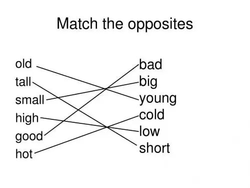
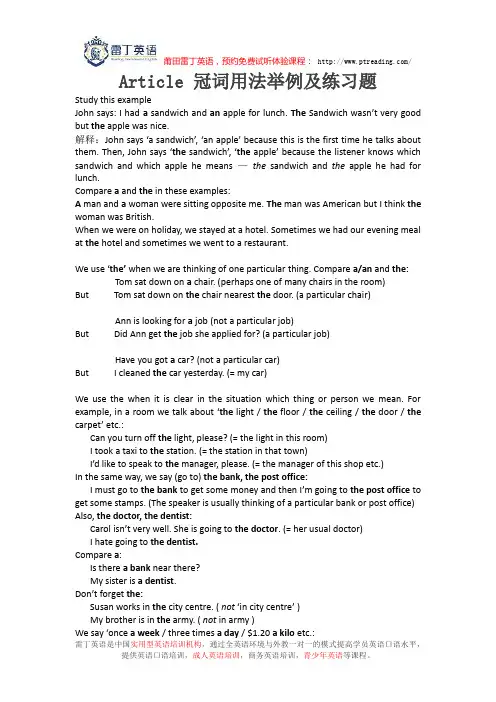
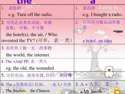
Article 冠词用法举例及练习题Study this exampleJohn says: I had a sandwich and an apple for lunch. The Sandwich wasn’t very good but the apple was nice.解释：John says ‘a sandwich’, ‘an apple’ because this is the first time he talks about them. Then, John says ‘the sandwich’, ‘the apple’ because the listener knows which sandwich and which apple he means —the sandwich and the apple he had for lunch.Compare a and the in these examples:A man and a woman were sitting opposite me. The man was American but I think the woman was British.When we were on holiday, we stayed at a hotel. Sometimes we had our evening meal at the hotel and sometimes we went to a restaurant.We use ‘the’ when we are thinking of one particular thing. Compare a/an and the: Tom sat down on a chair. (perhaps one of many chairs in the room)But Tom sat down on the chair nearest the door. (a particular chair)Ann is looking for a job (not a particular job)But Did Ann get the job she applied for? (a particular job)Have you got a car? (not a particular car)But I cleaned the car yesterday. (= my car)We use the when it is clear in the situation which thing or person we mean. For example, in a room we talk about ‘the light / the floor / the ceiling / the door / the carpet’ etc.:Can you turn off the light, please? (= the light in this room)I took a taxi to the station. (= the station in that town)I’d like to speak to the manager, please. (= the manager of this shop etc.)In the same way, we say (go to) the bank, the post office:I must go to the bank to get some money and then I’m going to the post office to get some stamps. (The speaker is usually thinking of a particular bank or post office) Also, the doctor, the dentist:Carol isn’t very well. She is going to the doctor. (= her usual doctor)I hate going to the dentist.Compare a:Is there a bank near there?My sister is a dentist.Don’t forget the:Susan works in the city centre. ( not‘in city centre’ )My brother is in the army. ( not in army )We say ‘once a week / three times a day / $1.20 a kilo etc.:How often do you go the cinema? About once a month.How much are those potatoes? $1.20 a kilo.She works eight hours a day, six days a week.Names with and without THEWe do not use ‘the’ with names of people ( Ann, Ann Taylor etc.). In the same way, we do not normally use ‘the’ with names of places. For example:Continents: Africa (not ‘the Africa’), Europe, South AmericaCountries: France (not ‘the France’), Japan, SwitzerlandStates, regions etc.: Texas, Central EuropeIslands: Corsica法国科西嘉岛，Sicily, BermudaCities, towns etc.: Cairo, New York, MadridMountains: Everest, KilimanjaroBut we use the in names with ‘Republic’, ‘Kingdom’, ‘States’ etc.:The United States of America the United Kingdom the Dominican RepublicThe People's Republic of ChinaWhen we use Mr / Mrs / Captain / Doctor ect. + a name, we do not use ‘the’. So we say:Mr. Johnson / Doctor Johnson / Captain Johnson / President Johnson etc. (not ‘the…’)Uncle Robert / Aunt Jane / Saint Catherine / Princess Anne etc. (not ‘the…’) Compare:We called the doctor. But We called Doctor Johnson. (not ‘the doctor Johnson’)We use mount (= mountain) and lake in the same way (without ‘the’)Mount Everest Lake SuperiorThey live near the lake. But They live near Lake Ontario.We use ‘the’with the names of oceans, seas, rivers and canalsThe Atlantic (Ocean) The Mediterranean (sea) the Red SeaThe Indian Ocean The Channel (Between France and Britain) the Suez CanalThe (River) Amazon The (River) Thames The Nile the Rhine Exercise: Put in a/an or the1 a. This house is very nice. Has it got____ garden?b. It’s a beautiful day. Let’s sit in_____ garden.c. I like living in this house but it’s a pity that______ garden is so small.2 a. Can you recommend ______ good restaurant?b. We had dinner in _____ very nice restaurant.c. We had dinner in _____ most expensive restaurant in town.3 a. She has ______ French name but in fact she’s English, not French.b. What’s ______ name of that man we met yesterday?c. We stayed at a very nice hotel —I can’t remember ____ name now.4 a. There isn’t _____ airport near where I live. _____ nearest airport is 70 milesaway.b. Our plane was delayed. We had to wait at _____ airport for three hours.c. Excuse me, please. Can you tell me how to get to _____ airport.访问页眉官网链接，通过网络渠道预约，即可获得免费英语体验课程。

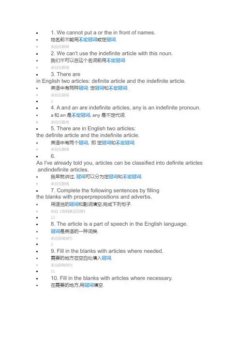
∙ 1. We cannot put a or the in front of names.∙姓名前不能用不定冠词或定冠词.∙来自互联网∙ 2. We can't use the indefinite article with this noun.∙我们不可以在这个名词前用不定冠词.∙来自互联网∙ 3. There arein English two articles: definite article and the indefinite article.∙英语中有两种冠词:定冠词和不定冠词.∙来自互联网∙2∙ 4. A and an are indefinite articles, any is an indefinite pronoun. ∙a和an是不定冠词,any是不定代词.∙来自互联网∙ 5. There are in English two articles:the definite article and the indefinite article.∙英语中有两个冠词, 即定冠词和不定冠词.∙来自互联网∙ 6.As I've already told you, articles can be classified into definite articles andindefinite articles.∙我早就讲过,冠词可以分为定冠词和不定冠词.∙来自互联网∙7. Complete the following sentences by fillingthe blanks with properprepositions and adverbs.∙用适当的冠词和副词填空,完成下列句子.∙来自《简明英汉词典》∙12∙8. The article is a part of speech in the English language.∙冠词是英语的一种词类.∙来自辞典例句∙2∙9. Fill in the blanks with articles where needed.∙需要的地方在空白处填入冠词.∙来自辞典例句∙51∙10. Fill in the blanks with articles where necessary.∙在需要的地方,用冠词填空.。

article英文作文格式1. I woke up late this morning, feeling groggy and disoriented. My alarm clock had failed me, leaving me scrambling to get ready for the day. I rushed through my morning routine, throwing on clothes and grabbing a quick breakfast. It was a chaotic start to the day, but I managed to make it out the door on time.2. As I walked to work, I noticed the sun shining brightly in the clear blue sky. The weather was perfect not too hot, not too cold. It put me in a good mood and made the walk more enjoyable. I couldn't help but smile as I passed by people on the street, feeling the warmth of the sun on my skin.3. When I arrived at the office, I was greeted by a mountain of paperwork on my desk. It seemed like there was no end to the tasks that needed to be completed. I took a deep breath and dove right in, determined to tackle each item one by one. The day was going to be busy, but I was upfor the challenge.4. During lunchtime, I decided to take a break and go for a walk outside. The fresh air and change of scenery helped clear my mind and recharge my energy. I strolled through the nearby park, admiring the colorful flowers and listening to the birds chirping. It was a peaceful moment amidst the chaos of the workday.5. Back at the office, I found myself in a meeting with my colleagues. We discussed upcoming projects and brainstormed ideas. It was a collaborative and productive session, with everyone sharing their thoughts and opinions.I enjoyed the lively discussion and felt inspired by the creativity in the room.6. As the workday came to a close, I felt a sense of accomplishment. Despite the challenges and busyness, I had managed to complete all my tasks. I packed up my things and headed home, looking forward to a relaxing evening.7. At home, I decided to unwind by watching a movie. Itwas a comedy that had me laughing out loud. The humor was a welcome distraction from the stresses of the day. I curled up on the couch with a bowl of popcorn, enjoying the movie and letting the laughter wash over me.8. Finally, it was time to go to bed. I crawled under the covers, feeling grateful for the day that had passed. It had been a rollercoaster of emotions, but ultimately a fulfilling and rewarding experience. As I closed my eyes, I looked forward to what tomorrow would bring.。