R语言DESeq 包介绍

【转录组⼊门】7：差异基因分析作业要求：使⽤R语⾔，载⼊表达矩阵，然后设置好分组信息，统⼀⽤DEseq2进⾏差异分析，当然也可以⾛⾛edgeR或者limma的voom流程。

基本任务是得到差异分析结果，进阶任务是⽐较多个差异分析结果的异同点。

【1】安装DESeq21 # 下⾯是在R语⾔中操作2 # 载⼊安装⼯具3 > source("/biocLite.R")4 # 安装包5 > biocLite("DESeq2")6 # 载⼊包7 > library("DESeq2")DESeq2对于输⼊数据的要求：1.DEseq2要求输⼊数据是由整数组成的矩阵。

2.DESeq2要求矩阵是没有标准化的。

【2】DESeq2进⾏差异表达分析DESeq2分析差异表达基因简单来说只有三步：构建dds矩阵，标准化，以及进⾏差异分析。

# dds <- DESeqDataSetFromMatrix(countData = cts, colData = coldata, design= ~ batch + condition) #~在R⾥⾯⽤于构建公式对象，~左边为因变量，右边为⾃变量。

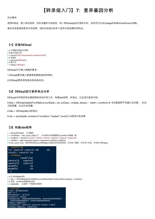
# dds <- DESeq(dds) #标准化# res <- results(dds, contrast=c("condition","treated","control")) #差异分析结果【3】构建dds矩阵1 > library(DESeq2) # 加载包2 > countData <- raw_count_filter[2:7] # 中括号中的数量要与condition中数量⼀致3 > condition <- factor(c("control","control","control","hypoxia","hypoxia","hypoxia"))4 > colData <- data.frame(s=colnames(countData),condition)5 # raw_count_filter：是所有样品的count按照gene id融合后⽣成的矩阵。

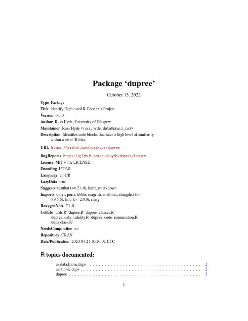
Package‘dupree’October13,2022Type PackageTitle Identify Duplicated R Code in a ProjectVersion0.3.0Author Russ Hyde,University of GlasgowMaintainer Russ Hyde<************************>Description Identifies code blocks that have a high level of similaritywithin a set of Rfiles.URL https:///russHyde/dupreeBugReports https:///russHyde/dupree/issuesLicense MIT+file LICENSEEncoding UTF-8Language en-GBLazyData trueSuggests testthat(>=2.1.0),knitr,rmarkdownImports dplyr,purrr,tibble,magrittr,methods,stringdist(>=0.9.5.5),lintr(>=2.0.0),rlangRoxygenNote7.1.0Collate'utils.R''dupree.R''dupree_classes.R''dupree_data_validity.R''dupree_code_enumeration.R''dups-class.R'NeedsCompilation noRepository CRANDate/Publication2020-04-2110:20:02UTCR topics documented:as.data.frame.dups (2)as_tibble.dups (2)dupree (3)12as_tibble.dups dupree_dir (4)dupree_package (5)EnumeratedCodeTable-class (5)print.dups (6)Index7 as.data.frame.dups as.data.frame method for‘dups‘classDescriptionas.data.frame method for‘dups‘classUsage##S3method for class dupsas.data.frame(x,...)Argumentsx any R object....additional arguments to be passed to or from methods.as_tibble.dups convert a‘dups‘object to a‘tibble‘Descriptionconvert a‘dups‘object to a‘tibble‘Usage##S3method for class dupsas_tibble(x,...)Argumentsx A data frame,list,matrix,or other object that could reasonably be coerced to a tibble....Other arguments passed on to individual methods.dupree3 dupree Detect code duplication between the code-blocks in a set offilesDescriptionThis function identifies all code-blocks in a set offiles and then computes a similarity score between those code-blocks to help identify functions/classes that have a high level of duplication,and could possibly be refactored.Usagedupree(files,min_block_size=40,...)Argumentsfiles A set offiles over which code-duplication should be measured.min_block_size dupree uses a notion of non-trivial symbols.These are the symbols/code-words that remain afterfiltering out really common symbols like<-,,,etc.Afterfiltering out these symbols from each code-block,only those blocks containingat least min_block_size symbols are used in the inter-block code-duplicationmeasurement....Unused at present.DetailsCode-blocks under a size threshold are disregarded before analysis(the size threshold is controlled by min_block_size);and only top-level code blocks are considered.Every sufficiently large code-block in the inputfiles will be present in the results at least once.If code-block X and code-block Y are present in a row of the resulting data-frame,then either X is the closest match to Y,or Y is the closest match to X(or possibly both)according to the similarity score;as such,some code-blocks may be present multiple times in the results.Similarity between code-blocks is calculated using the longest-common-subsequence(lcs)mea-sure from the package stringdist.This measure is applied to a tokenised version of the code-blocks.That is,each function name/operator/variable in the code blocks is converted to a unique integer so that a code-block can be represented as a vector of integers and the lcs measure is applied to each pair of these vectors.ValueA tibble.Each row in the table summarises the comparison between two code-blocks(block’a’and block’b’)in the inputfiles.Each code-block in the pair is indicated by:i)thefile(file_a/ file_b)that contains it;ii)its position within thatfile(block_a/block_b;1being thefirst code-block in a givenfile);and iii)the line where that code-block starts in thatfile(line_a/line_b).The pairs of code-blocks are ordered by decreasing similarity.Any match that is returned is either the top hit for block’a’or for block’b’(or both).4dupree_dirExamples#To quantify duplication between the top-level code-blocks in a fileexample_file<-system.file("extdata","duplicated.R",package="dupree")dup<-dupree(example_file,min_block_size=10)dup#For the block-pair with the highest duplication,we print the first four#lines:readLines(example_file)[dup$line_a[1]+c(0:3)]readLines(example_file)[dup$line_b[1]+c(0:3)]#The code-blocks in the example file are rather small,so if# min_block_size is too large,none of the code-blocks will be analysed#and the results will be empty:dupree(example_file,min_block_size=40)dupree_dir Run duplicate-code detection over all R-files in a directoryDescriptionRun duplicate-code detection over all R-files in a directoryUsagedupree_dir(path=".",min_block_size=40,filter=NULL,...,recursive=TRUE)Argumentspath A directory(By default the current working directory).Allfiles in this directory that have a".R",".r"or".Rmd"extension will be checked for code duplication.min_block_size dupree uses a notion of non-trivial symbols.These are the symbols/code-words that remain afterfiltering out really common symbols like<-,,,etc.Afterfiltering out these symbols from each code-block,only those blocks containingat least min_block_size symbols are used in the inter-block code-duplicationmeasurement.filter A pattern for use in grep-this is used to keep only particularfiles:eg,filter= "classes"would comparefiles with‘classes‘in thefilename ...Further arguments for grep.For example,‘filter="test",invert=TRUE‘would disregard allfiles with‘test‘in thefile-path.recursive Should we considerfiles in subdirectories as well?dupree_package5See Alsodupreedupree_package Run duplicate-code detection over allfiles in the‘R‘directory of apackageDescriptionThe function fails if the path does not look like a typical R package(it should have both an R/ subdirectory and a DESCRIPTIONfile present).Usagedupree_package(package=".",min_block_size=40)Argumentspackage The name or path to the package that is to be checked(By default the current working directory).min_block_size dupree uses a notion of non-trivial symbols.These are the symbols/code-words that remain afterfiltering out really common symbols like<-,,,etc.Afterfiltering out these symbols from each code-block,only those blocks containingat least min_block_size symbols are used in the inter-block code-duplicationmeasurement.See AlsodupreeEnumeratedCodeTable-classAn S4class to represent the code blocks as strings of integersDescriptionAn S4class to represent the code blocks as strings of integersSlotsblocks A tbl_df with columns‘file‘,‘block‘,‘start_line‘and‘enumerated_code‘6print.dups print.dups print method for‘dups‘classDescriptionprint method for‘dups‘classUsage##S3method for class dupsprint(x,...)Argumentsx an object used to select a method....further arguments passed to or from other methods.Indexas.data.frame.dups,2as_tibble.dups,2dupree,3dupree_dir,4dupree_package,5 EnumeratedCodeTable-class,5print.dups,67。

微生物群落组装过程 r语言微生物群落组装是指不同微生物个体在特定环境中相互作用并形成群落的过程。

R语言是一种功能强大的统计分析和可视化工具，可以用于微生物群落组装的研究。

以下是使用R语言进行微生物群落组装分析的一般步骤：1. 数据准备：将微生物群落数据整理成适合R语言处理的格式。

常见的数据格式包括OTU表（含有不同样本中各个OTU的丰度信息）和环境因子表（包含与微生物群落组成相关的环境因子数据）。

2. 数据预处理：根据需要对数据进行预处理，如去除低丰度的OTU、归一化样本间的差异等。

这可以使用R中的统计分析包进行操作，例如"vegan"、"phyloseq"等。

3. 多样性分析：使用R中的多样性分析包，如"vegan"和"phyloseq"，计算微生物群落的Alpha多样性（单样本内的物种多样性）和Beta多样性（样本间的物种多样性）。

4. 群落结构分析：使用R中的群落结构分析包，如"vegan"和"ade4"，可以进行聚类分析、主坐标分析（PCoA）等，以揭示样本间的群落结构差异。

5. 群落组装模型：使用R中的群落组装模型包，如"DESeq2"、"LEfSe"等，可以进行微生物群落组装的相关统计分析，并鉴定与环境因子显著相关的OTU或菌群。

6. 可视化：使用R中的可视化包，如"ggplot2"和"phyloseq"，绘制各种统计图表，如柱状图、热图、PCoA图等，以展示微生物群落的组成和结构。

需要注意的是，微生物群落组装是一个复杂的过程，涉及到多个环境因子和微生物个体之间的相互作用。

正确的数据处理和分析方法对于结果的解释和解读至关重要。

因此，在使用R语言进行微生物群落组装研究时，建议参考相关文献和专业指导，确保分析方法的准确性和可靠性。

【R】R语⾔常⽤包汇总⼀、⼀些函数包⼤汇总时间上有点过期，下⾯的资料供⼤家参考基本的R包已经实现了传统多元统计的很多功能，然⽽CRNA的许多其它包提供了更深⼊的多元统计⽅法，下⾯要综述的包主要分为以下⼏个部分：1）多元数据可视化（Visualising multivariate data）绘图⽅法 基本画图函数（如：pairs()、coplot()）和 lattice包⾥的画图函数（xyplot()、splom()）可以画成对列表的⼆维散点图，3维密度图。

car 包⾥的scatterplot.matrix()函数提供更强⼤的⼆维散点图的画法。

cwhmisc包集合⾥的cwhplot包的pltSplomT()函数类似pair()画散点图矩阵，⽽且可以在对⾓位置画柱状图或密度估计图。

除此之外，scatterplot3d包可画3维的散点图，aplpack包⾥bagplot()可画⼆变量的boxplot，spin3R()可画可旋转的三维点图。

misc3d包有可视化密度的函数。

YaleToolkit包提供许多多元数据可视化技术，agsemisc也是这样。

更特殊的多元图包括：aplpack包⾥的faces()可画Chernoff’s face；MASS包⾥的parcoord()可画平⾏坐标图（矩阵的每⼀⾏画⼀条线，横轴表⽰矩阵的每列）； graphics包⾥的stars()可画多元数据的星状图（矩阵的每⼀⾏⽤⼀个星状图表⽰）。

ade4包⾥的mstree()和vegan包⾥的spantree()可画最⼩⽣成树。

calibrate包⽀持双变量图和散点图，chplot包可画convex hull图。

geometry包提供了和qhull库的接⼝，由convexhulln()可给出相应点的索引。

ellipse包可画椭圆，也可以⽤plotcorr()可视化相关矩阵。

denpro包为多元可视化提供⽔平集树形结构（level set trees）。

基因组学数据分析中差异表达分析的使用方法差异表达分析是基因组学研究中常用的一种分析方法，用于比较不同条件或样本之间基因表达的差异。

这种分析方法可以帮助研究人员理解基因表达调控的机制、寻找与特定疾病相关的基因、发现新的分子标记物等。

本文将介绍差异表达分析的基本流程和相关的工具。

差异表达分析的基本流程通常包括：数据预处理、差异基因筛选和分析结果的验证。

首先，进行数据预处理，主要包括原始数据的读取、质量控制和归一化等。

其次，进行差异基因筛选，通过统计学方法或基因表达差异的幅度和显著性来确定差异基因。

最后，对选定的差异基因进行验证，可以使用实验室实验技术如RT-PCR、Western blot 等，或者进行功能富集分析、通路分析等。

在进行差异表达分析时，研究人员通常会使用一些专门的工具和软件。

下面以DESeq2为例，介绍差异表达分析的具体步骤。

首先，将原始数据导入到R或Python等编程环境中，利用相应的包或库进行数据预处理。

DESeq2是R语言中最常用的差异表达分析工具之一。

它可以处理RNA-seq数据，对基因表达的差异进行统计显著性分析。

使用DESeq2进行数据预处理时，首先需要进行数据的归一化处理，通常使用RPKM（reads per kilobase of exon per million mapped reads）或TPM（Transcripts Per Kilobase Million）方法将数据进行归一化处理。

接下来，进行差异基因筛选。

DESeq2使用负二项分布模型对差异表达进行建模，通过p值和调整的p值来判断差异的显著性。

DESeq2还结合了前沿理论来估计基因表达的离散性，提高了差异表达分析的准确性。

通过设定阈值，筛选出显著差异表达的基因。

此外，DESeq2还可以计算基因的表达倍数差异，帮助研究人员判断差异的生物学意义。

最后，对差异基因进行验证。

一种常用的验证方法是使用实验室技术如RT-PCR，验证差异基因在不同条件或样本中的表达水平。

转录组分析_R范文转录组分析是利用高通量测序技术对细胞或组织的所有转录本进行检测和定量的一种方法。

由于转录组包含了所有的转录本信息，因此转录组分析可以帮助我们了解基因的表达模式、功能注释以及基因调控网络等重要信息。

在转录组研究中，R语言是一个广泛应用的工具，用于数据分析和可视化。

下面是一些常见的R语言在转录组分析中的应用：1. 数据预处理：在进行转录组分析之前，我们需要对原始测序数据进行预处理。

这包括质量控制、去除低质量读段和适配序列以及对数据进行过滤和修剪。

R语言提供了许多用于转录组数据预处理的包，例如“ShortRead”和“fastqcr”等。

2. 差异表达基因分析：差异表达基因分析是转录组研究中最常见的任务之一、通过比较不同条件下的基因表达水平，我们可以识别特异表达的基因，并了解它们在生物过程中的功能。

在R语言中，可以使用各种包进行差异表达基因分析，例如“DESeq2”和“limma”等。

3. 功能注释和富集分析：功能注释和富集分析帮助我们理解差异表达基因的生物学功能。

R语言提供了许多包用于进行功能注释和富集分析，例如“clusterProfiler”和“enrichR”等。

这些包可以根据基因的注释信息，并通过各种数据库进行富集分析，例如基因本体论（Gene Ontology，GO）和KEGG等。

4. 转录因子识别和调控网络分析：在转录组分析中，我们还可以通过分析差异表达基因的共享调控因子来研究基因调控网络。

R语言提供了一些用于识别转录因子结合位点的包，例如“ChIPseeker”和“findPeaks”等。

此外，通过整合转录组数据和转录因子结合位点信息，可以构建基因调控网络并进行网络分析。

5. 可视化：数据可视化对于转录组分析来说非常重要，可以帮助我们更直观地理解数据和结果。

R语言提供了许多绘图包用于转录组数据的可视化，例如“ggplot2”和“pheatmap”等。

这些包可以生成各种图表，包括热图、散点图和折线图等。

r语言数据标准化在数据分析中，数据标准化是一个非常重要的步骤。

它可以帮助我们消除不同变量之间的量纲影响，使得数据更加可比较和可解释。

在R语言中，数据标准化可以通过多种方法实现，本文将介绍一些常用的数据标准化方法，并给出在R语言中的具体实现步骤。

一、Z-score标准化。

Z-score标准化是一种常用的数据标准化方法，它通过将原始数据减去均值，再除以标准差的方式来实现。

在R语言中，可以使用如下代码来对数据进行Z-score标准化：```R。

# 假设data为需要标准化的数据框。

data_standardized <scale(data)。

```。

这段代码中，scale()函数可以对数据进行Z-score标准化，得到的data_standardized即为标准化后的数据。

二、Min-max标准化。

Min-max标准化是另一种常用的数据标准化方法，它通过将原始数据减去最小值，再除以最大值和最小值之差的方式来实现。

在R语言中，可以使用如下代码来对数据进行Min-max标准化：```R。

# 假设data为需要标准化的数据框。

data_standardized <apply(data, 2, function(x) (x min(x)) / (max(x) min(x)))。

```。

这段代码中，apply()函数可以对数据进行Min-max标准化，得到的data_standardized即为标准化后的数据。

三、小数定标标准化。

小数定标标准化是另一种常用的数据标准化方法，它通过将原始数据除以一个适当的基数（10的幂次方）来实现。

在R语言中，可以使用如下代码来对数据进行小数定标标准化：```R。

# 假设data为需要标准化的数据框。

data_standardized <apply(data, 2, function(x) x /10^ceiling(log10(max(abs(x)))))。

```。

dep包蛋白组学一、引言随着生物信息学的发展，dep包作为一种高效、精确的蛋白质组学数据分析工具，逐渐在科研领域崭露头角。

本文将从dep包的作用、基本原理、应用案例、优缺点分析、使用方法与技巧等方面进行介绍，以期帮助读者更好地应用dep包开展蛋白质组学研究。

dep包，全称为“DESeq2”，是由Rossettini等人于2012年开发的一种基于RNA测序数据的差异表达分析工具。

近年来，随着质谱技术在蛋白质组学领域的广泛应用，dep包也被成功地应用于蛋白质组学数据分析。

通过对蛋白质表达量的精确测量和差异分析，dep包为研究者揭示了生物过程中的分子机制，为疾病诊断、治疗和预防提供了新的思路。

二、dep包的基本原理dep包基于RNA测序数据进行蛋白质组学分析，其主要原理包括以下两个方面：1.算法原理：dep包采用了一种基于负log似然估计的方法（LDA），将原始测序数据转化为蛋白质表达量估计值。

通过对比不同样本间的表达量差异，dep包可以识别出差异表达的蛋白质。

2.数据处理流程：首先，将原始质谱数据进行预处理，包括峰识别、峰匹配、定量等步骤；然后，利用dep包进行差异表达分析；最后，对分析结果进行统计检验和可视化展示。

三、dep包在蛋白组学分析中的应用案例1.蛋白质定量：dep包可以对蛋白质进行定量分析，从而为研究者提供有关生物过程中蛋白质表达变化的信息。

2.差异表达分析：通过对比不同样本或处理组的蛋白质表达量，dep包可以识别出差异表达的蛋白质，为进一步的生物实验和功能研究提供依据。

3.蛋白质相互作用网络构建：dep包可以结合其他生物信息学工具，如Cytoscape等，构建蛋白质相互作用网络，揭示生物体内的分子调控机制。

四、dep包的优缺点分析1.优点：（1）高效：dep包可以快速处理大量蛋白质组数据；（2）精确：dep包对蛋白质表达量的估计具有较高的准确性；（3）可靠性：dep包的结果经过统计检验，具有较高的可靠性。

Bioconductor包的使用方法1. 什么是Bioconductor包？Bioconductor是一个用于生物信息学和计算生物学的开源软件项目，旨在提供生物学数据的分析和可视化工具。

Bioconductor项目提供了大量的R语言包，用于处理、分析和可视化生物学数据。

这些包涵盖了多个领域，包括基因表达、基因组学、蛋白质组学、代谢组学等。

Bioconductor包的使用方法可以帮助生物学家、生物信息学家和计算生物学家更好地利用Bioconductor项目提供的工具和资源，进行生物学数据的分析和解释。

2. 安装Bioconductor包要使用Bioconductor包，首先需要安装Bioconductor。

安装Bioconductor的方法如下：if (!requireNamespace("BiocManager", quietly = TRUE))install.packages("BiocManager")BiocManager::install()上述代码会安装BiocManager包，然后使用BiocManager::install()函数安装Bioconductor。

3. 查找Bioconductor包Bioconductor提供了一个网站，可以用于查找和浏览Bioconductor包。

该网站的网址是，可以在搜索框中输入关键词来查找相关的包。

在R中，可以使用BiocManager::available()函数来列出所有可用的Bioconductor 包。

可以使用BiocManager::search()函数来搜索包含指定关键词的包。

# 列出所有可用的Bioconductor包BiocManager::available()# 搜索包含指定关键词的Bioconductor包BiocManager::search("gene expression")4. 安装Bioconductor包要安装Bioconductor包，可以使用BiocManager::install()函数。

导出差异基因的表达矩阵r语言在R语言中，差异基因表达分析是生物信息学领域的常见任务。

差异基因表达矩阵通常包含基因在不同条件下的表达水平，并且已经过统计测试来识别表达显著差异的基因。

以下是使用R 语言导出差异基因表达矩阵的基本步骤：1.数据导入与预处理：首先，你需要将基因表达数据导入R中。

这些数据通常以表格形式存在，如CSV或TSV文件。

你可以使用read.csv()或read.delim()函数来导入数据。

2.数据格式化：确保数据以适当的格式进行组织，通常是一个矩阵或数据框（data.frame），其中行代表基因，列代表样本或条件。

3.差异表达分析：使用适当的统计方法（如t检验、DESeq2、edgeR等）来分析基因在不同条件下的表达差异。

这些方法通常需要你将数据分组为比较的条件。

4.提取差异基因：根据统计测试的结果，提取显著差异表达的基因。

这通常涉及设置一个显著性阈值（如p值<0.05）和/或一个表达变化阈值（如log2倍数变化>1或<-1）。

5.导出差异基因表达矩阵：创建一个新的数据框或矩阵，其中包含显著差异基因的表达数据，并使用write.csv()或类似的函数将其导出为CSV文件。

以下是一个简化的示例代码，展示了这些步骤的基本框架：R# 1. 数据导入expression_data <- read.csv("gene_expression_data.csv", s = 1)# 2. 数据预处理（如果需要）# ...# 3. 差异表达分析（这里使用假设的函数进行演示）# 假设你已经有了条件分组信息，如条件A和条件Bcondition <- factor(c(rep("A", 3), rep("B", 3))) # 示例条件向量diff_expression_results <-perform_differential_expression_analysis(expression_data, condition)# 4. 提取差异基因# 假设diff_expression_results包含p值和log2倍数变化等信息significant_genes <-diff_expression_results[diff_expression_results$p_value < 0.05 &abs(diff_expression_results$log2FC) > 1,]# 5. 导出差异基因表达矩阵# 这里我们只导出显著差异基因的原始表达数据significant_gene_expression <-expression_data[rownames(significant_genes),]write.csv(significant_gene_expression,"significant_gene_expression_matrix.csv")请注意，上面的代码是一个框架示例，并不包含实际的差异表达分析函数（如perform_differential_expression_analysis），因为这需要根据你的具体数据和所使用的包来定制。

de_workflow_salmon_deseq1.png sc_DE_dispersion.pngsc_DE_res_tbl.png sc_DE_sig_res.pngsc_DE_top20.pngsc_DE_sig_genes_heatmap.png sc_DE_volcano.pngdir.create("DESeq2")dir.create("DESeq2/pairwise")# Function to run DESeq2 and get result s for all clusters## x is index of cluster in clusters vector on which to run function## A is the s ample group to compare## B is the sample group to compare against (base level)get_dds_r esultsAvsB <- function(x, A, B){ cluster_metadata <- metadata[which(metadata$cluster_id == clusters[x]), ] rownam es(cluster_metadata) <- cluster_metadata$sample_id counts <- pb[[clusters[x]]] clust er_counts <- data.frame(counts[, which(colnames(counts) %in% rownames(cluster_metadat a))]) #all(rownames(cluster_metadata) == colnames(cluster_counts)) d ds <- DESeqDataSetFromMatrix(cluster_counts, colData = cluster_me tadata, design = ~ group_id) # Transform counts for data visua lization rld <- rlog(dds, blind=TRUE) # Plot PCA DESeq2::plotPCA(rld, intgroup = "group_id") ggsave(paste0("results/", clusters[x], "_specific_PCAplot.png")) # Extract the rlog matrix from the object and compute pairwise correlation values rld_mat <- assay(rld) rld_cor <- cor(rld_mat) # Plot heatmap png(paste0( "results/", clusters[x], "_specific_heatmap.png")) pheatmap(rld_cor, annotation = cluster_ metadata[, c("group_id"), drop=F]) dev.off() # Run DESeq2 differential expressi on analysis dds <- DESeq(dds) # Plot dispersion estimates png(paste0("res ults/", clusters[x], "_dispersion_plot.png")) plotDispEsts(dds) dev.off() # Output re sults of Wald test for contrast for A vs B contrast <- c("group_id", levels(cluster_metadata $group_id)[A], levels(cluster_metadata$group_id)[B]) # resultsNames(dds) res <- results(dds, contrast = contrast, alpha = 0.05) res <- lfcShrink(dds, contrast = contrast, res=res) # Set thresholds padj_cutoff <- 0.05 # Turn the results obje ct into a tibble for use with tidyverse functions res_tbl <- res %>% data.frame() %>% rownames_to_column(var="gene") %>% as_tibble() write.cs v(res_tbl, paste0("DESeq2/pairwise/", clusters[x], "_", levels(cluster_metadata$gro up_id)[A], "_vs_", levels(cluster_metadata$group_id)[B], "_all_genes.csv"), quote = FALSE, s = FALSE) # Subset the significant results sig_res <- dplyr::filter(res_tbl, padj < padj_cutoff) %>% dplyr::arrange(padj) write.csv(sig_res, paste0("DESeq2/pairwise/", cl usters[x], "_", levels(cluster_metadata$group_id)[A], "_vs_", levels(cluster_metadata$group_id)[B], "_sig_genes.csv"), quote = FALSE, s = FALSE) # # ggplot of top genes normalized_counts <- counts(dds, normalized = TRUE) ## Order results by padj values top20_sig_genes <- sig_res %>% dplyr::arrange(padj) %>% dplyr::pull(gene) %>% head(n=20) top20_sig_norm <- data.frame(normalized_counts) %>% rownames_to_column( var = "gene") %>% dplyr::filter(gene %in% top20_sig_genes) gathered_top 20_sig <- top20_sig_norm %>% gather(colnames(top20_sig_norm)[2:length(colnames(top20_sig_norm))], key = "samplename", value = "normalized_counts") gathered_top20_sig <- inner_join(ei[, c("sample_id", "group_id" )], gathered_top20_ sig, by = c("sample_id" = "samplename")) ## plot using ggplot2 ggplot(gathered _top20_sig) + geom_point(aes(x = gene, y = normalized_counts, color = group_id), position=position_jitter(w=0.1,h=0)) + scale_y_log10() + xlab("Genes") + ylab("log10 Normalized Counts") + ggtitle("Top 20 Significant DE Genes") + theme_bw() + theme(axis. text.x = element_text(angle = 45, hjust = 1)) + theme(plot.title = element_text(hjust = 0.5)) ggsave(paste0("DESeq2/pairwise/", clusters[x], "_", levels(cluster_metadata$grou p_id)[A], "_vs_", levels(cluster_metadata$group_id)[B], "_top20_DE_genes.png")) }# Run the script on all clusters comparing stim condition relative to control conditionmap(1:length(clusters), get_dds_resultsAvsB, A = 2, B = 1)Script to run DESeq2 on all cell type clusters - Likelihood Ratio TestThe following script will run the DESeq2 Likelihood Ratio Test (LRT) on all cell type clusters. This script can easily be run on the cluster for fast and efficient execution and storage of results.# Likelihood ratio testdir.c reate("DESeq2/lrt")# Create DESeq2Dataset objectclusters <- levels(metadata$cluster_id)m etadata <- gg_df %>% select(cluster_id, sample_id, group_id) metadata$group <- paste 0(metadata$cluster_id, "_", metadata$group_id) %>% factor()# DESeq2library(DEGrepo rt)get_dds_LRTresults <- function(x){ cluster_metadata <- metadata[which(metadata$cluster_id == clusters[x]), ] row names(cluster_metadata) <- cluster_metadata$sample_id counts <- pb[[clusters[x]]] cluster_counts <- data.frame(counts[, which(colnames(counts) %in% rownames(cluster_met adata))]) #all(rownames(cluster_metadata) == colnames(cluster_counts)) dds <- DESeqDataSetFromMatrix(cluster_counts, colData = cluster _metadata, design = ~ group_id) dds_lrt <- DESeq(dds, test=" LRT", reduced = ~ 1) # Extract results res_LRT <- results(dds_lrt) # Cre ate a tibble for LRT results res_LRT_tb <- res_LRT %>% data.frame() %>% rownames_to_column(var="gene") %>% as_tibble() # Save all results write.csv(res_LRT_tb, paste0("DESeq2/lrt/", clusters[x], "_LRT_all_genes.csv "), quote = FALSE, s = FALSE) # Subset to return gen es with padj < 0.05 sigLRT_genes <- res_LRT_tb %>% filter(padj < 0.05) # Save sig results write.csv(sigLRT_genes, paste0("DESeq2/lrt/", clusters[x ], "_LRT_sig_genes.csv"), quote = FALSE, s = FALSE) # Transform counts for data visualization rld <- rlog(dds_lrt, blind=TRUE) # Ex tract the rlog matrix from the object and compute pairwise correlation values rld_mat <- a ssay(rld) rld_cor <- cor(rld_mat) # Obtain rlog values for those significant ge nes cluster_rlog <- rld_mat[sigLRT_genes$gene, ] cluster_meta_sig <- cluster_ metadata[which(rownames(cluster_metadata) %in% colnames(cluster_rlog)), ] # # Remove samples without replicates # cluster_rlog <- cluster_rlog[, -1] # cluster_metadata <- cluster_metadata[which(rownames(cluster_metadata) %in% co lnames(cluster_rlog)), ] # Use the `degPatterns` function from the 'DEGreport' p ackage to show gene clusters across sample groups cluster_groups <- degPatterns(clus ter_rlog, metadata = cluster_meta_sig, time = "group_id", col=NULL) ggsave(paste0("D ESeq2/lrt/", clusters[x], "_LRT_DEgene_groups.png")) # Let's see what is stored in t he `df` component write.csv(cluster_groups$df, paste0("DESeq2/lrt/", clusters[ x], "_LRT_DEgene_groups.csv"), quote = FALSE, s = FALSE) saveRDS(cluster_groups, paste0("DESeq2/lrt/", clusters[x], "_LRT_DEgene_group s.rds")) save(dds_lrt, cluster_groups, res_LRT, sigLRT_genes, file = paste0("DESeq2/lrt /", clusters[x], "_all_LRTresults.Rdata")) }map(1:length(clusters), get_dds_LRTresults)完!!!注：以上内容来⾃哈佛⼤学⽣物信息中⼼(H B C)_的教学团队的⽣物信息学培训课程。

R语言包的安装载入及使用方法R语言是一种广泛使用的统计分析工具和编程语言，它提供了许多功能强大的包来进行数据处理、统计分析、可视化等工作。

本文将介绍如何安装、加载和使用R语言包。

一、安装R语言包例如，要安装包`dplyr`，可以执行以下代码：```Rinstall.packages("dplyr")```当然，也可以同时安装多个包，只需将包的名称用逗号隔开即可：```Rinstall.packages(c("dplyr", "ggplot2"))```在安装包时，通常会提示选择一个CRAN镜像站点，可以选择离自己地理位置最近的一个站点，或者根据网络速度选择一个较快的站点。

二、加载R语言包一般来说，包在安装后并没有自动加载到R的环境中，需要使用`library(`函数来手动加载包。

该函数的参数是要加载的包的名称（或多个包的名称）。

例如，要加载包`dplyr`，可以执行以下代码：library(dplyr)```同样，可以同时加载多个包，只需将包的名称用逗号隔开即可：```Rlibrary(dplyr, ggplot2)```三、使用R语言包加载完R语言包后，就可以使用其中的函数和数据了。

一般来说，包会提供一些函数和数据集，可以使用`?`符号来查看包的帮助文档和使用示例。

例如，要查看包`dplyr`的帮助文档，可以执行以下代码：```Rdplyr```帮助文档会显示包的详细介绍、函数列表和使用示例等内容。

可以根据需要查看和学习。

此外，还可以通过`data(`函数来查看包中包含的数据集。

该函数的参数是数据集的名称。

例如，要查看包`dplyr`中包含的数据集`mpg`，可以执行以下代码：data(mpg)```执行后，数据集`mpg`就会被加载到全局环境中，可以直接使用。

在使用包的函数时，一般需要先使用包名加上函数名的方式进行调用。

例如，要使用`dplyr`包中的`filter(`函数来过滤数据，可以执行以下代码：```Rdplyr::filter(mpg, manufacturer == "audi")```上述代码会对数据集`mpg`进行过滤，只保留制造商为"Audi"的数据。

r语言基因id转换R语言是一门非常强大的统计分析语言，广泛应用于生物信息学领域。

在进行生物学数据分析时，我们经常需要将各种ID之间进行转换，如转换基因ID、转换蛋白质ID等。

本文将介绍如何使用R语言进行基因ID的转换。

首先，我们需要导入所需的R包。

在进行基因ID转换时，我们通常需要使用“biomart”包和“AnnotationDbi”包。

在R中安装这两个包的命令如下：```Rinstall.packages("biomart")install.packages("AnnotationDbi")```安装完这两个包后，我们就可以使用它们提供的函数进行基因ID转换了。

以将Ensembl基因ID转换为HGNC基因符号为例，我们可以使用以下代码：library(biomart)library(AnnotationDbi)ensembl <- useMart("ENSEMBL_MART_ENSEMBL", dataset = "hsapiens_gene_ensembl")annotations <- select(ensembl, attributes =c("ensembl_gene_id", "hgnc_symbol"),filter = "ensembl_gene_id", values = gene_ids)# 下面这一步就是为了去除基因id转换过程中出现的NA值annotations <- na.omit(annotations)```其中，我们首先使用“useMart”函数连接到Ensembl数据库。

然后，使用“select”函数指定需要查询的属性和过滤条件。

最后，我们通过“na.omit”函数去除转换过程中出现的NA值，以保证最终的结果是完整的。

deseq2方法描述
DESeq2是一种用于RNA测序数据分析的统计学方法，它被广泛用于发现基因表达水平在不同条件下的差异。

DESeq2主要用于识别不同实验条件下基因表达的差异，例如对疾病和对照组的比较。

DESeq2的方法主要包括数据预处理、差异表达分析和结果解释等步骤。

首先，在数据预处理阶段，DESeq2会对原始的RNA测序数据进行质量控制和归一化处理，以保证数据的准确性和可靠性。

接着，在差异表达分析阶段，DESeq2使用负二项分布模型来对基因表达水平进行建模，并计算出每个基因在不同条件下的表达差异。

DESeq2还考虑了数据中的离散性和过度离群值的影响，提高了对低表达基因和小样本量数据的分析效果。

最后，在结果解释阶段，DESeq2会生成差异表达基因列表和统计学上的显著性水平，帮助研究人员识别和理解不同实验条件下基因表达的差异。

此外，DESeq2还提供了可视化工具，如热图和散点图，帮助研究人员直观地展示和解释数据分析结果。

总的来说，DESeq2方法通过严谨的统计学模型和全面的数据处
理流程，能够准确地识别RNA测序数据中的差异表达基因，为基因表达调控和疾病机制研究提供了重要的分析工具。