Network4611_user_guide

1.4G运营商支持：联通、电信、移动
2.系统自动识别SIM卡，不要带电插拔SIM卡(插拔SIM卡，建议断电操作)
3.4G支持的版本：MIG
4.3R2
4.4G的硬件型号只有一个:MIG-1250-LTE
5.支持专线，但是需要专线卡，以及专线的APN/用户名/密码
6.模式:
A.4g优先:开机后根据网络好坏自动搜网,搜网顺寻4G->3G->2G;
有这么个情况，如果当前自动模式在3G网络，且设备与外网有数据交互，
则此时及时4G网络信号变好也不会马上变为4G
B.3g优先:开机后根据网络好坏自动搜网,搜网顺寻3G->4G;
C.仅4G:只搜4G网络。

注:如果SIM卡没有费用，则注册不了4G信号。

7.常见问题检测（复制自页面”常见故障排查”）:
拨号失败的排查步骤:
1.首先确定设备所在的范围是否有覆盖4G/3G网络.
这个是前提条件.
2.首先检测信号、网络注册模式.
通过"刷新状态"来获取当前的信号,和网络注册模式,确定网络注册成功.
3.接着检测APN,用户名,密码,认证方式的配置.
确定拨号参数、拨号模式符合拨号预期.
如果电信3G模式下使用默认的用户名密码拨号不上,可将用户名/密码分别修改为ctnet@/vnet.mobi进行尝试.
4.确定SIM卡是否欠费.
SIM卡欠费后,是注册不了4G网络,或者根本注册不了网络.
目前发现的欠费现象有:
a.欠费的电信4G卡,只能注册到3G的网络.
b.欠费的移动4G卡,只能注册到3G的网络,且拨上号不能获取到DNS.。

浪潮英信服务器BIOS用户手册文档版本V2.2 发布日期2022-10-12版权所有© 2021-2022浪潮电子信息产业股份有限公司。

保留一切权利。

未经本公司事先书面许可，任何单位和个人不得以任何形式复制、传播本手册的部分或全部内容。

环境保护请将我方产品的包装物交废品收购站回收利用，以利于污染预防，共同营造绿色家园。

商标说明Inspur浪潮、Inspur、浪潮、英信是浪潮集团有限公司的注册商标。

本手册中提及的其他所有商标或注册商标，由各自的所有人拥有。

内容声明您购买的产品、服务或特性等应受浪潮集团商业合同和条款的约束。

本文档中描述的全部或部分产品、服务或特性可能不在您的购买或使用范围之内。

除非合同另有约定，浪潮集团对本文档的所有内容不做任何明示或默示的声明或保证。

文档中的示意图与产品实物可能有差别，请以实物为准。

本文档仅作为使用指导，不对使用我们产品之前、期间或之后发生的任何损害负责，包括但不限于利益损失、信息丢失、业务中断、人身伤害，或其他任何间接损失。

本文档默认读者对服务器产品有足够的认识，获得了足够的培训，在操作、维护过程中不会造成个人伤害或产品损坏。

文档所含内容如有升级或更新，恕不另行通知。

技术支持客户服务电话：4008600011地址：中国济南市浪潮路1036号浪潮电子信息产业股份有限公司邮箱：***************邮编：250101前言摘要本手册介绍服务器BIOS设置的相关内容。

目标受众本手册主要适用于以下人员：●技术支持工程师●产品维护工程师建议由具备服务器知识的专业工程师参考本手册进行服务器运维操作。

符号约定在本文中可能出现下列标志，它们所代表的含义如下。

图标说明如不当操作，可能会导致死亡或严重的人身伤害。

如不当操作，可能会导致中度或轻微的人身伤害。

如不当操作，可能会导致设备损坏或数据丢失。

为确保设备成功安装或配置，而需要特别关注的操作或信息。

对手册内容的描述进行必要的补充和说明。

4G LTE Modem Data SheetLB1111Highlights• Simple LTE connectivity solution• 4G LTE speeds up to 150 Mbps downloads and 50 Mbps uploads• 3G/2G fallback support• Manage settings via a browser-based web UIOverviewThe NETGEAR 4G LTE Modem gives you a simple, LTE connectivity solution for your devices, avoiding disruptions in broadband when your fixed wire line goes down. Simply connect this modem directly to your router, switch or computer to provide an automatic 4G LTE or 3G/2G broadband backup connection with download speeds of up to 150 Mbps. It has a Gigabit Ethernet WAN port so that you can plug in your wireless router and share connection with all your Wi-Fi and wired devices. In addition, this LTE modem comes with Power-over-Ethernet for remote locations. The NETGEAR 4G LTE Modem is also compact, convenient, and simple to setup.Key FeaturesSuper-fast Connectivity with 4G LTE & 3GGet secure and super-fast 4G LTE connectivity with 3G/2G fallback for broadband failover. Get up to 150 Mbpsdownload and 50 Mbps upload speeds.Wired ConnectionsGigabit Ethernet WAN port for connection pass-through. Power-over-Ethernet for remote locations.Better Signal ReceptionTwo connectors available to connect optional 4G/3G antennas for better signal reception.SCAN T O LEARN MORE4G LTE Modem Data SheetLB1111 Use CasesWe all depend on a fast, always-on broadband connection, and planning ahead to ensure everyone stays connected is essential.The NETGEAR 4G LTE Modem is a reliable backup source for broadband connectivity, allowing you to continue running without any disruptionwhen your wire line broadband is unexpectedly not available.Using the NETGEAR 4G LTE Modem for broadband connectivity enables Internet access at fast speeds with the convenience of portabilityand flexibility. Unlike other connectivity sources, the NETGEAR 4G LTE Modem can be easily installed in a matter of minutes, and it's idealfor a wide range of environments including rural areas, outdoors, and locations where wireline option is not readily available. Power-over-Ethernet adds a powering option for remote locations. Some typical applications include:• LTE WAN backup for business continuity• Interim solution to fixed line service• Last-mile connection• Kiosk - wire-free connection• Vacation cabins / rural homes• Temporary offices such as construction sites• Mobile stores such as food trucks4G LTE ModemData SheetLB1111This product comes with a limited warranty that is valid only if purchased from a NETGEAR authorised reseller.*90-day complimentary technical support following purchase from a NETGEAR authorised reseller.ATTENTION: Due to EU law, the country settings must be identical to the country where the device is operating (important due to non-harmonised frequencies in the EU.)For indoor use only.Valid for sale in all EU member states, EFTA states, and Switzerland.NETGEAR, the NETGEAR Logo, and AirCard are trademarks of NETGEAR, Inc. in the United States and/or other countries. Other brand names mentioned herein are for identification purposes only and may be trademarks of their respective holder(s). Information is subject to change without notice. ©2016 NETGEAR, Inc. All rights reserved.NETGEAR, Inc. 350 E. Plumeria Drive, San Jose, CA 95134-1911 USA, NETGEAR INTL LTD, Building 3, University Technology Centre, Curraheen Road, Cork, Ireland, /support D-L B1111-1Package Contents• 4G LTE Modem (LB1111)• Power adapter • Ethernet cable • Quick start guideSpecifications• Dimensions: 120 (W) x 99 (D) x 31 (H) mm • Weight: 200 gBand Support• LTE Category 4 (up to 150 Mbps): B3, 7, 8, 20, 40• UMTS DC-HSPA+ - (up to 42 Mbps): B1, 8• Quad band GSMInterface• 1 Gigabit WAN Ethernet RJ-45 port (PoE)• I nternal WWAN antennas with support foroptional TS9 external antennas • 3FF (micro) SIM card slotLEDs• Power• LTE Signal Quality (5 LED bar graph)• LANPower Adapter• 12V DC, 1AKey Features• B uilt-in Gigabit WAN connection for flexible home and office connectivity• F ast 4G LTE backup speeds up to 150 Mbps for downloads and 50 Mbps for uploads • Provides 4G to 3G fallback support • Power-over-Ethernet• S MS message alerts for firmware updates, data usage, and failover to LTE • TR-069 for remote management• T wo TS-9 connectors available to connect optional 4G/3G antennas for better signal reception• D irect IP pass-through for secure enterprise VPN configuration• Manage settings via a browser-based web UI • L EDs on device to check network status instantly• P ortable, light and compact design for you to take anywhereSystem Requirements• C ompatible 2G/3G/4G LTE Mobile Service (3FF Micro-SIM)• M icrosoft Windows 7, 8, 8.1, 10, Vista, XP, Mac OS ® (10.6.8. and newer) and other operating systems running a TCP/IP network (foraccessing Web Management User Interface)• C ompatible browsers such as Microsoft ® Internet Explorer ® 5.0, Firefox ® 2.0, Safari ® 1.4, or Google Chrome ™ 11.0 browsers or higher (for accessing Web Management User Interface)Support• 90-day complimentary technical support*Warranty• /warrantyAntenna ConnectorPower ConnectorPower SwitchReset ButtonGigabit WANPort Antenna Connector。

浪潮以太网交换机命令手册系统分册前言 (13)1配置基础命令 (16)1.1访问命令行接口命令 (16)1.1.1clearscrn (16)1.1.2telnet (16)1.1.3terminal length (17)1.1.4terminal monitor (17)1.2使用命令行接口命令 (18)1.2.1config (18)1.2.2exit (19)1.2.3help (20)1.2.4history (21)1.2.5interface (22)1.3基本配置命令 (25)1.3.1banner motd (25)1.3.2clock set (25)1.3.3timezone (26)1.3.4disable (27)1.3.5enable (28)1.3.6enable password (28)1.3.7hostname (29)1.3.8line (30)1.3.9login (30)1.3.10【缺省情况】 (31)1.3.11password (31)1.3.12show privilege (32)1.3.13timeout (32)1.3.14username privilege (33)1.3.15who (33)1.3.16max-session (34)2系统管理命令 (36)2.1文件管理命令 (36)2.1.1COPY (36)2.1.2delete (37)2.1.3dir (37)2.1.4erase (37)2.1.5hash (38)2.1.6reload (39)2.1.7rename (39)2.1.8show running-config (40)2.1.9show startup-config (42)2.1.10verify (44)2.1.11write (45)2.2系统维护命令 (45)2.2.4logging cli (48)2.2.5logging facility (49)2.2.6logging filed (49)2.2.7logging monitor (50)2.2.8logging on (51)2.2.9logging rate-limit (51)2.2.10logging trap (52)2.2.11ping (52)2.2.12service sequence-numbers (54)2.2.13service timestamps (55)2.2.14show debugging (56)2.2.15show clock (56)2.2.16show logging (56)2.2.17show logging filed (57)2.2.18show memory (58)2.2.19show slab (59)2.2.20show process (59)2.2.21show version (60)2.2.22show chassis (60)2.2.23traceroute (61)2.3SNMP命令 (62)2.3.1debug snmp (62)2.3.2set snmp access (63)2.3.3set snmp context (63)2.3.4set snmp group (64)2.3.5set snmp ip-filter enable (64)2.3.6set snmp ip-filter host (65)2.3.7set snmp notify enable (66)2.3.8set snmp notify trap (66)2.3.9set snmp sys-info (67)2.3.10set snmp user (67)2.3.11set snmp view (68)2.3.12show snmp (69)2.3.13show snmp access (70)2.3.14show snmp community (71)2.3.15show snmp context (72)2.3.16show snmp engineID (72)2.3.17show snmp groups (72)2.3.18show snmp ip-filter (73)2.3.19show snmp notify-target (74)2.3.20show snmp sys-info (74)2.3.21show snmp trap-target (75)2.3.22show snmp user (75)2.3.26snmp-server traps enable (78)2.3.27snmp-server traps host (78)2.3.28snmp-server trap-source loopback (79)3接口命令 (80)3.1概述部分命令 (80)3.1.1rate-limit (80)3.1.2clear counters (80)3.1.3description (81)3.1.4show interfaces (81)3.1.5show rate-limit (83)3.1.6shutdown (84)3.1.7flow-control (85)3.2以太网接口配置命令 (85)3.2.1duplex (85)3.2.2medium (86)3.2.3speed (87)3.2.4auto-negotiation (87)3.3Loopback接口配置命令 (88)3.3.1interface loopback (88)4IP寻址与服务命令 (89)4.1IP基本配置命令 (89)4.1.1clear host (89)4.1.2ip address (89)4.1.3ip unnumbered (90)4.1.4ip host (90)4.1.5show hosts (91)4.1.6show ip route (92)4.1.7show ip route summary (93)4.1.8show ip-statistics (94)4.1.9show net-memory (94)4.2ARP配置命令 (95)4.2.1arp (95)4.2.2arpreq src-ip (96)4.2.3arpreq period time (97)4.2.4clear arp-cache (97)4.2.5ip arp time-out (98)4.2.6ip proxy-arp (98)4.2.7show arp (99)4.2.8show ip arp (100)4.3DHCP配置命令 (101)4.3.1DHCP服务端命令 (101)4.3.2DHCP中继命令 (113)4.3.3DHCP其他命令 (116)4.4.3ip dns transparent-proxy enable (118)4.4.4ip domain lookup (119)4.4.5ip domain name (119)4.4.6ip domain retry (120)4.4.7ip domain timeout (121)4.4.8ip name-server (121)4.4.9show ip dns config (122)4.4.10show ip dns querying (123)4.4.11show ip dns statistics (123)4.4.12debug ipcls debug-level dns (124)4.5IP SLA配置命令 (124)4.5.1IP SLA ENTRY的配置命令 (124)4.5.2IP SLA RESPONDER的配置命令 (128)4.5.3IP SLA SCHEDULE的配置命令 (129)4.5.4IP SLA UDP-ECHO的配置命令 (132)4.5.5IP SLA UDP-JITTER的配置命令 (137)4.5.6IP SLA其他命令 (143)5IP路由协议命令 (145)5.1静态路由命令 (145)5.1.1ip default-network (145)5.1.2ip route (145)5.1.3ip route vrf (146)5.2RIP路由协议命令 (147)5.2.1debug ip rip (147)5.2.2default-metric (147)5.2.3ip rip poison-reverse (148)5.2.4ip rip authentication-key (148)5.2.5ip rip message-digest-key (149)5.2.6ip rip receive version (150)5.2.7ip rip send version (151)5.2.8ip rip split-horizon (151)5.2.9network (152)5.2.10passive-interface (153)5.2.11redistribute (153)5.2.12router rip (154)5.2.13show ip rip (155)5.2.14timer basic (156)5.2.15version (156)5.3OSPF路由协议命令 (157)5.3.1area authentication (157)5.3.2area default-cost (158)5.3.3area filter-list prefix (159)5.3.4area nssa (159)5.3.8area virtual-link (162)5.3.9auto-cost reference-bandwidth (164)5.3.10clear ip ospf (165)5.3.11debug ip ospf (165)5.3.12default-information (166)5.3.13default-metric (167)5.3.14distance (168)5.3.15distance ospf (168)5.3.16distribute-list (169)5.3.17domain-id (170)5.3.18domain-tag (171)5.3.19fast-spf-calculate (171)5.3.20graceful-restart (172)5.3.21graceful-restart help (173)5.3.22ip ospf authentication (173)5.3.23ip ospf authentication-key (174)5.3.24ip ospf cost (175)5.3.25ip ospf database-filter (175)5.3.26ip ospf demand-circuit (176)5.3.27ip ospf dead-interval (176)5.3.28ip ospf hello-interval (177)5.3.29ip ospf message-digest-key (178)5.3.30ip ospf mtu-ignore (179)5.3.31ip ospf priority (179)5.3.32ip ospf network (180)5.3.33ip ospf retransmit-interval (181)5.3.34ip ospf transmit-delay (182)5.3.35log-adjacency-changes (182)5.3.36max-metric (183)5.3.37mpls traffic-eng area (184)5.3.38mpls traffic-eng router-id (184)5.3.39neighbor (185)5.3.40network (186)5.3.41no area (187)5.3.42passive-interface (187)5.3.43max-lsa (188)5.3.44redistribute (188)5.3.45router ospf (190)5.3.46router-id (191)5.3.47show ip ospf (192)5.3.48show ip ospf border-routers (193)5.3.49show ip ospf database (194)5.3.50show ip ospf interface (195)5.3.54timers spf (198)5.3.55topology (199)5.3.56vpn-pe-disable (200)6组播命令 (201)6.1组播公共命令 (201)6.1.1debug ip mpacket (201)6.1.2debug ip mrouting (201)6.1.3ip multicast-routing (202)6.1.4ip multicast boundary (203)6.1.5ip multicast route-limit (203)6.1.6ip multicast rpf interval (204)6.1.7show ip mroute (205)6.2IGMP命令 (205)6.2.1clear ip igmp group (205)6.2.2debug ip igmp (206)6.2.3ip igmp access-group (207)6.2.4ip igmp compatible-v2-report (208)6.2.5ip igmp helper-address (208)6.2.6ip igmp immediate-leave (209)6.2.7ip igmp join-group (210)6.2.8ip igmp last-member-query-count (211)6.2.9ip igmp last-member-query-interval (211)6.2.10ip igmp limit (212)6.2.11ip igmp mroute-proxy (213)6.2.12ip igmp proxy-service (214)6.2.13ip igmp query-interval (214)6.2.14ip igmp query-max-response-time (215)6.2.15ip igmp querier-timeout (216)6.2.16ip igmp version (217)6.2.17show ip igmp groups (217)6.2.18show ip igmp groups count (218)6.2.19show ip igmp interface (218)7IGMP SNOOPING命令 (220)7.1IGMP SNOOPING命令 (220)7.1.1ip igmp snooping vlan immediate-leave (220)7.1.2ip igmp snooping querier (220)7.1.3ip igmp snooping vlan query-interval (221)7.1.4ip igmp snooping vlan last-member-query-interval (221)7.1.5ip igmp snooping vlan mrouter (222)7.1.6show ip igmp snooping mrouter (222)7.1.7show ip igmp snooping vlan (223)7.1.8debug ip igmp snooping (223)7.1.9clear ip igmp snooping (224)8.18.1访问控制列表命令 (225)8.1.1absolute (225)8.1.2access-list（标准访问列表） (225)8.1.3access-list（扩展访问列表） (227)8.1.4deny（标准访问列表） (229)8.1.5deny（扩展访问列表） (229)8.1.6ip access-group (231)8.1.7ip local access-group (231)8.1.8ip access-list (232)8.1.9resequence access-list (233)8.1.10no sequence (234)8.1.11periodic (234)8.1.12permit（标准访问列表） (235)8.1.13permit（扩展访问列表） (236)8.1.14show ip access-list (237)8.1.15time-range (238)8.1.16ipv6 access-list (238)8.1.17deny/permit（ipv6） (239)8.1.18no sequence (240)8.1.19resequence access-list ipv6 (240)8.1.20ipv6 access-group (241)8.1.21show ipv6 access-list (242)9QoS命令 (243)9.1分类配置命令 (243)9.1.1class (243)9.1.2class class-default (243)9.1.3class-map (244)9.1.4match access-group (245)9.1.5match any (245)9.1.6match input-interface (246)9.1.7match ip dscp (246)9.1.8match ip precedence (247)9.1.9match protocol (248)9.1.10policy-map (249)9.1.11show class-map (249)9.1.12show policy-map (250)9.2模块化QoS命令行接口命令 (250)9.2.1action (250)9.2.2lls (252)9.2.3nls (252)9.2.4pbs (253)9.2.5police (254)9.2.6queue-limit (255)9.2.7service-policy input/output (256)9.2.8set ip dscp (257)9.3三层交换平台流队列管理命令 (259)9.3.1queue-map (259)9.3.2queue (260)9.3.3service-queue-map (260)9.3.4queue-set (261)9.3.5queue (261)9.3.6service-queue-set (262)9.4本地流量管理local-traffic命令 (263)9.4.1show local-traffic detail (263)10Trunk命令 (264)10.1debug switch port-trunk (264)10.2description (264)10.3port (264)10.4port-trunk (265)10.5interface port-trunk (266)10.6show port-trunk (266)10.7load-balance (267)11动态链路聚合控制协议命令 (268)11.1动态链路聚合控制协议命令 (268)11.1.1LACP (268)11.1.2lacp group-id port (268)11.1.3no lacp group-id port (269)11.1.4no lacp group-id (269)11.1.5lacp load-balance (270)11.1.6show lacp (270)11.2配置lacp group switchport命令 (271)11.2.1lacp switchport pvid (271)11.2.2lacp switchport priority (271)11.2.3lacp switchport vlan-filtering (272)11.2.4lacp switchport acceptable-frame-types (273)11.3配置lacp group mstp命令 (273)11.3.1 1 lacp group-id mstp (273)11.3.2lacp group-id mstp bpdu guard (274)11.3.3lacp group-id mstp loop guard (274)11.3.4lacp group-id mstp root guard (275)11.3.5lacp group-id mstp bpdu filter (275)11.3.6lacp group-id mstp bpdu skewing (276)11.3.7lacp group-id mstp tc guard (276)11.3.8lacp group-id mstp port-priority (277)11.3.9lacp group-id mstp edge (277)11.3.10lacp group-id mstp cost (278)12VLAN命令 (279)12.1VLAN (279)12.1.1debug switch vlan (279)12.1.4show vlan (280)12.1.5switchport acceptable-frame-types (281)12.1.6switchport access vlan (281)12.1.7switchport priority (282)12.1.8switchport pvid (282)12.1.9switchport vlan-filtering (283)12.1.10trunk (283)12.1.11vlan (284)12.1.12vlan-create (284)12.1.13vlan-destroy (285)12.1.14pvid (285)12.2VLAN间路由 (286)12.2.1interface vlan (286)12.2.2show interfaces vlan (286)12.3Super VLAN (287)12.3.1interface supervlan (287)12.3.2show supervlan (287)12.3.3subvlan (288)12.3.4supervlan (288)12.3.5supervlan arp proxy (289)13生成树协议命令 (290)13.1MSTP (290)13.1.1mstp (290)13.1.2mstp cost (290)13.1.3mstp edge (291)13.1.4mstp forward-time (292)13.1.5mstp max-age (292)13.1.6mstp hello time (293)13.1.7mstp mcheck (294)13.1.8mstp point-to-point (294)13.1.9mstp port-priority (295)13.1.10mstp priority (295)13.1.11mstp name (296)13.1.12mstp revision (297)13.1.13mstp instance (297)13.1.14mstp diameter (298)13.1.15stp max-hops (299)13.1.16debug switch mstp (299)13.1.17mstp digest-snooping (300)13.1.18show mstp (300)13.1.19show mstp region (301)13.1.20show mstp detail (302)13.1.21show mstp interface (303)14MSTP防护命令 (305)14.1.3mstp root guard (306)14.1.4mstp bpdu filter (306)14.1.5mstp bpdu skewing (306)14.1.6mstp tc guard (307)14.1.7global mstp bpdu guard (307)14.1.8global mstp bpdu filter (308)14.1.9global mstp bpdu skewing (308)14.1.10global mstp tc guard (309)14.1.11global mstp err-disable time (309)14.1.12global mstp tc-protection (310)15MAC配置命令 (311)15.1基本MAC配置 (311)15.1.1mac-address (311)15.1.2mac-address timer age-timer (311)15.1.3show mac-address (312)16交换机控制命令 (313)16.1风暴控制 (313)16.1.1show stormcontrol (313)16.1.2stormcontrol (313)16.2端口镜像命令 (314)16.2.1erspan mirror (314)16.2.2erspan enable (314)16.2.3source-port mirror-type (315)16.2.4dst-mac XX dst-ip XX (315)16.2.5src-mac XX src-ip XX (316)16.2.6tos ttl (316)16.2.7tag-header tpid (317)16.2.8untag-payload (317)16.3mac access-list命令 (317)16.3.1deny | permit (318)16.3.2mac access-group (319)16.3.3mac access-list (319)16.3.4mac access-list resequence (320)16.3.5no sequence (320)16.3.6show mac access-list (321)16.4网络接入控制(802.1x)配置命令 (321)16.4.1802.1x使能 (321)16.4.2802.1x macbind (322)16.4.3802.1x 重认证 (322)16.4.4802.1x retry (323)16.4.5802.1x timer (324)16.4.6802.1x port-control (325)16.4.7802.1x accounting (325)16.4.11802.1x 接口用户信息 (327)16.4.12802.1x多用户 (327)16.5802.1x keepalive (328)16.5.1使能/关闭keepalive (328)16.5.2配置发送keepalive间隔时间 (328)16.5.3配置发送keepalive超时重传次数 (329)16.6802.1x accounting update (329)16.6.1使能/关闭 (329)16.6.2配置发送update间隔时间 (330)16.6.3配置发送update超时重传次数 (330)16.7RADIUS配置命令 (331)16.7.1Radius-server (331)17PVLAN (332)17.1pvlan (332)17.1.1pvlan-type (332)17.1.2pvlan map (332)17.1.3show pvlan map (333)18Rmon命令 (334)18.1RMON (334)18.1.1rmon enable (334)18.1.2rmon event (334)18.1.3rmon alarm (335)18.1.4rmon statistics (336)18.1.5rmon history (337)18.1.6show rmon event (337)18.1.7show rmon alarm (338)18.1.8show rmon statistics (338)18.1.9show rmon history (339)18.1.10show rmon log (339)19安全防护命令 (341)19.1dhcp snoop命令 (341)19.1.1ip dhcp snooping (341)19.1.2ip dhcp snooping trust (341)19.1.3Show dhcpsnooping database (341)19.2ipv6 dhcp snoop命令 (342)19.2.1ipv6 dhcp snooping (342)19.2.2ipv6 dhcp snooping trust (342)19.2.3show ipv6 dhcpsnoop database (342)20动态ARP防护 (344)20.1动态ARP检测命令 (344)20.1.1arp inspection (344)20.1.2ip (344)20.1.3arp auto-bind enable (344)20.1.7show ip arp inspection (346)21ND snoop邻居发现检测 (347)21.1邻居发现检测命令 (347)21.1.1ipv6 nd-snoop enable (347)21.1.2ipv6 (347)21.1.3show ipv6 nd-snoop (347)22环回检测（loopdetection） (349)22.1debug switch loopdetection (349)22.2loopdetection使能 (349)22.3loopdetection keepalive (350)22.4Loopdetection可控制shutdown (350)22.5Loopdetection消息老化时间 (351)22.6show loop-detection (351)22.7show loop-detection msg (351)23IP、MAC绑定 (353)23.1使能/关闭ip mac bind (353)23.2配置ip mac bind关系 (353)23.3批量删除ip mac bind关系 (353)23.4查看ip mac bind关系及状态 (354)24GVRP (355)24.1gvrp enable (355)24.2gvrp disable (355)24.3gvrp timer (355)24.4gvrp dymanic-vlan-creation enable (356)24.5gvrp dymanic-vlan-creation disable (356)24.6gvrp registration (357)24.7gvrp applicant (357)24.8show gvrp configure (358)24.9show gvrp status (358)24.10show vlan dynamic (359)24.11VRRP配置命令 (360)24.11.1ip vrrp命令 (360)前言概述本文档针对浪潮以太网交换机的配置基础命令、系统管理命令、NetFlow命令进行了介绍。

BNI IOL-712-000-K023 BNI IOL-714-000-K023User´s GuideContent1Notes 21.1.About this guide 21.2.Struture of the guide 21.3.Typographical conventions 2Enumerations 2 Actions 2 Syntax 2 Cross references 21.4.Symbols 21.5.Abbreviations 2 2Safety 32.1.Intended use 31.1Installation and startup 32.2.General safety notes 32.3.Resistance to aggressive substances 3Hazardous voltage 3 3Getting started 43.1.Connection overview 43.2.Mechanical connection 43.3.Electrical connection 43.4.IO-Link interface 4Connecting the module 4 Module versions 53.5.Sensor interface 5 4IO-Link interface 64.1.IO-Link data 64.2.Process data / input data 6BNI IOL-712-000-K023 6 BNI IOL-714-000-K023 64.3.Parameter datat / Request data 74.4.Errors 74.5.Events 7 5Technical data 85.1.Dimensions 85.2.Mechanical data 85.3.Electrical data 85.4.Operating conditions 85.5.LED indicators 9Status LED 9 6Appendix 106.1.Product ordering code 106.2.Order information 106.3.Scope of delivery 10Balluff Network Interface / IO-Link BNI IOL-712/714-000-K023 1Notes1.1.About thisguide This guide describes the Balluff Network Interface BNI IOL-712/714-000-K023 for the application as peripheral input module to connect analogue sensors. Hereby it is about an IO-Link device which communicates by means of IO-Link protocol with the superordinate IO-Link master assembly.1.2.Struture of theguide The guide is organized so that the sections build on one another. Section 2: Basic safety information.…….1.3.TypographicalconventionsThe following typographical conventions are used in this guide.Enumerations Enumertions are shown in list form with bullet points:•Entry 1•Entry 2Actions Action instructions are indicated by a preceding triangle. The result of an action is indicated by an arrow.Action instruction 1Action resultAction instruction 2Syntax Numbers:Decimal numbers are shown without additional indicators (e.g. 123),Hexadecimal numbers are shown with the additional indicator hex (e.g. 00hex).Cross references Cross references indicate where additional information on the topic can be found.1.4.Symbols Note, TippThis symbol indicates general notes.NoteThis symbol indicates a security notice which most be observed.1.5.Abbreviations BNI Balluff Network InterfaceI-Port Standard input portDPP Direct parameter pageIOL IO-LinkEMC Electromagnetic compatibilityFE Function groundSPDU Service Protocol Data Unit2Safety2.1.Intended use This guide describes the Balluff Network Interface BNI IOL-712/714-000-K023 for theapplication as peripheral output module to connect analogue sensors. Hereby it is about anIO-Link device which communicates by means of IO-Link protocol with the superordinate IO-Link master assembly.1.1Installation andstartup NoteInstallation and startup are to be performed only by trained specialists. Qualified personnel are persons who are familiar with the installation and operation of the product, and who fulfills the qualifications required for this activity. Any damage resulting from unauthorized manipulation or improper use voids the manufacturer's guarantee and warranty. The Operator is responsible for ensuring that applicable of safety and accident prevention regulations are complied with.2.2.General safetynotes Commissioning and inspectionBefore commissioning, carefully read the operating manual.The system must not be used in applications in which the safety of persons is dependent on the function of the device.Authorized PersonnelInstallation and commissioning may only be performed by trained specialist personnel. Intended useWarranty and liability claims against the manufacturer are rendered void by: -Unauthorized tampering-Improper use-Use, installation or handling contrary to the instructions provided in this operating manualObligations of the Operating CompanyThe device is a piece of equipment from EMC Class A. Such equipment may generate RF noise. The operator must take appropriate precautionary measures. The device may only be used with an approved power supply. Only approved cables may be used.MalfunctionsIn the event of defects and device malfunctions that cannot be rectified, the device must be taken out of operation and protected against unauthorized use.Intended use is ensured only when the housing is fully installed.2.3.Resistance toaggressivesubstances NoteThe BNI modules generally have a good chemical and oil resistance. When used in aggressive media (eg chemicals, oils, lubricants and coolants each in high concentration (ie, low water content)) must be checked prior application-related material compatibility. In the event of failure or damage to the BNI modules due to such aggressive media are no claims for defects.Hazardous voltage NoteDisconnect all power before servicing equipment.NoteIn the interest of product improvement, the Balluff GmbH reserves the right tochange the specifications of the product and the contents of this manual at any time without notice.Balluff Network Interface / IO-Link BNI IOL-712/714-000-K0233 Getting started3.1. ConnectionoverviewFigure 3-1: BNI IOL-…-K0231Status LED: Supply, Communication 2 Label3 IO-Link interface 4Analogue input port3.2. Mechanicalconnection To avoid long, shielded analogue cables, the BNI IOL-712/714-000-K023 modules should be attached to the analogue unit which has to be connected. No further mechanical attachment is required.3.3. ElectricalconnectionThe BNI IOL-712/714-000-K023 modules require no separate supply voltage connection. Power is provided through the IO-Link interface by the superordinate IO-Link Master Assembly.3.4. IO-Link interfaceIO-Link (M12, A-coded, male)Connecting the module Connect the BNI IOL-…-K023 either to an IO-Link Master directly or to an analoguesensor.Connect the male plugs unconnected by using cables.Note:A standard 3 wire sensor cable is used for connection to the host IO-Link master.Note:A shielded 4 wire sensor cable is used for connection to the analog actuator.13423 Getting startedModule versions3.5. Sensor interfaceAnalogue input port (M12, A-coded, female)2) Only in case of BNI IOL-714-000-K023* Depending on the IO-Link master, but max. 2A.Balluff Network Interface / IO-Link BNI IOL-712/714-000-K0234 IO-Link interface4.1. IO-Link dataBNI IOL-712-000-K023BNI IOL-714-000-K0234.2. Process data /input dataBNI IOL-712-000-K023BNI IOL-714-000-K023NoteThe measuring range from 4 - 20 mAmp (for BNI IOL-712-000-K023) will be shown in 16384 steps.NoteThe measuring range from 0 - 10 Volt (for BNI IOL-714-000-K023) will be shown in 16384 steps.Error:0 - current > 4mA 1 – current < 4mA4 IO-Link interface4.3. Parameterdatat / Request data4.4. Errors4.5. EventsBalluff Network Interface / IO-Link BNI IOL-712/714-000-K0235Technical data5.1.DimensionsFigure 5-1: Dimensions BNI IOL-...-K0235.2.Mechanicaldata5.3.Electrical data5.4.Operatingconditions5 Technical data5.5. LED indicatorsFigure 5-2: LED indicatorsStatus LEDBNI IOL-71x-000-K023LED 1: CommunicationLED 2: Supply106 Appendix6.1. Product ordering codeBNI IOL-71x-000-K023Balluff Network InterfaceIO-Link interfaceFunctions712 = Current input 4-20mA 714 = Voltage input 0-10VVersions000 = Standard designMechanical designK023 = Plastic housing, HotmeltBus connection and voltage supply 1xM12 male, 4-poles, external thread Analogue port: 1xM12, female, 4-poles, internal thread6.2. Orderinformation6.3. Scope ofdelivery BNI IOL-…-K023 consists of the following components:∙ IO-Link module ∙ User´s guideBalluff GmbHSchurwaldstrasse 973765 Neuhausen a.d.F. DeutschlandTel. +49 7158 173-0 Fax +49 7158 5010 ******************N r . 920741 E ∙ E d i t i o n B 15 ∙ S u b j e c t t o m o d i f i c a t i o n .。

APEX™ Cybersecurity Best Practices MAN-00462 Revision 009Table of Contents1.0OVERVIEW (4)2.0INTRODUCTION (5)2.1.A UDIENCE (5)2.2.R EMARKS (5)2.3.D EFINITIONS,T ERMS AND A BBREVIATIONS (6)2.4.R EFERENCES (6)3.0NETWORK SECURITY (7)3.1.A CTIVE D IRECTORY (7)3.2.S EGMENTATION (7)3.3.1 VLANs (7)3.3.2 Firewall segmentation (7)3.3.E GRESS F ILTERING (7)3.4.N ETWORK M ONITORING (8)3.5.R EMOTE A DMINISTRATION (8)4.0HOST BASED SECURITY (9)4.1.A NTI-VIRUS P RODUCTS (9)4.2.H OST-BASED F IREWALLS (9)4.3.S YSTEM-LEVEL A UDITING (9)4.4.I NTERNET U SAGE (9)4.5.A UDITING (10)4.6.S YSTEM P ATCHING (10)5.0PHYSICAL SECURITY (10)5.1.D ESKTOP S ECURITY (11)5.2.O NSITE V ENDORS (11)6.0SECURING WINDOWS® (11)6.1.CPU H IBERNATION (11)6.2.N ULL S ESSIONS (11)6.3.D ISABLING S ERVICES (12)6.4.P ASSWORD S ECURITY (12)6.5.A CCOUNT L OCKOUT P OLICY (12)7.0FURTHER ASSISTANCE (13)© 2019 Hologic, Inc. Printed in the USA. This manual was originally written in English. Hologic, APEX™, and associated logos are trademarks and/or registered trademarks ofHologic, Inc., and/or its subsidiaries in the United States and/or other countries. All other trademarks, registered trademarks, and product names are the property of their respective owners.This product may be protected by one or more U.S. or foreign patents as identified at /patents.1.0OverviewHologic, Inc. develops and markets a full line of Bone products including the APEX™ system. Ensuring the integrity of our systems is a top priority for Hologic. This document provides a guide for user “best practices” to ensure the integrity of Hologic products through their lifecycle. Additionally, this document outlines the most common cybersecurity vulnerabilities and the appropriate methods for securing our products. Hologic uses Microsoft Windows 7 and Windows 10 operating systems in its Hologic DXA medical products. Although Hologic performs extensive testing prior to the deployment of our computer systems, ongoing computer security threats may pose a significant threat to the security of these systems on a daily basis. These Cybersecurity Best Practice recommendations have been performed in a laboratory environment and have undergone extensive testing. Adherence to these security recommendations will minimize the risk of cybersecurity threats. An experienced IT professional should be able to follow these instructions with minimal difficulty.2.0IntroductionHologic continually monitors the current state of computer and network security to assess potential threats to our systems. Once the concern has been identified and properly classified, Hologic performs a risk analysis to determine the potential consequences of cyber attacks. Additionally, the risk analysis will assess the potential consequences for actively mitigating the threat by inducing a product change.Hologic also has an on-going maintenance program for the entire life cycle of our products. The on-going maintenance program consists of:•Periodic Vulnerability Assessments•Laboratory evaluation of Anti-virus products•Critical security updates validation•Creation of a Cybersecurity teamHologic is committed to delivering and maintaining our products in the rapidly changing environment of cybersecurity threats. By following the Cybersecurity Best Practices below and incorporating them into your facilities security policies and protocols, your cybersecurity risk and vulnerabilities will be minimized.2.1.AudienceThis document contains information related to the Hologic DXA system. It is intended to aid in securing the customer’s network infrastructure and network environment that incorporates Hologic products.The reader of this document should be familiar with the OSI model, networking, and network security.2.2.RemarksIt is recommended that the customer implement and maintain a set of facility security policies and procedures. These security policies and procedures should address the following:•Discretionary access control•Methods of auditing•Disaster Recovery Plans / Business Continuity Plans•Password reset policy•Perimeter security (e.g., firewalls, IDS, proxy servers)•Internal security (e.g., network topology monitors, log file review, weekly vulnerability scans)•Physical Security (e.g., biometrics, locks, cameras)•Security AwarenessIt is the customer’s responsibility to ensure the confidentiality, integrity and availability of the information technology resources in its organization.2.3.Definitions, Terms and Abbreviations802.1q: The IEEE standard for VLAN taggingACL: Access control listCBAC: Content Based Access ControlCLOC: Cyber level of concernDAC: Discretionary Access ControlDHCP: Dynamic Host Configuration ProtocolDMZ: Demilitarized zoneEgress: Traffic destined outboundFTP: File Transfer ProtocolIP: Internet ProtocolISL: Inter-switch link protocolLAN: Local Area NetworkLayer 3: Any device that utilizes the 3rd layer of the OSI model (AppleTalk, IP, etc.)IDS: Intrusion Detection SystemOSI model: Open Systems Interconnection Reference ModelVLAN: Virtual LANTCP/IP: Transmission Control Protocol/Internet Protocol suiteTFTP: Trivial File Transfer Protocol2.4.References•FDA Guidance for Off-The-Shelf Software Use in Medical Devices, 2016•FDA General Principles of Software Validation ; Final Guidance for Industry and FDA Staff, 2002 •NEMA Patching Off-the-Shelf Software Used in Medical Information Systems, 20043.0Network Security3.1.Active DirectoryHologic APEX systems are compatible with Active Directory however connecting them to network domains may cause undesirable behavior because of transfer of domain policies and other configurations to Hologic systems Since domain controllers override Hologic APEX system’s factory settings, Hologic cannot support issues caused by domain policies and recommends you remove the system from network domain should unexpected behavior occur.3.2.SegmentationProperly segmenting Hologic’s products from the rest of your network can further increase the security of the systems. The goal with segmentation is to prevent unauthorized access to the system(s) by utilizing ACLs. 3.3.1 VLANsVLANs (or Virtual LAN) are a way to create several different broadcast domains on a single switch. VLAN capability is available on most modern switches.Utilizing VLANs allows you to apply some level of security (access control lists and CBAC) to protect certain extensions of your network. If implemented correctly, this creates a “virtual” DMZ.Resources needed:•VLAN capable switch•Layer 3 switch OR existing router capable of recognizing different VLAN tagging (i.e.: 802.1q, ISL) •Knowledge of networking and Cisco productsNote: VLANs were designed for management purposes and not for security. There are specific cybersecurity threats (attacks) where a user can “jump” VLANs. A more effective way of segmenting a LAN would be using a physical interface off of a firewall.3.3.2 Firewall segmentationMany hardware firewalls are equipped with a 3rd interface. This interface is typically used as a DMZ in small to mid-size network. However, this 3rd interface may also be utilized to create a dwelling for machines that need increased security.3.3.Egress FilteringIt is recommended that you employ egress filtering on your network. This will reduce the chances of external data theft and/or loss. In the beginning stages of a system compromise, one of the first things an attacker will do is TFTP or FTP to a remote server that stores privilege escalation tools. Implementing proper egress filtering will reduce the chances of this occurring.work MonitoringEffective monitoring of your network may detect the initial reconnaissance stages of a potential attack. This is vital information to capture, as it may indicate how and when a system may be compromised. Network monitoring can be accomplished by utilizing an Intrusion Detection System (IDS).3.5.Remote AdministrationHologic does not allow the installation of remote monitoring programs like LogMeIn or VNC on the Hologic DXA System. Any administration that needs to be accomplished should be done physically at the PC or using Hologic Connect™. Alternatively, you can contact your local service representative for assistance.4.0Host Based Security4.1.Anti-virus ProductsIt is recommended that you employ anti-virus software to protect your APEX™ system. While there are several “All in one” anti-virus products available on the market, Hologic does not recommend using these as they may compromise system stability. These “All in one” anti-virus products usually include: an Antivirus engine, Anti-spy ware and stateful firewall. These can significantly raise CPU usage and memory usage during regular usage, which may result in:•CPU Deprivation•System hangs•Performance degradation•Potential data corruptionHologic recommends that anti-virus products be configured for "on-demand" scanning and not "real-time protection." Real-time protection can significantly raise CPU usage and memory usage which may result in problems during image acquisition.In the event that real time protection or auto scans can’t be disabled, it is recommended to create exceptions for Hologic specific folders to exclude them from anti-virus scans.4.2.Host-based FirewallsHologic does not allow the installation of 3rd party host based firewalls on our systems. Some 3rd party host-based firewalls are vulnerable to denial of service attacks and if improperly configured, may let an intruder gain system level access to the system. The APEX™ system comes shipped with Windows built in firewall enabled.4.3.System-level AuditingHologic’s products are shipped with auditing enabled to track security events. This is to provide accountability and to help diagnose potential problems that may arise. Please do not attempt to disable auditing. It is recommended daily review of the logs be completed to ensure the integrity of the system.4.4.Internet UsagePlease do not allow any users or staff to access the Internet from any of the Hologic DXA systems. This exposes your systems to a plethora of vulnerabilities such as:•Viruses•Spyware•Trojans•Hostile code (embedded into webpages)Hologic's products are considered medical devices; therefore you are not permitted to installunauthorized software on your own. Peer to peer software can expose your entire hard drive to any individual running the same type of software.4.5.AuditingHologic depend upon auditing to provide for accountability and to track system changes. It also assists us with diagnosing potential problems that may arise. Hologic has tested the Hologic DXA system with auditing enabled and determined that proper operation is not compromised.To enable auditing:1.Click START > run, and type gpedit.msc.2.Browse to Computer Configuration > Windows® Settings > Security Settings > Local Policy >AuditPolicy.3.Define every object for both “Success” and “Failure.”4.Browse to Control Panel > Administrative Tools > Event Viewer.5.Right click on “Security” and select properties.Browse to Control panel > Administrative Tools. Double click “Event Viewer.” Expand “Event viewer (Local)” > “Windows Logs” in the tree in left pane. Right click “Security” and select properties. Ensure that auditing is set to overwrite as needed. Maximum log size should not be smaller than 1000Kb. Failure to ensure this setting is enabled may prevent access to the machine should the hard drive become full.NOTE: It is important the clock on your system is set correctly. If the time is set incorrectly, it will not provide proper accountability in the event of a system compromise. Hologic recommends using an in-house NTP server to synchronize the clock on all your systems (including all network based monitoring devices)4.6.System PatchingHologic’s products are considered medical devices, therefore you are not permitted to upgrade the operating system or apply service packs that have not been validated by Hologic. Hologic periodically performs regression testing on critical patches and service packs.5.0Physical SecurityIt is recommended you employ some method of physical security when dealing with our systems. This ensures only authorized personnel have access to Hologic’s products.There are several vulnerabilities a malicious user could exploit locally. Some examples are: •Theft of equipment•Local password cracking•Installation of hardware keyloggers5.1.Desktop SecurityIt is of vital importance to ensure desktop security is addressed in your environment. Some examples of desktop security are:•Log out of system when not in use•Utilize a form of close captioned monitoring•Physically segment the systems in a secure room5.2.Onsite VendorsIf your organization uses vendors to assist in the administration of your network infrastructure, please make them aware of the recently added Hologic products. Ensure they do not make any configuration changes in any network devices. Doing so may adversely affect the performance of our products. It is also advised that you do not permit any outside vendors near our systems unless there is an absolute need (i.e., faulty network drop).6.0Securing Windows®6.1.CPU HibernationAPEX systems are configured from factory to never hibernate. This eliminates the possibility of scan being interrupted due to unexpected sleep timeouts.6.2.Null SessionsNull sessions are a built-in part of Microsoft’s operating system. They allow systems and users to view available resources from other servers or domains. This can be useful if you manage a large enterprise. However, there are severe risks with null sessions. Null sessions do not require authentication and leave no trace if the proper auditing isn’t in place. Windows is protected against null sessions by default. However, improper configuration can resurrect this vulnerability. To ensure your machine is protected against Null Sessions, perform the following:1.Open up Administrative tools (via control panel).2.Double click Local Security Policies.3.Expand Local Security Policies and highlight “Security Options.”4.Locate the parameter titled “Network Access: Do Not Allow Anonymous Enumeration of Samaccounts.”5. Ensure this is set to “Enabled.”6. Perform the same for “Network Access: Do Not Allow Anonymous Enumeration of Sam accounts andshares.”Additionally, disabling NetBIOS over TCP/IP and Unbinding File and Print Sharing will remove all SMB based protocols in the Hologic DXA system. This will effectively thwart all SMB based password attacks.6.3.Disabling ServicesBrowse to Control Panel>Administrative Tools>ServicesLocate the following services. Set the services to a “stopped” and “disabled” state.•Remote Registry6.4.Password SecurityIn today’s world, passwords can be compromised in literally seconds by using a wide variety of tools and techniques. As new automated tools are invented each year, the more trivial it becomes to crack passwords (both remotely and locally). To lower the possibility of a compromised password, it is vital that a set of protocols be adhered to.•Choose a password between 7-10 characters (choosing a password 15 characters or greater ensures the password is not stored as LmHash).•Use special characters in the password (i.e., @ % & ).•Do not share your password.•Do not base your password on a pet, loved one or dictionary name.•Do not write down your password.•Make your password alphanumeric. This can trick a potential attacker (some tools only crack passwords upper-case).•Examine the back of your host computer system for hardware keyloggers.•Do not leave your account logged in.•Routinely examine the event viewer logs. Under the “Security” tab, look for failed attempts. This may be a sign of an attack.•Define an “Account lockout policy” (see below).Furthermore, your Hologic DXA system is configured so any local passwords are not stored as LANMAN. This will thwart most locally based password attacks.6.5.Account Lockout PolicyDefining an “Account Lockout Policy” ensures a user account will be locked out after a pre-defined amount of failed attempts. This is important to define, as it will protect your user account from being “brute forced attacked.”7.0Further AssistanceHologic is here to help. If at any time you need further assistance or just have general questions regarding the security of Hologic products, please do not hesitate to contact us at 800.321.4659. You may also reference our Security Center at https:///hologic-products/breast-skeletal/horizon-dxa-system。

UNIS R3900/R5900综合业务网关接口模块手册紫光恒越技术有限公司资料版本：6W113-20221130Copyright © 2022 紫光恒越技术有限公司及其许可者版权所有，保留一切权利。

未经本公司书面许可，任何单位和个人不得擅自摘抄、复制本书内容的部分或全部，并不得以任何形式传播。

UNIS为紫光恒越技术有限公司的商标。

对于本手册中出现的其它公司的商标、产品标识及商品名称，由各自权利人拥有。

由于产品版本升级或其他原因，本手册内容有可能变更。

紫光恒越保留在没有任何通知或者提示的情况下对本手册的内容进行修改的权利。

本手册仅作为使用指导，紫光恒越尽全力在本手册中提供准确的信息，但是紫光恒越并不确保手册内容完全没有错误，本手册中的所有陈述、信息和建议也不构成任何明示或暗示的担保。

前言UNIS R3900/R5900综合业务网关接口模块手册主要介绍了设备支持的接口类型、线缆连接和适配关系等内容。

前言部分包含如下内容：•读者对象•本书约定•产品配套资料•资料意见反馈读者对象本手册主要适用于如下工程师：•网络规划人员•现场技术支持与维护人员•负责网络配置和维护的网络管理员本书约定1. 命令行格式约定格式意义粗体命令行关键字（命令中保持不变、必须照输的部分）采用加粗字体表示。

斜体命令行参数（命令中必须由实际值进行替代的部分）采用斜体表示。

[ ] 表示用“[ ]”括起来的部分在命令配置时是可选的。

{ x | y | ... }表示从多个选项中仅选取一个。

[ x | y | ... ]表示从多个选项中选取一个或者不选。

{ x | y | ... } *表示从多个选项中至少选取一个。

[ x | y | ... ] *表示从多个选项中选取一个、多个或者不选。

&<1-n>表示符号&前面的参数可以重复输入1～n次。

# 由“#”号开始的行表示为注释行。

2. 图形界面格式约定格式意义< > 带尖括号“< >”表示按钮名，如“单击<确定>按钮”。

4620/4620SW/4621SW IP 电话2.2 版用户指南555-233-781ZH-CN2.2 版2005 年 4 月版权所有 2005，Avaya Inc.保留所有权利声明我们已尽了最大努力来确保本文档中的信息在印制时全面、准确。

但是，这些信息有可能会发生更改。

担保Avaya Inc. 为本产品提供有限担保。

请参考您的销售协议，以确定有限担保的条款。

另外，在担保期内，可通过以下 Web 站点获得 Avaya 的标准担保语言以及有关本产品的支持的信息：/support。

防止话费欺诈“话费欺诈”是指未被授权方（例如，公司的员工、代理、分包商以外的人员或者不为您的公司工作的人员）非法使用您的电信系统。

请注意，您的系统可能会面临话费欺诈风险；如果发生了话费欺诈，可能会导致您的电信服务费用大量增加。

Avaya 欺诈防范如果您怀疑自己因话费欺诈而遭受损失，需要技术人员的帮助或支持，在美国和加拿大请拨打“技术服务中心”的“话费欺诈干预热线”(Toll Fraud Intervention Hotline)：1-800-643-2353。

免责声明如对本文档的原发行版本进行任何修改、增添或删除，Avaya 不承担责任，除非这样的修改、增添或删除是由 Avaya 完成的。

客户和/或最终用户同意维护 Avaya、Avaya 的代理、服务人员和员工，保证上述各方不会受到因客户或最终用户后来对本文档进行修改、增添或删除而导致的或与这些行为相关的所有索赔、诉讼、要求和判决所带来的损害。

如何获得帮助如需获取其他支持电话号码，请访问 Avaya 支持 Web 站点：/support。

如果您：• 在美国，请单击Support Tools（支持工具）标题下的Escalation Contacts （提升联系人）链接。

然后单击所需支持类型的相应链接。

• 在美国以外，请单击Support Tools（支持工具）标题下的Escalation Contacts （提升联系人）链接。

5
HSPA+
HUAWEI
E182E
6
HSPA+
ZTE
MF680
7
HSPA+
ZTE
MF669
8
HSPA
HUAWEI
E122
9
HSPA
HUAWEI
E153
10
HSDPA
HUAWEI
E1552
11
HSDPA
HUAWEI
E156G
12
HSPA
HUAWEI
E160（数据卡被锁）
13
HSPA
HUAWEI
E160G
ZTE
AC2746
208
EV-DO
ZTE
AC2766
209
EV-DO
ZTE
AC2787
210
EV-DO
ZTE
AC560
211
EV-DO
ZTE
AC560(增强型)
212
EV-DO
ZTE
AC580
213
EV-DO
ZTE
AC581
214
EV-DO
ZTE
AC582
215
EV-DO
ZTE
AC583
216
EV-DO
HSPA
GI0322
HWV42
158
HSPA
VODAFONE
K3760
159
HSPA
orange
GI0225
160
HSPA
at&t
AC885
161
HSPA
at&t
USB 305
162
HSPA

目录1手册使用指南.....................................................................................1-11.1人机命令描述.....................................................................................................1-11.2命令辅助功能.....................................................................................................1-21.3命令模式............................................................................................................1-3 2基本接口配置.....................................................................................2-12.1byname...............................................................................................................2-12.2description...........................................................................................................2-22.3control-plane port-cir...........................................................................................2-32.4interface..............................................................................................................2-42.5interface mac-address offset.....................................................................................2-52.6ip address.............................................................................................................2-62.7ip load-sharing.....................................................................................................2-72.8ip mru.................................................................................................................2-82.9load-sharing bandwidth..........................................................................................2-92.10mtu.................................................................................................................2-102.11show ip interface...............................................................................................2-112.12shutdown.........................................................................................................2-132.13show interface-description..................................................................................2-14 3VLAN配置..........................................................................................3-13.1encapsulation-dot1q..............................................................................................3-13.2encapsulation-dot1q range......................................................................................3-23.3interface（进入VLAN接口）.................................................................................3-33.4qinq internal-vlanid external-vlanid........................................................................3-43.5qinq range internal-vlan-range external-vlan-rang....................................................3-43.6show interface-vlan dot1q......................................................................................3-53.7show interface-vlan qinq........................................................................................3-63.8vlan-configuration................................................................................................3-74SuperVLAN配置..................................................................................4-14.1arp-broacast.........................................................................................................4-14.2ip-pool-filter.......................................................................................................4-24.3interface supervlan.................................................................................................4-34.4inter-subvlan-routing...........................................................................................4-44.5show supervlan.....................................................................................................4-54.6show supervlan_pool..............................................................................................4-54.7supervlan（全局配置模式）..................................................................................4-64.8supervlan（接口配置模式）..................................................................................4-64.9vlanpool.............................................................................................................4-7 5PPP配置..............................................................................................5-15.1debug ppp all........................................................................................................5-15.2debug ppp authentication........................................................................................5-25.3debug ppp error....................................................................................................5-25.4debug ppp events..................................................................................................5-35.5debug ppp lcp.......................................................................................................5-35.6debug ppp ncp......................................................................................................5-45.7debug ppp packet..................................................................................................5-45.8interface..............................................................................................................5-45.9ppp.....................................................................................................................5-55.10ppp authentication...............................................................................................5-55.11ppp chap hostname..............................................................................................5-75.12ppp chap password...............................................................................................5-75.13ppp echo-interval................................................................................................5-85.14ppp max-echo....................................................................................................5-95.15ppp open.........................................................................................................5-105.16ppp pap sent-username.......................................................................................5-105.17ppp timeout......................................................................................................5-11前言手册说明本手册为《ZXR10M6000（V1.00.10）电信级高端路由器命令手册（接口配置分册）》。

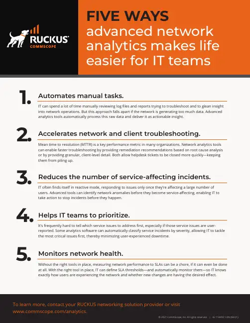
© 2020 CommScope, Inc. All rights reserved. | IG-114469-EN (04/20) © 2021 CommScope, Inc. All rights reserved. | IG-114492.1-EN (04/21) To learn more, contact your RUCKUS networking solution provider or visit /analytics.Automates manual tasks. 1.IT can spend a lot of time manually reviewing log files and reports trying to troubleshoot and to glean insight into network operations. But this approach falls apart if the network is generating too much data. Advanced analytics tools automatically process this raw data and deliver it as actionable insight.Mean time to resolution (MTTR) is a key performance metric in many organizations. Network analytics tools can enable faster troubleshooting by providing remediation recommendations based on root cause analysis or by providing granular, client-level detail. Both allow helpdesk tickets to be closed more quickly—keeping them from piling up. 2.Accelerates network and client troubleshooting. IT often finds itself in reactive mode, responding to issues only once they’re affecting a large number of users. Advanced tools can identify network anomalies before they become service-affecting, enabling IT to take action to stop incidents before they happen. Reduces the number of service-affecting incidents. 3.4.Helps IT teams to prioritize. It’s frequently hard to tell which service issues to address first, especially if those service issues are user-reported. Some analytics software can automatically classify service incidents by severity, allowing IT to tackle the most critical issues first, thereby minimizing user-experienced downtime .Monitors network health.5.Without the right tools in place, measuring network performance to SLAs can be a chore, if it can even be done at all. With the right tool in place, IT can define SLA thresholds—and automatically monitor them—so IT knows exactly how users are experiencing the network and whether new changes are having the desired effect.FIVE WAYS advanced network analytics makes life easier for IT teams。

磊科无线网卡用户手册Realtek 方案20101018v1.1.01商标、版权声明Copyright © 2010 深圳市磊科实业有限公司版权所有，保留所有权利未经深圳市磊科实业有限公司的许可，任何单位或个人不得以任何形式改编或转译部分或全部内容，不得以任何形式或任何方式（电子、机械、影音、录制或其他可能的方式）进行商品传播或用于任何商业、盈利目的。

®是深圳市磊科实业有限公司的注册商标。

本文档提及的其他所有商标和注册商标，由各自的所有人拥有。

本文档提供的资料，如有变更，恕不另行通知。

公司网站：全国免费支持电话：400-810-1616技术支持邮箱：fae-cd@公司地址：深圳市南山区高新技术产业园北区清华信息港B栋9楼邮编：518052A类设备声明此为A级产品，在生活环境中，该产品可能会造成无线电干扰，在这种情况下，可能需要用户对其干扰采取切实可行的保护措施。

包装清单包装盒里面应该有以下东西：●一片无线网卡。

●一张配置光盘C D。

●一本快速安装向导。

请确认包装盒里面有上述所有东西，如果有任何一个配件损坏或者丢失，请与你的经销商联系。

1.简介首先，感谢您选择磊科无线网卡，本手册将会详细说明磊科无线网卡硬件安装，客户端应用程序的基本功能。

1.1. 产品概述磊科无线网卡是功效强大的，可以快速、简便的安装到电脑上。

也可以用来在工作在点对点模式下，直接和其他卡连接以实现对等文件共享，或者在结构化模式下，同无线接入点或者路由器连接来进入办公室或者家里的网络里的I nternet。

磊科802. 11N 无线网卡基于标准的802.11n协议，兼容任何802.11g和802.11b 产品。

磊科802. 11G无线网卡基于标准的802.11g协议，兼容任何802.11b 产品。

注意：磊科无线网卡从接口方式来分，有两类：PCI/PCI-E和USB两大类，不同的型号，从速率来分，有54Mbps、150Mbps和300Mbps的网卡，可根据具体需求选择适当的网卡。

深圳城域网二期华为ME60业务配置指导书拟制:贾鹏日期：2007-2-2审核: 日期：审核: 日期：批准: 日期：修订记录日期修订版本描述作者2007-2-2 1.00初稿贾鹏1、全局配置华为ME60作为一个多业务网关可以做BAS使用，在实现方面与junipor ERX和Redback SE800不同，所有资源都是全局共享的，包括地址池，Radius组，路由表等等。

所以在配置业务的时候首先要配置一些共用的东西。

下面一一讲述。

1）配制loopback地址在全局配置模式下：Interface loopback 0Ip address 121.35.12.73 255.255.255.2552）配置Router id在全局配置模式下Router id 121.35.12.733）配置OSPF在全局配置模式下（以现网为例）：OspfArea XXXNetwork XXX.XXX.XXX.XXX 0.0.0.0Nssa4）配置ip pool在全局配置模式下（这里的顺序即为配置顺序）：Ip pool JT-ME60-Pool-01gateway 121.34.203.1 255.255.255.0section 0 121.34.203.2 121.34.203.254dns-server 202.96.128.68dns-server 202.96.134.133 secondary注意：这里的section代表一个地址范围，范围是0-7，也就是一个ip pool最多可以有8段地址。

当然这8段地址必须与gateway在同一网段。

5）配置Radius组在全局配置模式下：radius-server group gd_radiusradius-server authentication 61.140.4.144 1812 weight 0radius-server accounting 61.140.4.144 1813 weight 0radius-server shared-key szgnet^^注意：在配置Radius组中我们要配置发往Radius Server的IP地址，在这里我们一般选择Loopback地址作为认证地址。

网御星云安全网关PowerV 命令行操作手册VERSION 1.0明声♦本手册所含内容若有任何改动，恕不另行通知。

♦在法律法规的最大允许范围内，北京网御星云信息技术有限公司除就本手册和产品应负的瑕疵担保责任外，无论明示或默示，不作其它任何担保，包括（但不限于）本手册中推荐使用产品的适用性和安全性、产品的适销性和适合某特定用途的担保。

♦在法律法规的最大允许范围内，北京网御星云信息技术有限公司对于您的使用或不能使用本产品而发生的任何损坏（包括，但不限于直接或间接的个人损害、商业利润的损失、业务中断、商业信息的遗失或任何其它损失），不负任何赔偿责任。

♦本手册含受版权保护的信息，未经北京网御星云信息技术有限公司书面允许不得对本手册的任何部分进行影印、复制或翻译。

♦本手册使用于网御星云PowerV系列防火墙和VPN，在手册中称为安全网关。

文档少部分内容视产品具体型号略有不同，请以购买的实际产品为准。

♦网御星云不承担由于本资料中的任何不准确性引起的任何责任，网御星云保留不作另行通知的情况下对本资料进行变更、修改、转换或以其他方式修订的权利！北京网御星云信息技术有限公司号电8层中北京海淀中村南大街国区关6中信息大厦目 录目 录 (III)第1 章 前 言 (1)第2 章 命令行概述 (4)第3 章 快速入门 (25)第4 章 系统管理 (26)第5 章 网络管理 (76)第6 章 路由 (119)第7 章 防火墙 (135)第8 章 应用防护 (205)第9 章 用户认证 (287)第10 章 会话管理 (305)第11 章 VPN (308)第12 章 SSLVPN (327)第13 章 IPv6 (448)第14 章 漏洞扫描 (474)第15 章 状态监控 (477)第16 章 日志与报警 (480)第17 章 其他 (490)第1章 前 言1.1 导言员册该册绍过终《命令行操作手》是御册网安全网关Power V管理手中的一本。

网络协议配置向导了解用户界面网际操作系统(IOS)用户接口提供了几种不同的命令访问模式,每一个命令模式提供了一组相关的命令.为安全起见,IOS 提供了两种命令访问级别:User和Priviledged.无优先级的,用户模式称作User EXEC 模式,而Priviledged EXEC 被称作超级用户模式,需要有口令才能进入.用户模式下的命令集是超级用户下命令集的子集.在超级用户级别下,你可以进入配置模式和其下的十个特定的配置模式: interface, subinterface, controller, hub, map-list, map-class, line, router, ipx-router, router-map 等配置.大多数系统配置命令都有no 的形式,通常用no来取消掉一个配置过的命令.另外,在各种模式下的命令均可以用? 来查找自己所需的命令.下表列出几种命令模式,进入及退出的方法等等.* User EXEC 模式当用终端上路由器后,系统直接进入User EXEC模式,它的命令是超级用户下的子集.通常,User EXEC模式命令可以连接远端路由器,完成基本测试和系统信息显示.在User EXEC下的系统提示符是路由器名和后面紧跟的">"号:Router>在此下面,用户可以"?" 列出命令提示.*Priviledged EXEC 模式为安全起见,象UNIX操作系统一样,在路由器的指令系统中,设定了一个超级用户模式,在这个级别下,用户可以更改配置,监控网络状态等等.在User EXEC下,enable进入超级用户下.Router> enablePassword:Router#*Global 配置模式Global配置模式是在超级用户下实现的,它下面还有十个子模式,针对不同的配置方式.Router#configure terminalRouter(config)#*保存配置文件Cisco IOS 的指令系统是配置完后即时生效的,但当关掉电源后会自动丢失.因此,要想保留作的配置,必须在关机前把当前配置写入NVRAM中,下次开机时,自动从NVRAM中调入配置文件并执行.Router#write memory*监控程序在Global模式下,Cisco IOS作了许多监控程序,它可以帮助用户调试,监控网络状态,性能等等.Router# show ?在"?" 下有许多信息,帮助你找寻想要的命令.例如:Router# show conf 显示配置文件的配置Router# show running-config 显示当前正在运行的配置Router# show interface ethernet 0 查看以太口0的状态*slot/port在Cisco 7000/7500路由器上,不同的端口是在不同的接口卡上的.故指定某一个端口必须包括槽口号和端口号.例如:interface serial 4/5就表示串口卡在槽4上的第五个串口.配置IP这一章我们主要介绍怎样配置IP(Inetnet Protocol)协议.IP协议是目前应用最为普及的网络层协议,由于Internet的不断发展,TCP/IP协议也成为一种通用标准,并且在许多平台上,如各种Unix,Windows 95/NT, 在一系列IP相关的配置中,最基本和必需的是指定端口的IP地址,只有配了IP地址之后,才能使各个端口用IP协议与其它主机互相通信.∙指定一个网络接口的IP地址o指定一个端口的主IP 地址和网络掩码o在一个端口上指定多个IP 地址o在串口上指定IP处理∙地址解析协议o设置ARP打包o配主机名和IP地址OS/2,MVS,VM等大型机,小型机和微机的操作系统上均能支持.∙过滤IP包∙配置IP通过广域网∙监控和维护IP网络∙IP配置实例注意:以上的工作表并不是每一项都是必须的,请按照你的环境需要加以选择.指定一个网络接口的IP 地址一个IP标识了一个定位,使得IP数据包能被送出去.一些IP地址是预留的,它们不能作为主机,掩码或网络地址.表1列出了IP地址的范围,可以看出那些能被使用,那些是保留的.包括以下内容:∙指定一个端口的主IP 地址和网络掩码∙在一个端口上指定多个IP 地址∙在串口上指定IP处理表一: 预留的和有效的IP地址一个端口有一个主IP地址.指定一个端口的主IP 地址和网络掩码,在端口配置模式中完成:在一个端口上指定多个IP 地址通过软件可以支持多个IP地址在每一个端口上.你可以无限制的指定多个secondary地址, Secondary IP地址可以用在各种环境下.在端口配置模式下,指定多个地址:有关secondary IP 地址配置,请看"Creating a Network from Separates Subnets Example" 的举例说明.在串口上指定IP处理你可能希望在串口(serial)或者是作IP 隧道技术的端口上,不用指定一个IP地址而能在上面跑IP协议.这可以由IP unnumbered Address来实现.限制如下:∙串口使用HDLC,PPP,SLIP,LAPB,Frame Relay和tunnel interface打包方式.当串口用FR打包时,必须是点对点的.在X.25和SMDS打包时,不能用此特性.∙你不能用ping命令来探测端口是否是up,因为这个端口是没有IP地址的.简单网管协议(SNMP)远程监控端口状态.∙你不能通过unnumbered端口远程启动系统.∙在unnumbered端口上不支持IP安全选项.在端口配置模式下,实现unnumbered配置:在指定unnumbered 端口时,另外的那个端口不能也是unnumbered端口,并且这个端口必须是up的.(也就是说,该端口是工作正常的.)有关unnumbered IP 地址配置,请看"Serial Interfaces Configuration Example"的举例说明.地址解析协议一个设备在IP环境中有两种地址,一个是本身地址,也就是链路层地址(即MAC 地址),另一个是网络层地址(即IP地址).例如,以太网的设备互连,Cisco IOS软件首先要先确定48位的MAC地址.那么从IP地址到MAC地址的转换过程叫做地址解析(address resolution),而从MAC地址到IP地址的转换过程就叫反向地址解析(reverse address resolution).软件支持三种形式的地址解析: ARP,proxy ARP和Probe(类似ARP),反向地址解析: RARP.ARP,proxy ARP和RARP协议在RFC 826,1027和903分别作了定义,Probe是HP公司开发的用在IEEE-802.3网络中.设置ARP 打包默认的,在端口上是标准的以太网ARP打包方式.你可以根据你的网络需要改成SNAP或HP Probe方式.指定ARP打包方式,需完成:匹配主机名和IP 地址Cisco IOS 软件保持一张主机名和相应地址的表,叫做host name-to-address mapping.高层协议如Telnet,都是用主机名来标识设备的.因此,路由器和其它网络设备也需要了解它们.手工指定如下:配置IP 过滤表IP过滤表能够帮助控制网上包的传输.主要用在以下几个方面:∙控制一个端口的包传输∙控制虚拟终端访问数量∙限制路由更新的内容软件支持下面几种形式的IP过滤表:∙标准IP过滤表用源地址过滤∙扩展IP过滤表用源地址和目的地址过滤,并且可以过滤高层协议如Telnet,FTP等等.在Global配置模式下,定义标准的IP过滤表:标准的IP过滤表的表号1-99.在Global配置模式下,定义扩展的IP过滤表:扩展的IP过滤表的表号100-199.协议关键字有icmp,igmp,tcp,udp.在端口配置模式下,把某个IP过滤表加到端口上:有关IP过滤表配置,请看"IP Access List Configuration Example" 的举例说明.配置IP通过广域网你可以配置IP通过X.25,SMDS,Frame Relay和DDR网络.详细内容请参阅广域网配置向导.监控和维护IP 网络监控和维护你的网络,请完成以下工作:清除缓存,表单和数据库在EXEC模式下:显示系统和网络的状态在EXEC模式下:IP 配置实例∙Creat a Network from Separates Subnets Example ∙Serial Interface Configuration Example∙IP Access List Configuration Example∙标准IP过滤表配置实例∙限定虚拟终端访问实例∙扩展IP过滤表配置实例∙Ping Command ExampleCreat a Network from Separates Subnets Example在下面例子中,subnet 1和subnet 2被主干网分开.Configuration for Router Binterface ethernet 2ip address 192.5.10.1 255.255.255.0ip address 131.108.3.1 255.255.255.0 secondary Configuration for Router Cinterface ethernet 1ip address 192.5.10.2 255.255.255.0ip address 131.108.3.2 255.255.255.0 secondary Serial Interface Configuration Example在下面的例子中,把Ethernet 0的地址赋予Serial 1. Serial 1是unnumbered.interface ethernet 0ip address 145.22.4.67 255.255.255.0interface serial 1ip unnumbered ethernet 0IP Access List Configuration Example标准IP过滤表配置实例:该例表明在36.48.0.0这个网段上只允许B机(36.48.0.3)与A机通信,其它的36.0.0.0的网段如36.51.0.0可以与A机通信,而其它的如Internet用户均被过滤掉了.Configuration for Router Aaccess-list 2 permit 36.48.0.3access-list 2 deny 36.48.0.0 0.0.255.255access-list 2 permit 36.0.0.0 0.255.255.255!(Note:all other access denied)interface ethernet 0ip access-group 2 in限定虚拟终端访问实例:该例只允许在192.89.55.0这个网段上的主机访问路由器.Configuration for Routeraccess-list12 permit 192.89.55.0 0.0.0.255!line vty 0 4access-class 12 in扩展IP过滤表配置实例:该例允许内部网的所有主机都能登录上Internet,并且A机作smtp-server,B机作Web Server,C机作域名服务器,FTP服务器和邮件服务器.Configuration for Router!Allow existing TCP connectionaccess-list 105 permit tcp any any established!Allow ICMP messagesaccess-list 105 permit icmp any any!Allow SMTP to one hostaccess-list 105 permit tcp any host 201.236.15.14 eq smtp!Allow WWW to server (other services may be required)access-list 105 permit tcp any host 201.222.11.5 eq www!Allow DNS,FTP command and data,and smtpto another hostaccess-list 105 permit any host 201.222.11.7 eq domainaccess-list 105 permit any host 201.222.11.7 eq 42access-list 105 permit any host 201.222.11.7 eq ftpaccess-list 105 permit any host 201.222.11.7 eq ftp-dataaccess-list 105 permit any host 201.222.11.7 eq smtp!interface serial 0ip access-group 105 inPing Command Example在例子中,目的地址是131.108.1.111.源地址是131.108.105.62.Sandbox# pingProtocol [ip]:Target IP address: 131.108.1.111Repeat count [5]:10Datagram size [100]:64Timeout in seconds [2]:Extended commands [n]:Type escape sequence to abort.Sending 5, 100-byte ICMP Echos to 131.108.1.111, timeout is 2 seconds: !!!!!!!!!!Success rate is 100 percent, round-trip min/avg/max = 4/4/4 ms配置IP 路由协议这一章我们主要介绍怎样配置各种各样的IP(Internet IP)路由协议. IP路由协议分成两大类: 内部网关协议IGPs(Interior GatewayProtocols)和外部网关协议EGPs(ExteriorGateway Protocols). ∙选择路由协议的原则∙配置IGRPo Cisco's IGRP 的实现IGRP的路由交换o IGRP的配置∙配置Enhanced IGRPo Cisco's Enhanced IGRP的实现o EIGRP的配置o IGRP到EIGRP的迁移∙配置RIPo RIP的配置o RIP与IGRP,EIGRP的迁移∙配置静态路由∙IP路由协议的配置实例Cisco IOS支持的协议有:内部网关协议(它是在一个自治系统内部交换路由信息的路由协议)----- IGRP, EIGRP, OSPF, RIP 和IS-IS 等等.外部网关协议(它是为连接两个或多个自治系统的路由协议)----- BGP 和EGP等等.选择路由协议的原则选择一个路由协议是一个非常复杂的工作.当选择路由协议,参考以下几点:∙网络的大小和复杂性∙支持可变长掩码(VLSM).Enhanced IGRP,IS-IS,OSPF和静态路由支持可变长掩码∙网络流量大小∙安全需要∙网络延迟特性下面就分别介绍各种路由协议的特点和配置.配置IGRP内部网关路由协议(Interior Gateway Routing Protocol---- IGRP)是一个动态的,长跨度的路由协议,它是Cisco 公司八十年代中期设计实现的,在一个自治系统内具有高跨度,适合复杂网络的特点.Cisco's IGRP的实现IGRP的网络延迟,带宽,可靠性和负载都是可由用户配置决定的.IGRP广播三种类型的路由:内部的,系统的和外部的.如图所示.内部的路由是在一台路由器的端口上连接子网的路由.如果一台路由器连接的网络是非子网的,IGRP就不广播内部路由.图 1 :内部,系统和外部路由系统路由是一个自治系统内的路由.Cisco IOS 软件从直连的网络接口上获得系统路由,并把它提供给其它的支持IGRP协议的路由器或访问服务器.系统路由不包括子网信息.外部路由是自治系统之间的路由.IGRP的路由交换默认的,一个运行IGRP路由协议的路由器每90秒广播一次路由信息.如果在270秒内未收到某路由器的回应,它则认为目前该路由器不可到达;若在630秒后仍未有应答,则把有关它的路由信息从路由表中删掉.IGRP的配置指定路由器IGRP协议:请参阅"Configure IGRP Example",更加详细的资料请看Cisco CD 或Cisco的主页.配置Enhanced IGRPEnhanced IGRP是Cisco公司开发的IGRP的增强的版本.它使用与IGRP相同的路由算法,但它在许多方面对IGRP作了较大的改进.Cisco's Enhanced IGRP的实现Cisco's Enhanced IGRP提供了以下特性:∙自动重新分配-----IP IGRP路由可以自动的重新分配到EIGRP中,IP EIGRP也可以自动的重新分配到IGRP中.如果愿意,也可以关掉重新分配.∙可扩展的网络-----对于IP RIP,你的网络最大只有15个hops,而当使用EIGRP时,最大可以有224个hops.∙触发的路由表-----EIGRP并不象IGRP那样经过一定的时间间隔后交换路由信息的,而是只有当路由表有变化时才把路由表广播出去的,叫做触发式的(triggered).∙支持可变长掩码(VLSM)配置Enhanced IGRP指定EIGRP路由协议:更加详细的资料请看Cisco CD 或Cisco的主页.IGRP到EIGRP的迁移在同一个自治系统的IGRP和EIGRP是自动能够重新分配的,而在不同两个自治系统之间,作如下配置:请参阅"IGRP and EIGRP Redistribution Example",更加详细的资料请看Cisco CD 或Cisco的主页.配置RIP路由信息协议(Routing Information Protocol ---RIP)是一个相对比较老的,但仍被广泛使用的路由协议.RIP广播一个UDP数据包更换路由信息,每个路由器间隔30秒更换一次路由信息,在180秒内未收到某路由器的回应,它则认为目前该路由器不可到达;若在270秒后仍未有应答,则把有关它的路由信息从路由表中删掉.RIP的配置指定IP RIP路由协议:RIP到IGRP,EIGRP的迁移请参阅"RIP and EIGRP Redistribution Example",更加详细的资料请看Cisco CD 或Cisco的主页.配置静态路由在某些环境下,我们需要尽量小的路由交换和其它一些特殊环境下会用到静态路由.请参阅"Static Routing Redistribution Configure Example".IP路由协议实例配置∙Configure IGRP Example∙IGRP and EIGRP Redistribution Example∙RIP and EIGRP Redistribution Example∙Static Routing Redistribution Configure Example∙Route Filtering Example∙Redistribution FilteringConfigure IGRP Example假设RouterA连接到130.108.0.0和10.0.0.0这两个直连网段上.RouterA#config terminal (在"#"提示符下)RouterA(config)#router igrp 15 (进入配置模式)RouterA(config-router)#network 130.108.0.0 (进入路由配置子模式)RouterA(config-router)#network 10.0.0.0IGRP and EIGRP Redistribution Example在AS 200和AS 100两个自治系统内,分别跑EIGRP和IGRP协议,要想互相通信:Configuration for RouterArouter eigrp 200network 201.222.5.0redistribute igrp 100default-mertic 56 2000 255 1 1500router igrp 100network 131.108.0.0redistribute eigrp 200default-metric 56 2000 255 1 1500RIP and EIGRP Redistribution ExampleConfiguration for RouterArouter ripnetwork 201.222.5.0redistribute eigrp 100default-mertic 3router eigrp 100network 131.108.0.0redistribute ripdefault-metric 56 2000 255 1 1500Static Routing Redistribution Configure Example Configuration for RouterAip route 131.108.1.0 255.255.255.0 131.108.2.1!router eigrp 1network 192.31.7.0default-metric 10000 100 255 1 1500redistribute staticdistribute-list 3 out static!access-list 3 permit 131.108.0.0 0.0.255.255 Route Filtering Example在路由器B上,过滤掉由10.0.0.0发送过来的路由信息,那么在201.222.5.0这个网段上是不能与10.0.0.0这个网通信的.换句话说,在201.222.5.0一端隐藏了10.0.0.0这个网.Configuration for Routerrouter eigrp 1network 131.108.0.0network 201.222.5.0distribute-list 7 out s0!access-list 7 permit 131.108.0.0 0.0.255.255access-list 7 deny 10.0.0.0 0.255.255.255Redistribution Filtering效果同上,但是在两个不同的路由协议下的.Configuration for Routerrouter ripnetwork 201.222.5.0redistribute eigrp 100default-mertic 3!router eigrp 100network 131.108.0.0redistribute ripdefault-metric 56 2000 255 1 1500distribute-list 7 out rip!access-list 7 deny 10.0.0.0 0.255.255.255 access-lsit 7 permit 0.0.0.0 255.255.255.255。

HeadquartersSales 5453 Great Amer i ca Parkway Santa Clara, CA 95054 USA+ 1 408 547-5500+1408547-5501+ 1 866 Support +1408547-5502+ 1866 4 76-0000support-w ******************************© Copyright 2019 A rista Networks , Inc. The information contained here i n is subject to change without notice. Arista Networks and the Arista logo are trademarks of Arista Networks, Inc in the United States and other countries. Other product or serv i ce names may be trademarks or service marks of others .ContentsChapter 1. About This Guide (3)Chapter 2. Package Content (4)Chapter 3. C-110 Overview (5)Front Panel of C-110 (5)Rear Panel of C-110 (5)Chapter 4. Install the C-110 (7)Connect the C-110 to the Network (7)Connect the C-110 using PoE (8)Mount the C-110 (8)Power On the C-110 (9)Using the C-100 with Power Adapter (9)Chapter 5. C-110 Troubleshooting (10)Chapter 6. Appendix A: AP-Server Mutual Authentication (11)Chapter 1. About This GuideThis installation guide explains how to deploy the C-110 access point (AP).Important: Please read the EULA before installing C-110. You can download and read the EULA from https:// /en/support/product-documentation.Installing the AP constitutes your acceptance of the terms and conditions of the EULA mentioned above in this document.Intended AudienceThis guide can be referred by anyone who wants to install and configure the C-110 access point.Document OverviewThis guide contains the following chapters:•Package Content (page 4)•C-110 Overview (page 5)•Installing the C-110 (page 7)•C-110 Troubleshooting (page 10)Note: All instances of the term 'server' in this document refer to the Wireless Manager, unless the server name or type is explicitly stated.Product and Documentation UpdatesTo receive important news on product updates, please visit our website at https:///en/support/product-documentation. We continuously enhance our product documentation based on customer feedbackChapter 2. Package ContentThe C-110 package must contain the components shown in the figure below.Figure 1: C-110 Package ComponentsImportant: The MAC address of the device is printed on a label at the bottom of the product and the packaging box. Note down the MAC address, before mounting the device on the ceiling or at a location that is difficult to access. If the package is not complete, please contact the Arista Networks Technical Support Team at ***********************, or return the package to the vendor or dealer where you purchased the product.Chapter 3. C-110 OverviewC-110 is a 2x2 802.11a/b/g/n/ac access point.This chapter provides an overview of the C-110 and describes:•The Front Panel of the C-110 (page 5).•The Rear Panel of the C-110 (page 5).Front Panel of C-110The front panel of the C-110 has 5 functional LEDs that indicate the working of the device.Figure 2: C-110 Front Panel LEDsThe following table indicates the device states based on the LEDs.Table 1: C-110 LED Status DescriptionLED Status DescriptionPowerSolid Green Power ONOFF Power OFF5 GHzSolid Green No activity on 5 GHz radioBlinking Green Wireless activity on 5 GHz radio2.4 GHzSolid Green No activity on 2.4 GHz radioBlinking Green Wireless activity on 2.4 GHz radioRadio 3Blinking Green Activity on third radioLAN1/2Solid Green Wired Extension/VLAN Extension enabledRear Panel of C-110The rear panel of the C-110 provides an PoE Ethernet port that enables you to connect the device to a wired LAN through a switch or a hub and power the device by using the 802.3af standard.C-110 | 3 - C-110 Overview | 6Figure 3: C-110 Rear PanelPortDescription Connector Type Speed/Protocol Ethernet (LAN1/PoE)Gigabit Ethernet port used to connect to the wired LAN and communicate with the Arista cloud or server. This port can also be used to power the device using the 802.3af Power over Ethernet (PoE) standard.RJ45•10/100/1000 Mbps Gigabit Ethernet •802.3af Class 0 PoE •PoE input voltage: 48V Ethernet (LAN2)Gigabit Ethernet port that can be used for wired extension for an SSID.RJ4510/100/1000 Mbps Gigabit Ethernet Reset Pin HoleReset to factory default settings. To reset the device, press and hold the Reset Pin Hole for 10 sec until all LEDs go off which indicates that the device has rebooted. Pressing the Reset Pin Hole while the device is booting up will not have any effect.You should perform this operation only when the device is running.Pin hole push button Hold down and power cycle the device to reset DC IN Enables you to connect to and power on device using 12 V DC power with1.5 ampere. 6.3 mm barrel--When you reset the device, the following settings are reset:•Config shell password is reset to config .•Server discovery value is erased and changed to the default, (primary) and wifi-security-server (secondary).•All the VLAN configurations are lost.•If static IP is configured on the device, the IP address is erased and DHCP mode is set. The factory default IP address ofthe device is 169.254.11.74.Chapter 4. Install the C-110This chapter contains the stepwise procedure to install the C-110 device.Zero-Configuration of C-110 as Access PointZero-configuration is supported under the following conditions:•The device is in AP mode with background scanning on and no SSID configured.• A DNS entry wifi-security-server is set up on all the DNS servers. This entry should point to the IP address of the server.By default, the device looks for the DNS entry wifi-security-server.•The device is placed on a subnet that is DHCP enabled.Important: If the device is placed on a network segment that is separated from the server by a firewall, you must first open port 3851 for User Datagram Protocol (UDP) and Transport Control Protocol (TCP) bidirectional traffic on that firewall. This port number is assigned to Arista Networks. If multiple devices are set up to connect to multiple servers, zero-configuration is not possible. In this case, you must manually configure the APs. See the Access Point Configuration Guide on our website at https:///en/support/product-documentation .Take a configured C-110, that is, ensure that a static IP is assigned to the device or the settings have been changed for DHCP. Note down the MAC address and the IP address of the device in a safe place before it is installed in a hard-to-reach location. The MAC address of the device is printed on a label at the bottom of the product.The steps to install the device with no configuration (zero-configuration) are as follows:1.Mount the device. (page 8)2.Power On the device. (page 9)3.Connect device to the network. (page 7)Connect the C-110 to the NetworkTo connect C-110 to the network, perform the following steps:1.Ensure that a DHCP server is available on the network to enable network configuration of the C-110.2.Add the DNS entry wifi-security-server on all DNS servers. This entry should point to the IP address of the server.3.Ensure that DHCP is running on the subnet to which the device will be connected.4.Check the status LEDs on the device. If all LEDs glow green, then the device is operational and connected to the server.5.Log on to the server using ssh and run the get sensor list command.You will see a list of all Arista devices that are recognized by the server. Single Sign-On users can go to the Devices tab in Wireless Manager and check whether the device is visible under the Devices tab.The device is connected and ready to go operational.Note: If the zero configuration is not successful, the device must be configured manually.Important: If DHCP is not enabled on a subnet, the device cannot connect to that subnet with zero-configuration. If the DNS entry is not present on the DNS servers or if you do not have the DHCP serverrunning on the subnet, you must manually configure the device. See the Access Point Configuration guide onour website at https:///en/support/product-documentation .C-110 | 4 - Install the C-110 | 8Connect the C-110 using PoEIf you are using a PoE injector, make sure the data connection is plugged into a suitable switch port with proper network connectivity.Mount the C-110The C-110 mounting procedure can be divided into two parts:1.Affix the bracket to the T -grid: Use the mounting bracket to install the C-110 on the ceiling. Fix the bracket to the T-grid and rotate the bracket so that it snaps on the T-grid. The bracket is now parallel to an arm of the T-grid. Ensure that the bracket is properly snapped to the T-grid. Refer to the images given below.2.Mounting C-110 on the bracket: Place the first mounting post on the rear-side of the device on to the lower notch of thebracket. Rotate the device such that the center mounting post fits in to the center notch on the bracket. Ensure that all the mounting posts on the rear-side of the device are snapped in to the respective notches on the bracket. The mounting posts on the rear-side of the device are now properly fit in the respective notches of the bracket and device is mounted properly.Mounting Instructions using the Silhouette/Interlude Bracket Mount: The Silhouette/Interlude mounting bracket is not a part of the standard package and must be procured separately. The mounting instructions for the Silhouette/ Interlude Bracket Mount are similar to the Standard Package Content's mounting instructions.C-110 | 4 - Install the C-110 | 9 Note: You should label the devices using MAC addresses or at least your own convention. For example, use serial numbers, so that you can easily identify the devices.Power On the C-110The C-110 device can be powered on by plugging one end of the Ethernet cable into the PoE (802.3af) switch or injector andthe other end into the Ethernet/PoE port on the C-110. Ensure the PoE source you are using is turned ON.As an alternative to PoE, you can insert a compatible power adaptor plug into an AC power outlet and the other end into the power input port on the C-110.Note: If you are not using PoE, ensure that you use only an AC power adaptor supported by the C-110 access point (AP).Using the C-100 with Power AdapterTo power up the device with power adapter, perform the following steps:1.Plug the power cable into the DC power receptacle at the rear of the device.2.Plug the other end of the power cable into an 110V~240V 50/60 Hz AC power source.3.Wait until the device is ready. Refer to the LED details table.Chapter 5. C-110 TroubleshootingThe table below lists some of the troubleshooting guidelines for C-110.Diagnosis SolutionThe device did not receive a valid IP address via the DHCP.Ensure that the DHCP server is on and available on the VLAN/subnetto which the device is connected. If the device still fails to get a valid IPaddress, you can reboot it to see if the problem is resolved.The Ethernet cable is loose. The device is probably disconnected from theEnsure that the Ethernet cable is connected.network.Unable to connect to the server Ensure that the server is running and is reachable from the network to whichthe device is attached. If there is a firewall or a router with ACLs enabledbetween the device and the server, ensure that the traffic is allowed onUDP port 3851. Use the server IP-based discovery and ensure that youhave correctly entered the DNS name, wifi-security-server , on the DNSserver. Also, ensure that the DNS server IP addresses are either correctlyconfigured on the, or are provided by the DHCP server. It is also possiblethat the AP is unable to connect to the server because it has failed toauthenticate with the server. In this case, an 'Authentication failed for ' eventis raised on the server. Refer to the event for recommended action.The AP has encountered a problem.If you are using Arista Cloud Services, then open the TCP port 443 (SSL).If you have an on-premises installation, then open the ports UDP 3851 andport 80. If you are using a Proxy, Web Accelerator or URL Content Filter inbetween the AP and the Internet, ensure the settings allow communicationbetween the AP and Arista Cloud Services. If your configuration requiresyou to specify an exact IP address or IP range for Arista Cloud Services,************************************.Chapter 6. Appendix A: AP-Server Mutual AuthenticationThe AP-server communication begins with a mutual authentication step in which the AP and server authenticate each other using a shared secret. The AP-server communication takes place only if this authentication succeeds.After the authentication succeeds, a session key is generated. All communication between the AP and server from this point on is encrypted using the session key.The AP and server are shipped with the same default value of the shared secret. The CLI commands are provided on both server and AP for changing the shared secret.Note: After the shared secret (communication key) is changed on the server, all APs connected to the server will automatically be set up to use the new communication key. APs that are not connected to the server at this time must be manually set up with the same communication key to enable communication with this server.Note: Although the server is backward compatible, that is, older version APs can connect to a newer version server, this is not recommended.。