Three-parameter AVO inversion with PP and PS data using offset binning
- 格式:pdf
- 大小:743.72 KB
- 文档页数:22

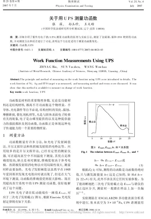
第25卷第4期2007年7月物理测试P hysics Examination and T estingV ol.25,No.4July 2007作者简介:张 滨(1978),女,硕士生; E -mail:b inzhang@ ; 修订日期:2006-11-14关于用U PS 测量功函数张 滨, 孙玉珍, 王文皓(中国科学院金属研究所分析测试部,辽宁沈阳110016)摘 要:详细介绍了紫外光电子谱(U P S)测量功函数的原理与实验方法,测量了金属镍、银和IT O 靶材的功函数,并对测量方法和误差进行了讨论,表明这个方法更适用于测量功函数变化。
关键词:功函数;U P S中图分类号:O433.1 文献标识码:A 文章编号:1001-0777(2007)04-0021-03Work Function Measurements Using UPSZH NA G Bin, SU N Yu -zhen, WANG Wen -hao(Institut e o f M etal R esear ch,Chinese A cademy o f Sciences,Sheny ang 110016,L iaoning ,China)Abstract:T he pr inciple and method of measur ing o n the w ork funct ion using U PS w ere intr oduced in details.T he w or k funct ion of N i,A g and IT O tar get w as measured,and measuring method and er ror s w ere discussed.It was show that this metho d is av ailable t o measur e on change o f wo rk functio n.Key words:w ork function;U P S功函数是材料的重要物理参数,无论是功能材料还是结构材料,都离不开功函数这个物理量。


Trans. Nonferrous Met. Soc. China 22(2012) 1064í1072Correlation between welding and hardening parameters offriction stir welded joints of 2017 aluminum alloyHassen BOUZAIENE, Mohamed-Ali REZGUI, Mahfoudh AYADI, Ali ZGHALResearch Unit in Solid Mechanics, Structures and Technological Development (99-UR11-46),Higher School of Sciences and Techniques of Tunis, TunisiaReceived 7 September 2011; accepted 1 January 2011Abstract: An experimental study was undertaken to express the hardening Swift law according to friction stir welding (FSW) aluminum alloy 2017. Tensile tests of welded joints were run in accordance with face centered composite design. Two types of identified models based on least square method and response surface method were used to assess the contribution of FSW independent factors on the hardening parameters. These models were introduced into finite-element code “Abaqus” to simulate tensile tests of welded joints. The relative average deviation criterion, between the experimental data and the numerical simulations of tension-elongation of tensile tests, shows good agreement between the experimental results and the predicted hardening models. These results can be used to perform multi-criteria optimization for carrying out specific welds or conducting numerical simulation of plastic deformation of forming process of FSW parts such as hydroforming, bending and forging.Key words: friction stir welding; response surface methodology; face centered central composite design; hardening; simulation; relative average deviation criterion1 IntroductionFriction stir welding (FSW) is initially invented and patented at the Welding Institute, Cambridge, United Kingdom (TWI) in 1991 [1] to improve welded joint quality of aluminum alloys. FSW is a solid state joining process which was therefore developed systematically for material difficult to weld and then extended to dissimilar material welding [2], and underwater welding [3]. It is a continuous and autogenously process. It makes use of a rotating tool pin moving along the joint interface and a tool shoulder applying a severe plastic deformation [4].The process is completely mechanical, therefore welding operation and weld energy are accurately controlled. B asing on the same welding parameters, welding joint quality is similar from a weld to another.Approximate models show that FSW could be successfully modeled as a forging and extrusion process [5]. The plastic deformation field in FSW is compared with that in metal cutting [6í8]. The predominant deformation during FSW, particularly in vicinities of thetool, is expected to be simple shear, and parallel to the tool surface [9]. When the workpiece material sticks to the tool, heat is generated at the tool/workpiece contact due to shear deformation. The material becomes in paste state favoring the stirring process within the thermomechanically affected zone, causing a large plastic deformation which alters micro and macro structure and changes properties in polycrystalline materials [10].The development of the mechanical behavior model, of heterogeneous structure of the welded zone, is based on a composite material approach, therefore it must takes into account material properties associated with the different welded regions [11]. The global mechanical behavior of FSW joint was studied through the measurement of stress strain performed in transverse [12,13] and longitudinal [14] directions compared with the weld direction. Finite element models were also developed to study the flow patterns and the residual stresses in FSW [15]. B ased on all these models, numerical simulations were performed in order to investigate the effects of welding parameters and tool geometry on welded material behaviors [16] to predict the feasibility of the process on various shape parts [17].Corresponding author: Mohamed-Ali REZGUI; E-mail: mohamedali.rezgui@ DOI: 10.1016/S1003-6326(11)61284-3Hassen BOUZAIENE, et al/Trans. Nonferrous Met. Soc. China 22(2012) 1064í1072 1065 However, the majority of optimization studies of theFSW process were carried out without being connectedto FSW parameters.In the present study, from experimental andmodeling standpoint, the mechanical behavior of FSWaluminum alloy 2017 was examined by performingtensile tests in longitudinal direction compared with theweld direction. It is a matter of identifying the materialparameters of Swift hardening law [18] according to theFSW parameters, so mechanical properties could bepredicted and optimized under FSW operating conditions.The strategy carried out rests on the response surfacemethod (RSM) involving a face centered centralcomposite design to fit an empirical models of materialparameters of Swift hardening law. RSM is a collectionof mathematical and statistical technique, useful formodeling and analysis problems in which response ofinterest is influenced by several variables; its objective isto optimize this response [19]. The diagnostic checkingtests provided by the analysis of variance (ANOV A) suchas sequential F-test, Lack-of-Fit (LoF) test, coefficient ofdetermination (R2), adjusted coefficient of determination(2adjR) are used to select the adequacy models [20].2 Experimental2.1 Welding processThe aluminum alloy 2017 chosen for investigationhas good mechanical characteristics (Table 1), excellentmachinability and formability, and is mostly used ingeneral mechanics applications from high strengthsuitable for heavy-duty structural parts.Table 1 Mechanical properties of aluminum alloy 2017Ultimate tensile strength/MPaYieldstrength/MPaElongation/%Vickershardness427 276 22 118 The experimental set up used in this study was designed in Kef Institute of Technology (Tunisia). A 7.5 kW powered universal mill (Momac model) with 5 to 1700 r/min and welding feed rate ranging from 16 to 1080 mm/min was used. Aluminum alloy 2017 plate of6 mm in thickness was cut and machined into rectangular welding samples of 250 mm×90 mm. Welding test was performed using two samples in butt-configuration, in contact along their larger edge, fixed on a metal frame which was clamped on the machine milling table.To ensure the repeatability of the FSW process, clamping torque and flatness surface of the plates to be welded are controlled for each welding test. At the end of welding operation, around 80 s are respected before the withdrawal of the tool and the extracting of the welded parts. In this experimental study, we purpose to screen theeffects of three operating factors, i.e. tool rotational speed N, tool welding feed F and diameter ratio r, on hardening parameters from Swift’s hardening law such as strength coefficient (k), initial yield strain (İ0) and hardening exponent (n). The ratio (r=d/D) of pin diameter (d) to shoulder diameter (D), is intended to optimize the tool geometry [21í23]. The welding tool is manufactured from a high alloy steel (Fig. 1).Fig. 1 FSW tool geometry (mm)Preliminary welding tests were performed to identify both higher and lower levels of each considered factors. These limits are fixed from visual inspections of the external morphology and cross sections of the welded joints with no macroscopic defects such as surface irregularities, excessive flash, and lack of penetration or surface-open tunnels. However, among these limits one is not sure to have a safe welded joint so often, but they show great potential on defect avoidance. Figure 2 shows some external macroscopic defects observed beyond the limit levels established for each factor. Table 2 lists the processing factors as well as levels assigned to each, and Table 3 shows the fixed levels for other factors needed to success the welding tests.A face centered central composite design, which comes under the RSM approach, with three factors was used to characterize the nature of the welded joints by determining hardening parameters. In this design the star points are at the center of each face of the factorial space (Į=±1), all factors are run at three levels, which are í1, 0, +1 in term of the coded values (Table 4). The experiment plan has been run in random way to avoid systematic errors.2.2 Tensile testsThe tensile tests are performed on a Testometric’s universal testing machines FSí300 kN. The tensile test specimens (ASME E8Mí04) proposed for characterizing the mechanical behavior of the FSW joint, were cut inHassen BOUZAIENE, et al/Trans. Nonferrous Met. Soc. China 22(2012) 1064í10721066Fig. 2 Types of macroscopic defectsTable 2 Levels for operating parameters for FSW processFactorLow level (í1) Center point (0) High level(+1)N /(r·min í1) 653 910 1280 F /(mm·min í1)67 86 109r /%33 39 44Table 3 Welding parametersPin height/ mm Shoulder diameter/ mm Small diameter pin/mm Tool’s inclination angle/(°) Penetrationdepth of shoulder/mm5.3 18 4 30.78longitudinal direction compared with the weld direction, so that active zone is enclosed in the central weld zone (Fig. 3). Figure 4 shows the tensile specimens after fracture.Ultimately, it is a matter of experimental evaluation of hardening parameters of the behavior of FSW joints (k , İ0, n ) according to Swift’s hardening law:n k )(p 0H H V (1)These parameters are required to identify the plastic deformation aptitude of the FSW joints. They are also needed for numerical simulations of forming operations on welded plates. The hardening parameters have been calculated by least square method (LSM) from the stressüstrain curves data. Table 4 shows the experimental design as well as dataset performance characteristics according to the FSW parameters of aluminum Alloy 2017.3 Experimental results3.1 Development of mathematical modelsAlthough the basic principles of FSW are very simple, it involves complex phenomena related to thermo-mechanical and metallurgical transformation that causes strong microstructural heterogeneities in the welded zone. From an energy standpoint, welding process is generated by converting mechanical energy provided by FSW tool into other types of energy such as heat, plastic deformation and microstructural transformations. The nonlinear character of these different dissipation forms can justify research for nonlinear prediction models whose accuracy generally depends on the order of the models relating the responses to welding parameters. For this reason, we chose the RSM which is helpful in developing a suitable approximation for the true functional relationships between quantitative factors (x 1, x 2, Ă, x k ) and the response surface or response functions Y (k , İ0, n ) that may characterize the nature of the welded joints as follows:r 21),,,(e x x x f Y k (2)Hassen BOUZAIENE, et al/Trans. Nonferrous Met. Soc. China 22(2012) 1064í10721067Table 4 Face centered central composite design for FSW of aluminum alloy 2017Factors levelCoded Actual Hardening parameterTypeStandard orderN F r N /(r·m í1)F /(mm·min í1)r /% k /MPan İ0/%1 í1 í1 í165367 33629.7 0.3296 0.00202 1 í1 í1 1280 67 33 654.7 0.4514 0.0035 3 í1 1 í1 653109 33 587.8 0.3712 0.0025 4 1 1 í1 1280 109 33 689.2 0.4856 0.00555 í1 í1 1 653 67 44 642.3 0.4524 0.00256 1 í1 1128067 44 218.6 0.2447 0.0015 7 í1 1 1 653 109 44 685.5 0.4885 0.0035 Factorialdesign8 1 1 1 1280 109 44 332.5 0.3405 0.00209 0 0 0 91086 39 624.9 0.4257 0.0025 10 0 0 0 910 86 39 639.9 0.4292 0.0025 11 0 0 0 910 86 39 640.9 0.4011 0.0020 Center point12 0 0 0 910 86 39 598.6 0.3960 0.0023 13 í1 0 0 653 86 39 690.6 0.4748 0.0027 14 1 0 0 128086 39 505.6 0.3909 0.0030 15 0 í1 091067 39499 0.3317 0.001716 0 1 0 910 109 39 545.6 0.4157 0.0026 17 0 0 í1 910 86 33 672.1 0.4385 0.0027 Star point18 0 019108644 509.7 0.41750.0019Fig. 3 Tensile test specimens (ASME E8Mí04) cut in longitudinal direction compared with weld direction (mm)Fig. 4 Tensile specimens after fractureThe residual error term (e r ) measures theexperimental errors. Such relationship was developed as quadratic polynomial under multiple regression form [19,20]:¦¦¦ r 20e x x b x b x b b Y j i ij i ii i i (3)where b 0 is an intercept or the average of response; b i , b ii , and b ij represent regression coefficients. For the three factors, the selected polynomial could be expressed as:2332222113210r b F b N b r b F b N b b YFr b Nr b NF b 231312 (4)In applying the RSM, the independent variable Y was viewed as surface to which a mathematical model was fitted. The adequacy of the developed model was tested using the analysis of variance (ANOV A) which quantifies the amount of variation in a process and determines if it is significant or is caused by random noise.3.2 Mathematic model of hardening parametersTable 5 lists the coefficients of the best linear regression models. All selected parameters (N , F , r ) for k and İ0 are statistically significant (P-value less than 0.05) at the 95% confidence level. However, for the response n , the term b 3r having a P-value=0.0654>0.05 is not statistically significant at the 95% confidence level even though the term b 13Nr is statistically significant. Consequently, b 3(r ) is kept in the model to improve the Lack-of-Fit test (Table 6). Furthermore, only theHassen BOUZAIENE, et al/Trans. Nonferrous Met. Soc. China 22(2012) 1064í10721068Table 5 Coefficients of regression models for hardening parametersStrength coefficient (k) Hardeningcoefficient(n) Initial yield strain (İ0) CoefficientEst. SEP-value Est SE P-valueEst/10í4 SE/10í4 P-value b0 610.39,48<10í4 0.422 0.0073 <10-4 22.8 1.010 <10-4 b1 í83.58.48<10í4 í0.020 0.0065 0.0091 2.30 0.912 0.0267 b2 19.68.480.0410.0290.00650.00084.900.9120.0002b3 í84.58.48<10í4 í0.013 0.0065 0.0654 í4.80 0.912 0.0002 b11 5.561.3670.0009b22 í61.812.720.0005í0.0310.00980.009b33b12b13 í112.99.48<10í4 í0.074 0.0073 <10-4 -8,75 1.010 <10-4 b23R2 95.90% 92.38% 92.84%2adjR 94.19% 89.21% 89.86% SE of est. 30.7 0.021 2.9×10í4Est: Estimate; SE: Standard Error; SE of est.: Standard error of estimateTable 6 ANOV A for hardening parametersk n İ0Source of variationSS Df P-Value SS Df P-Value SS/10í7 Df P-Value Model 263946.0 5 <10í4 0.062357 5 <10í4 129.324 5 <10í4Residual 11296.4 12 0.005140912 9.97 12Lack-of-Fit 10130.4 9 0.2065 0.00428669 0.3678 8.295 9 0.3723 Pure error 1166.07 3 0.0008543 3 1.675 3 Total correction 275243.017 0.06749817 139.294 17 DW-value 1.31 1.42 2.26DW: Durbin-Watson statistic; SS: Sum of squares; D f: Degree of freedominteraction (Nír) is statistically significant on the three responses (Fig. 5). According to the adjusted R2 statistic, the selected models explain 94.19%, 89.21% and 89.86% of the variability in k, n and İ0 respectively.The ANOV A (Table 6) for the hardening parameter shows that all models (k, n, İ0) represent statistically significant relationships between the variables in each model at the 99% confidence level (P-value<10í4). The Lack-of-Fit test confirms that these models (k, n, İ0) are adequate to describe the observed data (P-value>0.05) at the 95% confidence level. The DW statistic test indicates that there is probably not any serious autocorrelation in their residuals (DW-value>1.4). The normal probability plots of the residuals suggest that the error terms, for these models, are indeed normally distributed (Fig. 6). The response surface models in terms of coded variables (Eqs. (5)í(7)) are shown in Fig. 7.k=610.3–83.5 N+19.6 F–84.5 r –61.8 F2–112.9 Nr(5) n=0.422–0.020 N+0.029 F–0.013 r–0.031 F2–0.074 Nr(6) İ0=22.8+2.3 N+4.90 F–4.80 r+5.56 N2–8.75 Nr(7) Fig. 5 Interaction plots of Nír (rotational speedídiameter ratio): (a) Strength coefficient k; (b) Hardening coefficient n;(c) Initial yield strain İ0Hassen BOUZAIENE, et al/Trans. Nonferrous Met. Soc. China 22(2012) 1064í1072 1069Fig. 6 Normal probability plots for residual: (a) Strength coefficient k; (b) Hardening coefficient n; (c) Initial yield strain İ04 Validation of identified modelsValidation tests of the identified models were performed through comparative study between the experimental models (EM) of tensile tests and the computed responses given by numerical simulations of the same tests (Fig. 8). The computed responses, expressed in the form of tension and elongation, wereFig. 7 Response surfaces plots: (a) Strength coefficient k;(b) Hardening coefficient n; (c) Initial yield strain İ0 established by examining welded joints having an elastoplastic behavior in accordance with the Swift hardening law (Eq. (1)). These computed responses were deduced from the numerical simulations using the finite element code Abaqus/Implicit, in which the introduced elastoplastic behavior was obtained from the least square hardening models (LSHM) (Table 4) and the response surface hardening models (RSHM) (Table 5). The highest deviations (<10%), between EM and computed response, were recorded with the RSHM. Increasing deviations, as shown in Fig. 8, is due to the effect of combining damage with plastic strains accumulatedHassen BOUZAIENE, et al/Trans. Nonferrous Met. Soc. China 22(2012) 1064í10721070Fig. 8 Relationship between tension and elongation: Confrontation between experimental model (EM), and computed responses (LSHM, RSHM) for three experimental testsduring the onset of localized necking.The relative average deviation criterion (EM/LSHM ]) between the experimental data and the numerical predictions of tensions, was used to assess the quality of the identified models.¦¸¸¹·¨¨©§'' '2exp num exp exp/num )()()(1i i i L F L F L F N] (8)where N is the number of experimental measurements,F exp (ǻL i ) and F num (ǻL i ) are respectively the experimental and predicated tensions relating to the i-th elongation ǻL i . Figure 9 illustrates that the relative average deviation of EM/LSHM (EM/LSHM ]) ranges between 1.64% and 6.75% while the relative average deviation of EM/RSHM (EM/RSHM ]) ranges between 4.52% and 9.32%.Fig. 9 Distribution of relative average deviations for most representative experimental testsFor the deviation within limits fluctuating between 4.52% and 6.75% the estimated models (LSHM and RSHM) are comparable. This applies particularly to welded joints characterized by a strength coefficient (k ), ranging from 520 to 610 MPa and a hardening exponent (n ) ranging between 0.30 and 0.45.5 DiscussionIn this study we evaluated, using RSM, the effect of FSW parameters such as tool rotational speed, welding feed rate and diameter ratio of pin to shoulder on the plastic deformation aptitudes of welded joints. The performed analysis highlights the incontestable significant effects of rotational speed (N ), welding feed rate (F ) and the interaction (Nír ) between rotational speed and diameters ratio on hardening parameters (k , n , İ0) according to Swift law. The established models show that tool diameter ratio has a linear effect only on (k ) and (İ0), it does not have any quadratic effect. They also show that rotational speed has a quadratic effect solely on (İ0); while welding feed rate has a quadratic effect on both (k ) and (n ).In addition, numerical simulation of tensile tests of welded joints has been made possible through the predictive models (LSHM and RSHM) of Swift’s hardening parameters. To judge whether the models represent correctly the data, a comparative study between the experimental response and the computed response, expressed in terms of tension-elongation, was carried out. It was found that the relative average deviation betweenHassen BOUZAIENE, et al/Trans. Nonferrous Met. Soc. China 22(2012) 1064í1072 1071experimental model and numerical models is less than 9.5% in all cases.Moreover, correlation between welding and hardening parameters provided has many benefits. The correlation relationships can solve inverse problem relating to optimal choice of parameters linked up with the desired welded joints properties to produce welds having tailor-made mechanical properties. The correlation predictions offer the possibility to identify the behavior of friction stir welded joints necessary for finite element simulations of various forming processes while minimizing experimental cost and time. Ultimately, understanding correlations can be useful for studies on reliability of welded assemblies in service life expectancy.6 Conclusions1) Rotational speed and welding feed rate are the factors that have greater influence on hardening parameters (k, n, İ0), followed by diameter ratio that has no influence on the hardening coefficient (n).2) The numerical models RSHM were compared with those through LSHM and confronted to the experimental results. Indeed, within the limit of a relative average deviation of about 9.3%, between the experimental model and numerical models expressed in terms of tension-elongation, the validity of these models is acceptable.3) The predictive models of work-hardening coefficients, established taking into account the FSW parameters, have made possible the numerical simulation of tensile tests of FSW joints. These results can be used to perform multi-criteria optimization for producing welds with specific mechanical properties or conducting numerical simulation of plastic deformation of forming process of friction stir welded parts such as hydroforming, bending and forging.References[1]THOMAS W M, NICHOLAS E D, NEEDHAM J C, MURCH M G,TEMPLE-SMITH P, DAWES C J. Friction stir butt welding,PCT/GB92/ 02203 [P]. 1991.[2]XUE P, NI D R, WANG D, XIAO B L, MA Z Y. Effect of friction stirwelding parameters on the microstructure and mechanical propertiesof the dissimilar AlíCu joints[J]. Materials Science and EngineeringA, 2011, 528: 4683í4689.[3]LIU H J, ZHANG H J, YU L. Effect of welding speed onmicrostructures and mechanical properties of underwater friction stirwelded 2219 aluminum alloy [J]. Materials and Design, 2011, 32:1548í1553.[4]MISHRA R S, MA Z Y. Friction stir welding and processing [J].Materials Science and Engineering R, 2005, 50: 1í78.[5]ARB EGAST W J. A flow-partitioned deformation zone model fordefect formation during friction stir welding [J]. Scripta Materialia,2008, 58: 372í376.[6]LEWIS N P. Metal cutting theory and friction stir welding tooldesign [M]. NASA Faculty Fellowship Program Marshall SpaceFlight Center, University of ALABAMA, NASA/MSFC Directorate:Engineering (ED-33), 2002.[7]ARB EGAST W J. Modeling friction stir welding joining as ametalworking process, hot deformation of aluminum alloys III [C].San Diego: TMS Annual Meeting, 2003: 313í327.[8]ARTHUR C N Jr. Metal flow in friction stir welding [R]. NASAmarshall space flight center, EM30. Huntsville, AL 35812.[9]FONDA R W, B INGERT J F, COLLIGAN K J. Development ofgrain structure during friction stir welding [J]. Scripta Materialia,2004, 51: 243í248.[10]NANDAN R, DEBROY T, BHADESHIA H K D H. Recent advancesin friction stir weldingüProcess, weldment structure and properties[J]. Progress in Materials Science, 2008, 53: 980í1023.[11]LOCKWOOD W D, TOMAZ B, REYNOLDS A P. Mechanicalresponse of friction stir welded AA2024: Experiment and modeling[J]. Materials Science and Engineering A, 2002, 323: 348í353. [12]SALEM H G, REYNOLDS A P, LYONS J S. Microstructure andretention of superplasticity of friction stir welded superplastic 2095sheet [J]. Scripta Materialia, 2002, 46: 337í342.[13]LOCKWOOD W D, REYNOLDS A P. Simulation of the globalresponse of a friction stir weld using local constitutive behavior [J].Materials Science and Engineering A, 2003, 339: 35í42.[14]SUTTON M A, YANG B, REYNOLDS A P, YAN J. B andedmicrostructure in 2024–T351 and 2524-T351 aluminum friction stirwelds, Part II. Mechanical characterization [J]. Materials Science andEngineering A, 2004, 364: 66í74.[15]ZHANG H W, ZHANG Z, CHEN J T. The finite element simulationof the friction stir welding process [J]. Materials Science andEngineering A, 2005, 403: 340í348.[16]ZHANG Z, ZHANG H W. Numerical studies on controlling ofprocess parameters in friction stir welding [J]. Journal of MaterialsProcessing Technology, 2009, 209: 241í270.[17]B UFFA G, FRATINI L, SHIVPURI R. Finite element studies onfriction stir welding processes of tailored blanks [J]. Computers andStructures, 2008, 86: 181í189.[18]SWIFT H W. Plastic instability under plane stress [J]. Journal of theMechanics and Physics of Solids, 1952, 1: 1í18.[19]MONTGOMERY D C. Design and analysis of experiments [M].Fifth Edition. New York: John Wiley & Sons, 2001: 684.[20]MYERS R H, MONTGOMERY D C, ANDERSON-COOK C M.Response surface methodology: Process and product optimizationusing designed experiment [M]. 3rd Edition. New York: John Wiley& Sons, 2009: 680.[21]VIJAY S J, MURUGAN N. Influence of tool pin profile on themetallurgical and mechanical properties of friction stir welded Al–10% TiB2 metal matrix composite [J]. Materials and Design,2010, 31: 3585í3589.[22]ELANGOV AN K, BALASUBRAMANIAN V. Influences of tool pinprofile and tool shoulder diameter on the formation of friction stirprocessing zone in AA6061 aluminum alloy [J]. Materials andDesign, 2008, 29: 362í373.[23]PALANIVEL R, KOSHY MATHEWS P, MURUGAN N.Development of mathematical model to predict the mechanicalproperties of friction stir welded AA6351 aluminum alloy [J]. Journalof Engineering Science and Technology Review, 2011, 4(1): 25í31.Hassen BOUZAIENE, et al/Trans. Nonferrous Met. Soc. China 22(2012) 1064í107210722017䪱 䞥 ⛞ ⛞⹀ ⱘ ㋏Hassen BOUZAIENE, Mohamed-Ali REZGUI, Mahfoudh AYADI, Ali ZGHALBesearch Unit in Solid Mechanics, Structures and Technological Development (99-UR11-46),Higher School of Sciences and Techniques of Tunis, Tunisia㽕˖ 2017䪱 䞥䖯㸠 ⛞ ˈ㸼䗄Swift⹀ 㾘 DŽ䞛⫼䴶 䆒䅵 ⊩䖯㸠⛞ ⱘ Ԍ 偠䆒䅵DŽ䞛⫼ Ѣ ѠЬ⊩ 䴶⊩ⱘ2⾡ 䆘Ԅ ⛞ ⛞ ㋴ ⹀ ⱘ DŽ䞛⫼ 䰤 Abaqus ⛞ Ԍ⌟䆩㒧 DŽⳌ 㒧 㸼 ˈ 偠㒧 㒧 䕗 DŽ䖭ѯ㒧 㛑⫼Ѣ 偠 Ⳃ Ӭ ˈ 㸠 ԧ⛞ ⛞ 䳊ӊ 䖛Ё ⱘ ˈ ⎆ ǃ 䬏䗴DŽ䬂䆡˖ ⛞ ˗ 䴶 ⊩˗䴶 Ё 䆒䅵˗⹀ ˗ ˗Ⳍ(Edited b y LI Xiang-qun)。

超弹性(2008-07-17 15:32:31)标签:ansys教育分类:ANSYS学习铁板材料特性:Ex=2e5 (泊松比)=0.3 橡胶体材料特性:(泊松比)=0.499fini/cler=180l1=185l2=74h1=6h2=50h3=182r1=10d=50/prep7et,1,56,,,1et,2,42,,,1et,3,48,,1et,4,58et,5,45et,6,49,,1keyopt,6,7,1keyopt,3,7,1r,1,10000,,0.5rect,0,l1,0,h1rect,0,l2,0,h2cyl4,0,h3,r,-90,,0 aovlap,allasel,s,loc,y,0,h1asel,r,loc,x,0,l2 aadd,allallsasel,s,loc,y,h1,h3 aadd,allallslsel,s,loc,x,0lsel,r,loc,y,0,h1lcom,allallslsel,s,loc,x,0lsel,r,loc,y,h1,h3 lcom,allallslsel,s,loc,y,h1lsel,r,loc,x,0,l2lcom,allallslsel,s,loc,y,h1,h2lsel,r,loc,x,l2*get,line1,line,,num,max allslsel,s,loc,x,l2,l1lsel,r,loc,y,h2,h3*get,line2,line,,num,max allslfillt,line1,line2,r1 allsal,1,4,3asel,s,loc,y,h1,h3 aadd,allallslsel,s,loc,x,l2,l1lsel,r,loc,y,h1+0.1,h3-0.1 lcom,allallslsel,s,loc,x,l2,l1lsel,r,loc,y,h1+0.1,h3-0.1 *get,line3,line,,num,max allskl,line3,0.12lsel,s,loc,x,0lsel,r,loc,y,h1,h3*get,line4,line,,num,max kl,line4,0.4kl,line4,0.7allslstr,5,7lstr,13,8asel,s,loc,y,h1,h3lsel,s,,,3,4asbl,all,allallsasel,s,loc,y,h1,h3aatt,1,1,1asel,s,loc,y,0,h1aatt,2,1,2allslesize,3,,,10lesize,8,,,12,2lesize,7,,,6lesize,12,,,1lesize,19,,,8mshkey,1amesh,5amesh,3amesh,2amesh,1amesh,6allslsel,s,,,19nsll,s,1cm,targ,nodeallslsel,s,,,6nsll,s,1cm,cont1,nodelsel,s,,,8nsll,s,1nsel,r,loc,y,h1,130 cm,cont2,nodeallscmsel,s,cont1 cmsel,a,cont2!cmsel,a,cont3cm,cont,nodeallstype,3mat,1real,1gcgen,cont,targallssave,hypelastic,db resume,hypelastic,db mp,nuxy,1,0.499 mp,ex,2,2e5mp,nuxy,2,0.3m=1.95m1=2.03n=1.05*dim,strn,,10,3*dim,strss,,10,3*dim,const,,5*dim,calc,,30*dim,sortss,,30*dim,sortsn,,30*dim,ffx,table,30,2*dim,ecalc,table,100*dim,xval,table,100strn(1,2)=-0.45,-0.4,-0.35,-0.3,-0.25,-0.2,-0.15,-0.1,-0.05strss(1,2)=-256,-128,-64,-32,-16,-8,-4,-2,-1*do,i,1,9strss(i,2)=strss(i,2) *mstrn(i,2)=strn(i,2)*m1*enddostrn(1,1)=0.0,0.2,0.4,0.6,0.8,1.0,1.2,1.6,2,3strss(1,1)=0.0,1,1.5,2.0,2.9,3.6,5,7.5,9.7,17strn(1,3)=0.0,0.05,0.2,0.3,0.4,.5,.6,.8,1,1.5strss(1,3)=0.0,0.7,1.5,2.0,2.9,3.6,5,7.5,9.7,17*do,i,1,10strss(i,3)=strss(i,3)* n*enddotb,mooney,,,,1*mooney,strn(1,1),strss(1,1),,const(1),calc(1),sortsn(1),sortss(1) *vfun,ffx(1,1),copy,sortss(1)*vfun,ffx(1,2),copy,calc(1)*vplot,strn(1),ffx(1),2*eval,1,2,const(1),-0.2,0,xval(1),ecalc(1)*vplot,xval(1),ecalc(1)fini/soluallsnsel,s,loc,y,0d,all,all,0allsnsel,s,loc,x,0d,all,ux,0d,all,uz,0allsnsel,s,loc,y,h3d,all,ux,0d,all,uz,0d,all,uy,-dallsantype,staticnlgeom,onnropt,,,onoutpr,all,alloutres,all,allautots,ontime,1deltim,0.03,0.01,0.3cnvtol,f,,0.02,2lnsrch,onpred,onallssolvefiniansys-Beam3二维弹性单元特性翻译工程应力与真实应力(2008-07-31 13:47:36)标签:ansys教育分类:ANSYS学习fini/cle/PREP7ET,1,plane182KEYOPT,1,3,1R,1,0.001, , , , , ,MP,EX,1,2.1E11 ! STEELMP,NUXY,1,0.3TB,BKIN,1,1 ! DEFINE NON-LINEAR MATERIAL PROPERTY FOR STEEL TBTEMP,0TBDATA,1,210e6,8.6e9BLC4,0, ,0.03,0.03NUMCMP,ALLAESIZE,1,0.003,allsamesh,allnsel,s,loc,y,0nsel,a,loc,y,0.05d,all,uynsel,s,loc,y,0.03nsel,a,loc,y,0.08D,all, ,0.00009,, , ,Uy ! if >0.00003 material is yield;alls/SOLUNLGEOM, ON!According small strain theory 0.005 cause 0.3%= (0.00009/0.03) strain; but if we trun NLGEOM ON, the strain is 0.2996%=ln(1+0.00009/0.03)NSUBST, 40, 100, 40OUTRES, ALL, 1SOLVE/POST1SET, LASTPLNSOL, EPTO,Y, 0,1.0 ! the max total strain value is 0.2996%/repl/POST26RFORCE, 2, 22, f, y, FY_2PLVAR, 2ANSOL,4,22,EPEL,y,EPELy_2ANSOL,5,22,EPPL,y,EPPLy_4ANSOL,6,22,S,y,Sy_4ADD,7,4,5, , , , ,1,1,1,/AXLAB,X, DEFLECTION/AXLAB,Y, Stress/GRID,1XVAR,7PLVAR,6超级大变形(2008-07-15 15:56:19)标签:ansys分类:ANSYS学习fini/cle/PREP7lsize=600hsize=24l=135e-3h=6e-3p=-10e-3!定义单元!ET,1,VISCO108ET,1,SHELL181ET,2,MASS21KEYOPT,2,1,0KEYOPT,2,2,0KEYOPT,2,3,2KEYOPT,1,1,0KEYOPT,1,2,0KEYOPT,1,3,0KEYOPT,1,5,0KEYOPT,1,6,0KEYOPT,1,7,0KEYOPT,1,8,0KEYOPT,1,9,0KEYOPT,1,11,0!实常数R,1,0.3e-3, , , , , , !板厚RMORE, , , ,RMORERMORE, ,R,2,(5.3e-3)/(hsize-1), !集中质量!定义材料MPTEMP,,,,,,,,MPTEMP,1,0MPDATA,EX,1,,2.06e11MPDATA,PRXY,1,,0.3 MPTEMP,,,,,,,,MPTEMP,1,0MPDATA,DENS,1,,7900!板尺寸BLC4,p, ,l,h!单元大小LESIZE,1, , ,lsize, , , , ,1LESIZE,2, , ,hsize, , , , ,1 MSHAPE,0,2DMSHKEY,1AMESH,1TYPE,2REAL,2nsel,s,loc,x,l+pnsel,r,extnsel,u,loc,y,0nsel,u,loc,y,h*get,n_min,node,,num,minn_num=n_min*do,i,1,hsize-1E,n_numn_num=ndnext(n_num)*enddo!约束DL,4,,ALLEPLOTallssave!求解/SOLUANTYPE,4 !瞬态大变形TRNOPT,FULLLUMPM,0NLGEOM,1NSUBST,20,100,10 !子步数OUTRES,ERASEOUTRES,esol,LASTOUTRES,nsol,LASTAUTOTS,1lnsrch,1PRED,ONSSTIF,1KBC,0!cnvtol,f,0.05,,, !收敛容差!cnvtol,u,0.05,,,!冲击波加载J=1*do,i,1.1e-5,1.1e-3,1.1e-4 !载荷步数可在此改time,iacel,,,9810*sin(2854.5*i) !冲击波形lswrite,jj=j+1*enddo*do,i,1.1e-3+1e-3,30e-3,1e-3 !载荷步数可在此改time,iNSUBST,50,100,10acel,,,-361.94*sin(108.7*(i-1.1e-3)) !冲击波形lswrite,jj=j+1*enddoacel,,,0*do,i,30e-3+1e-3,0.05,1e-3 !载荷步数可在此改time,iNSUBST,50,100,10lswrite,jj=j+1*enddoj=j-1save!求解lssolve,1,J,1,Ansys疲劳算例(2008-02-22 13:38:45)标签:ansys 教育! ***************环境设置***************/units,si/title, Fatigue analysis of cylinder with flat head! ***************参数设定***************Di=1000 ! 筒体内径t=20 ! 筒体厚度hc=nint(4*sqrt(Di/2*t)/10)*10 ! 模型中筒体长度tp=60 ! 平板封头厚度r1=10 ! 平板封头外测过渡圆弧半径r2=10 ! 平板封头内侧应力释放槽圆弧半径exx=2e5 ! 材料弹性模量mu=0.3 ! 材料泊松比p1=2 ! 最高工作压力p3=2.88 ! 水压试验压力n1=2e4 ! 最高/最低压力循环次数n2=5 ! 水压试验次数! ***************前处理***************/prep7et,1,82 ! 设定单元类型keyopt,1,3,1 ! 设定周对称选项mp,ex,1,exx ! 定义材料弹性模量mp,nuxy,1,mu ! 定义材料泊松比! ******* 建立模型*******k,1,0,0 ! 定义关键点k,2,Di/2+t,,k,3,Di/2+t,-(tp+hc)k,4,Di/2,-(tp+hc)k,5,Di/2,-tpk,6,Di/2-r2,-tp ! 定义应力释放槽圆弧中心关键点k,7,0,-tpl,1,2 ! 生成线l,2,3l,3,4l,4,5l,5,7l,7,1LFILLT,1,2,r1 ! 生成外测过渡圆弧al,all ! 生成子午面CYL4, kx(6),ky(6), r2,180 ! 生成应力释放槽面域ASBA,1,2 ! 面相减wprot,,,90 ! 旋转工作平面wpoff,,,kx(6)-3*r2 ! 移动工作平面asbw,all ! 用工作平面切割子午面wprot,,90 ! 旋转工作平面wpoff,,,tp+r2 ! 移动工作平面asbw,all ! 用工作平面切割子午面esize,5 ! 设定单元尺寸MSHKEY,1 ! 设定映射剖分amesh,1 ! 映射剖分面1amesh,3 ! 映射剖分面3esize,2 ! 设定单元尺寸MSHKEY,0 ! 设定自由剖分amesh,4 ! 自由剖分面4fini ! 退出前处理! ***************求解***************/solu ! 筒体端部施加轴向约束dl,3,,uy ! 筒体端部施加轴向约束dl,6,,symm ! 平板封头对称面施加对称约束time,1 ! 载荷步1lsel,s,,,8 ! 选择内表面各线段lsel,a,,,11,13lsel,a,,,15cm,lcom1,line ! 生成内表面线组件SFL,all,PRES,p1, ! 内表面施加内压alls ! 全选solve ! 求解fini ! 退出求解器! ***************后处理***************/post1 ! 进入后处理FTSIZE,1,2,2, ! 设定疲劳评定的位置数、事件数及载荷数FP,1,1e1,2e1,5e1,1e2,2e2,5e2 ! 根据疲劳曲线输入S-N数据FP,7,1e3,2e3,5e3,1e4,2e4,5e4FP,13,1e5,2e5,5e5,1e6, ,FP,19, ,FP,21,4000,2828,1897,1414,1069,724FP,27,572,441,331,262,214,159FP,33,138,114,93.1,86.2, ,FP,39, ,! ****** 水压试验循环******fs,4760,1,1,1,0,0,0,0,0,0 ! 储存节点4760对应其第一载荷的应力set,1,last ! 读入第一载荷步数据FSNODE,4760,1,2 ! 储存节点4760对应其第二载荷的应力fe,1,n2,p3/p1 ! 设定事件循环次数及载荷比例系数! ****** 最高/最低压力循环******fs,4760,2,1,1,0,0,0,0,0,0 ! 储存节点4760对应其第一载荷的应力set,1,last ! 读入第一载荷步数据FSNODE,4760,2,2 ! 储存节点4760对应其第二载荷的应力FE,2,n1,1, ! 设定事件循环次数及载荷比例系数FTCALC,1 ! 进行疲劳计算(并记录使用系数)fini!~~~~~~~~~~~~~~~~~~~~~~~~~~~~~~~~~~~~~~~~~~~~~~~~~~~~~~~~~~~~~~~~~~~~~~~~ ~~~~~~计算结果如下:PERFORM FATIGUE CALCULATION AT LOCATION 1 NODE 0*** POST1 FATIGUE CALCULATION ***LOCA TION 1 NODE 4760事件1:****** 水压试验循环******EVENT/LOADS 1 1 AND 1 2PRODUCE ALTERNA TING SI (SALT) = 285.16(应力幅值)CYCLES USED/ALLOWED = 5.000/7779(实际循环数/许用循环数)= PARTIAL USAGE (局部损伤)=0.00064事件2:****** 最高/最低压力循环******EVENT/LOADS 2 1 AND 2 2PRODUCE ALTERNA TING SI (SALT) = 198.03 WITH TEMP = 0.0000CYCLES USED/ALLOWED = 0.2000E+05/ 0.2541E+05 = PARTIAL USAGE = 0.78719CUMULATIVE FATIGUE USAGE = 0.78784注意:285/198=P3/P1,应力与载荷成线性关系节点4760的S1,S3分别为:395,-1.2;应力幅值=(S1-S3)/2=(395-(-1.2))/2198对应的许用循环数0.2541E+05是通过S-N(214->20000 ,159->50000)曲线插值出来的.下面的命令流进行的是一个简单的二维焊接分析, 利用ANSYS单元生死和热-结构耦合分析功能进!行焊接过程仿真, 计算焊接过程中的温度分布和应力分布以及冷却后的焊缝残余应力。

User’s Guide for Quantum ESPRESSO(version4.3)Contents1Introduction31.1What can Quantum ESPRESSO do (5)1.2People (6)1.3Contacts (9)1.3.1Guidelines for posting to the mailing list (9)1.4Terms of use (10)2Installation102.1Download (10)2.2Prerequisites (11)2.3configure (12)2.3.1Manual configuration (14)2.4Libraries (14)2.4.1If optimized libraries are not found (15)2.5Compilation (16)2.6Running examples (19)2.7Installation tricks and problems (20)2.7.1All architectures (20)2.7.2Cray XT machines (21)2.7.3IBM AIX (21)2.7.4IBM BlueGene (21)2.7.5Linux PC (21)2.7.6Linux PC clusters with MPI (24)2.7.7Intel Mac OS X (25)2.7.8SGI,Alpha (26)3Parallelism273.1Understanding Parallelism (27)3.2Running on parallel machines (27)3.3Parallelization levels (28)3.3.1Understanding parallel I/O (30)3.4Tricks and problems (31)4Using Quantum ESPRESSO334.1Input data (33)4.2Datafiles (34)4.3Format of arrays containing charge density,potential,etc (34)4.4Pseudopotentialfiles (35)5Using PWscf355.1Electronic structure calculations (36)5.2Optimization and dynamics (37)5.3Direct interface with CASINO (38)6NEB calculations40 7Phonon calculations427.1Single-q calculation (42)7.2Calculation of interatomic force constants in real space (43)7.3Calculation of electron-phonon interaction coefficients (43)7.4Distributed Phonon calculations (44)8Post-processing448.1Plotting selected quantities (44)8.2Band structure,Fermi surface (45)8.3Projection over atomic states,DOS (45)8.4Wannier functions (45)8.5Other tools (46)9Using CP469.1Reaching the electronic ground state (48)9.2Relax the system (48)9.3CP dynamics (50)9.4Advanced usage (52)9.4.1Self-interaction Correction (52)9.4.2ensemble-DFT (53)9.4.3Free-energy surface calculations (55)9.4.4Treatment of USPPs (55)10Performances5610.1Execution time (56)10.2Memory requirements (57)10.3File space requirements (58)10.4Parallelization issues (58)11Troubleshooting5911.1pw.x problems (59)11.2Compilation problems with PLUMED (66)11.3Compilation problems with YAMBO (67)11.4PostProc (67)11.5ph.x errors (68)12Frequently Asked Questions(F AQ)6912.1General (69)12.2Installation (69)12.3Pseudopotentials (70)12.4Input data (71)12.5Parallel execution (72)12.6Frequent errors during execution (72)12.7Self Consistency (73)12.8Phonons (75)1IntroductionThis guide covers the installation and usage of Quantum ESPRESSO(opEn-Source Packagefor Research in Electronic Structure,Simulation,and Optimization),version4.3.The Quantum ESPRESSO distribution contains the following core packages for the cal-culation of electronic-structure properties within Density-Functional Theory(DFT),using a Plane-Wave(PW)basis set and pseudopotentials(PP):•PWscf(Plane-Wave Self-Consistent Field).•CP(Car-Parrinello).It also includes the following more specialized packages:•NEB:energy barriers and reaction pathways through the Nudged Elastic Band method.•PHonon:phonons with Density-Functional Perturbation Theory.•PostProc:various utilities for data postprocessing.•PWcond:ballistic conductance(http://people.sissa.it/~smogunov/PWCOND/pwcond.html).•GIPAW(Gauge-Independent Projector Augmented Waves):EPR g-tensor and NMR chem-ical shifts().•XSPECTRA:K-edge X-ray adsorption spectra.•vdW:(experimental)dynamic polarizability.•GWW:(experimental)GW calculation using Wannier functions(/).•TD-DFPT:calculations of spectra using Time-Dependent Density-Functional PerturbationTheory(see TDDFPT/README for a list of reference papers).The following auxiliary codes are included as well:•PWgui:a Graphical User Interface,producing input datafiles for PWscf.•atomic:a program for atomic calculations and generation of pseudopotentials.•QHA:utilities for the calculation of projected density of states(PDOS)and of the free energy in the Quasi-Harmonic Approximation(to be used in conjunction with PHonon).•PlotPhon:phonon dispersion plotting utility(to be used in conjunction with PHonon).A copy of required external libraries are included:•iotk:an Input-Output ToolKit.•BLAS and LAPACKFinally,several additional packages that exploit data produced by Quantum ESPRESSO or patch some Quantum ESPRESSO routines can be installed as plug-ins:•Wannier90:maximally localized Wannier functions(/),writ-ten by A.Mostofi,J.Yates,Y.-S Lee.•WanT:quantum transport properties with Wannier functions(),originally written by A.Ferretti,A Calzolari and M.Buongiorno Nardelli.•YAMBO:electronic excitations within Many-Body Perturbation Theory:GW and Bethe-Salpeter equation(),originally written by A.Marini.•PLUMED:calculation of free-energy surface through metadynamicsM.Bonomi et al,m.180,1961(2009)(http://merlino.mi.infm.it/~plumed/PLUMED).This guide documents PWscf,NEB,CP,PHonon,PostProc.The remaining packages have sepa-rate documentation.The Quantum ESPRESSO codes work on many different types of Unix machines,in-cluding parallel machines using both OpenMP and MPI(Message Passing Interface).Running Quantum ESPRESSO on Mac OS X and MS-Windows is also possible:see section2.2.Further documentation,beyond what is provided in this guide,can be found in:•the pw forum mailing list(pw forum@).You can subscribe to this list,browse and search its archives(links in /contacts.php).See section1.3,“Contacts”,for more info.•the Doc/directory of the Quantum ESPRESSO distribution,containing a detailed description of input data for most codes infiles INPUT*.txt and INPUT*.html,plus and a few additional pdf documents•the Quantum ESPRESSO web site:;•the Quantum ESPRESSO Wiki:/wiki/index.php/Main Page.People who want to contribute to Quantum ESPRESSO should read the Developer Manual: Doc/developer man.pdf.This guide does not explain the basic Unix concepts(shell,execution path,directories etc.) and utilities needed to run Quantum ESPRESSO;it does not explain either solid state physics and its computational methods.If you want to learn the latter,you should read a good textbook,such as e.g.the book by Richard Martin:Electronic Structure:Basic Theory and Practical Methods,Cambridge University Press(2004).See also the“Learn”section in the Quantum ESPRESSO web site;the“Reference Papers”section in the Wiki.All trademarks mentioned in this guide belong to their respective owners.1.1What can Quantum ESPRESSO doPWscf can currently perform the following kinds of calculations:•ground-state energy and one-electron(Kohn-Sham)orbitals;•atomic forces,stresses,and structural optimization;•molecular dynamics on the ground-state Born-Oppenheimer surface,also with variable cell;•macroscopic polarization andfinite electricfields via the modern theory of polarization (Berry Phases).•the modern theory of polarization(Berry Phases).•free-energy surface calculation atfixed cell through meta-dynamics,if patched with PLUMED.All of the above works for both insulators and metals,in any crystal structure,for many exchange-correlation(XC)functionals(including spin polarization,DFT+U,nonlocal VdW functionas,hybrid functionals),for norm-conserving(Hamann-Schluter-Chiang)PPs(NCPPs) in separable form or Ultrasoft(Vanderbilt)PPs(USPPs)or Projector Augmented Waves(PAW) method.Non-collinear magnetism and spin-orbit interactions are also implemented.An imple-mentation offinite electricfields with a sawtooth potential in a supercell is also available.NEB calculates reaction pathways and energy barriers using the Nudged Elastic Band(NEB) and Fourier String Method Dynamics(SMD)methods.Note that these calculations are no longer performed by the pw.x executable of PWscf.Also note that NEB with Car-Parrinello Molecular Dynamics is currently not implemented.PHonon can perform the following types of calculations:•phonon frequencies and eigenvectors at a generic wave vector,using Density-Functional Perturbation Theory;•effective charges and dielectric tensors;•electron-phonon interaction coefficients for metals;•interatomic force constants in real space;•third-order anharmonic phonon lifetimes;•Infrared and Raman(nonresonant)cross section.PHonon can be used whenever PWscf can be used,with the exceptions of DFT+U,nonlocal VdW and hybrid PP and PAW are not implemented for higher-order response calculations.See the header offile PH/phonon.f90for a complete and updated list of what PHonon can and cannot do.Calculations,in the Quasi-Harmonic approximations,of the vibra-tional free energy can be performed using the QHA package.PostProc can perform the following types of calculations:•Scanning Tunneling Microscopy(STM)images;•plots of Electron Localization Functions(ELF);•Density of States(DOS)and Projected DOS(PDOS);•L¨o wdin charges;•planar and spherical averages;plus interfacing with a number of graphical utilities and with external codes.CP can perform Car-Parrinello molecular dynamics,including variable-cell dynamics,and free-energy surface calculation atfixed cell through meta-dynamics,if patched with PLUMED.1.2PeopleIn the following,the cited affiliation is either the current one or the one where the last known contribution was done.The maintenance and further development of the Quantum ESPRESSO distribution is promoted by the DEMOCRITOS National Simulation Center of IOM-CNR under the coor-dination of Paolo Giannozzi(Univ.Udine,Italy)and Layla Martin-Samos(Democritos)with the strong support of the CINECA National Supercomputing Center in Bologna under the responsibility of Carlo Cavazzoni.The PWscf package(which included PHonon and PostProc in earlier releases)was origi-nally developed by Stefano Baroni,Stefano de Gironcoli,Andrea Dal Corso(SISSA),Paolo Giannozzi,and many others.We quote in particular:•Matteo Cococcioni(Univ.Minnesota)for DFT+U implementation;•David Vanderbilt’s group at Rutgers for Berry’s phase calculations;•Ralph Gebauer(ICTP,Trieste)and Adriano Mosca Conte(SISSA,Trieste)for noncolinear magnetism;•Andrea Dal Corso for spin-orbit interactions;•Carlo Sbraccia(Princeton)for NEB,Strings method,for improvements to structural optimization and to many other parts;•Paolo Umari(Democritos)forfinite electricfields;•Renata Wentzcovitch and collaborators(Univ.Minnesota)for variable-cell molecular dynamics;•Lorenzo Paulatto(Univ.Paris VI)for PAW implementation,built upon previous work by Guido Fratesi(ano Bicocca)and Riccardo Mazzarello(ETHZ-USI Lugano);•Ismaila Dabo(INRIA,Palaiseau)for electrostatics with free boundary conditions;•Norbert Nemec and Mike Towler(U.Cambridge)for interface with CASINO.For PHonon,we mention in particular:•Michele Lazzeri(Univ.Paris VI)for the2n+1code and Raman cross section calculation with2nd-order response;•Andrea Dal Corso for USPP,noncollinear,spin-orbit extensions to PHonon.For PostProc,we mention:•Andrea Benassi(SISSA)for the epsilon utility;•Dmitry Korotin(Inst.Met.Phys.Ekaterinburg)for the wannier ham utility.The CP package is based on the original code written by Roberto Car and Michele Parrinello. CP was developed by Alfredo Pasquarello(IRRMA,Lausanne),Kari Laasonen(Oulu),Andrea Trave,Roberto Car(Princeton),Nicola Marzari(Univ.Oxford),Paolo Giannozzi,and others. FPMD,later merged with CP,was developed by Carlo Cavazzoni,Gerardo Ballabio(CINECA), Sandro Scandolo(ICTP),Guido Chiarotti(SISSA),Paolo Focher,and others.We quote in particular:•Manu Sharma(Princeton)and Yudong Wu(Princeton)for maximally localized Wannier functions and dynamics with Wannier functions;•Paolo Umari(Democritos)forfinite electricfields and conjugate gradients;•Paolo Umari and Ismaila Dabo for ensemble-DFT;•Xiaofei Wang(Princeton)for META-GGA;•The Autopilot feature was implemented by Targacept,Inc.Other packages in Quantum ESPRESSO:•PWcond was written by Alexander Smogunov(SISSA)and Andrea Dal Corso.For an introduction,see http://people.sissa.it/~smogunov/PWCOND/pwcond.html•GIPAW()was written by Davide Ceresoli(MIT),Ari Seitsonen (Univ.Zurich),Uwe Gerstmann,Francesco Mauri(Univ.Paris VI).•PWgui was written by Anton Kokalj(IJS Ljubljana)and is based on his GUIB concept (http://www-k3.ijs.si/kokalj/guib/).•atomic was written by Andrea Dal Corso and it is the result of many additions to the original code by Paolo Giannozzi and others.Lorenzo Paulatto wrote the PAW extension.•iotk(http://www.s3.infm.it/iotk)was written by Giovanni Bussi(SISSA).•XSPECTRA was written by Matteo Calandra(Univ.Paris VI)and collaborators.•VdW was contributed by Huy-Viet Nguyen(SISSA).•GWW was written by Paolo Umari and Geoffrey Stenuit(Democritos).•QHA amd PlotPhon were contributed by Eyvaz Isaev(Moscow Steel and Alloy Inst.and Linkoping and Uppsala Univ.).•TD-DFPT written by Stefano Baroni(SISSA),Ralph Gebauer(ICTP),Baris Malcioglu, Dario Rocca,Brent Walker.Other relevant contributions to Quantum ESPRESSO:•Brian Kolb and Timo Thonhauser(Wake Forest University)implemented the vdW-DF and vdW-DF2functionals,with support from Riccardo Sabatini and Stefano de Gironcoli (SISSA and DEMOCRITOS);•Andrea Ferretti(MIT)contributed the qexml and sumpdos utility,helped withfile formats and with various problems;•Hannu-Pekka Komsa(CSEA/Lausanne)contributed the HSE functional;•Dispersions interaction in the framework of DFT-D were contributed by Daniel Forrer (Padua Univ.)and Michele Pavone(Naples Univ.Federico II);•Filippo Spiga(ano Bicocca)contributed the mixed MPI-OpenMP paralleliza-tion;•The initial BlueGene porting was done by Costas Bekas and Alessandro Curioni(IBM Zurich);•Gerardo Ballabio wrote thefirst configure for Quantum ESPRESSO•Audrius Alkauskas(IRRMA),Uli Aschauer(Princeton),Simon Binnie(Univ.College London),Guido Fratesi,Axel Kohlmeyer(UPenn),Konstantin Kudin(Princeton),Sergey Lisenkov(Univ.Arkansas),Nicolas Mounet(MIT),William Parker(Ohio State Univ), Guido Roma(CEA),Gabriele Sclauzero(SISSA),Sylvie Stucki(IRRMA),Pascal Thibaudeau (CEA),Vittorio Zecca,Federico Zipoli(Princeton)answered questions on the mailing list, found bugs,helped in porting to new architectures,wrote some code.An alphabetical list of further contributors includes:Dario Alf`e,Alain Allouche,Francesco Antoniella,Francesca Baletto,Mauro Boero,Nicola Bonini,Claudia Bungaro,Paolo Cazzato, Gabriele Cipriani,Jiayu Dai,Cesar Da Silva,Alberto Debernardi,Gernot Deinzer,Yves Ferro, Martin Hilgeman,Yosuke Kanai,Nicolas Lacorne,Stephane Lefranc,Kurt Maeder,Andrea Marini,Pasquale Pavone,Mickael Profeta,Kurt Stokbro,Paul Tangney,Antonio Tilocca,Jaro Tobik,Malgorzata Wierzbowska,Silviu Zilberman,and let us apologize to everybody we have forgotten.This guide was mostly written by Paolo Giannozzi.Gerardo Ballabio and Carlo Cavazzoni wrote the section on CP.Mike Towler wrote the PWscf to CASINO subsection.1.3ContactsThe web site for Quantum ESPRESSO is /.Releases and patches can be downloaded from this site or following the links contained in it.The main entry point for developers is the QE-forge web site:/.The recommended place where to ask questions about installation and usage of Quantum ESPRESSO,and to report bugs,is the pw forum mailing list:pw forum@.Here you can receive news about Quantum ESPRESSO and obtain help from the developers and from knowledgeable users.Please read the guidelines for posting,section1.3.1!You have to be subscribed in order to post to the pw forum list.NOTA BENE:only messages that appear to come from the registered user’s e-mail address,in its exact form,will be accepted.Messages”waiting for moderator approval”are automatically deleted with no further processing(sorry,too much spam).In case of trouble,carefully check that your return e-mail is the correct one(i.e.the one you used to subscribe).Since pw forum averages∼10message a day,an alternative low-traffic mailing list,pw users@,is provided for those interested only in Quantum ESPRESSO-related news,such as e.g.announcements of new versions,tutorials,etc..You can subscribe(but not post)to this list from the Quantum ESPRESSO web site(“Contacts”section).If you need to contact the developers for specific questions about coding,proposals,offers of help,etc.,send a message to the developers’mailing list:user q-e-developers,address .1.3.1Guidelines for posting to the mailing listLife for subscribers of pw forum will be easier if everybody complies with the following guide-lines:•Before posting,please:browse or search the archives–links are available in the”Contacts”page of the Quantum ESPRESSO web site:/contacts.php.Most questions are asked over and over again.Also:make an attempt to search the available documentation,notably the FAQs and the User Guide.The answer to most questions is already there.•Sign your post with your name and affiliation.•Choose a meaningful subject.Do not use”reply”to start a new thread:it will confuse the ordering of messages into threads that most mailers can do.In particular,do not use ”reply”to a Digest!!!•Be short:no need to send128copies of the same error message just because you this is what came out of your128-processor run.No need to send the entire compilation log fora single error appearing at the end.•Avoid excessive or irrelevant quoting of previous messages.Your message must be imme-diately visible and easily readable,not hidden into a sea of quoted text.•Remember that even experts cannot guess where a problem lies in the absence of sufficient information.•Remember that the mailing list is a voluntary endeavour:nobody is entitled to an answer, even less to an immediate answer.•Finally,please note that the mailing list is not a replacement for your own work,nor is it a replacement for your thesis director’s work.1.4Terms of useQuantum ESPRESSO is free software,released under the GNU General Public License. See /licenses/old-licenses/gpl-2.0.txt,or thefile License in the distribution).We shall greatly appreciate if scientific work done using this code will contain an explicit acknowledgment and the following reference:P.Giannozzi,S.Baroni,N.Bonini,M.Calandra,R.Car,C.Cavazzoni,D.Ceresoli,G.L.Chiarotti,M.Cococcioni,I.Dabo,A.Dal Corso,S.Fabris,G.Fratesi,S.deGironcoli,R.Gebauer,U.Gerstmann,C.Gougoussis,A.Kokalj,zzeri,L.Martin-Samos,N.Marzari,F.Mauri,R.Mazzarello,S.Paolini,A.Pasquarello,L.Paulatto, C.Sbraccia,S.Scandolo,G.Sclauzero, A.P.Seitsonen, A.Smo-gunov,P.Umari,R.M.Wentzcovitch,J.Phys.:Condens.Matter21,395502(2009),/abs/0906.2569Note the form Quantum ESPRESSO for textual citations of the code.Pseudopotentials should be cited as(for instance)[]We used the pseudopotentials C.pbe-rrjkus.UPF and O.pbe-vbc.UPF from.2Installation2.1DownloadPresently,Quantum ESPRESSO is only distributed in source form;some precompiled exe-cutables(binaryfiles)are provided only for PWgui.Stable releases of the Quantum ESPRESSO source package(current version is4.3)can be downloaded from this URL:/download.php.Uncompress and unpack the core distribution using the command:tar zxvf espresso-X.Y.Z.tar.gz(a hyphen before”zxvf”is optional)where X.Y.Z stands for the version number.If your version of tar doesn’t recognize the”z”flag:gunzip-c espresso-X.Y.Z.tar.gz|tar xvf-A directory espresso-X.Y.Z/will be created.Given the size of the complete distribution,you may need to download more packages and to unpack them following the same procedure(they will unpack into the same directory).Plug-ins such as YAMBO or PLUMED should instead be downloaded into subdirectory archive but NOT UNPACKED OR UNCOMPRESSED:command make will take care of this during installation.Occasionally,patches for the current version,fixing some errors and bugs,may be distributed as a”diff”file.In order to install a patch(for instance):cd espresso-X.Y.Z/patch-p1</path/to/the/diff/file/patch-file.diffIf more than one patch is present,they should be applied in the correct order.Daily snapshots of the development version can be downloaded from the developers’site :follow the link”Quantum ESPRESSO”,then”SCM”.Beware:the develop-ment version is,well,under development:use at your own risk!The bravest may access the development version via anonymous CVS(Concurrent Version System):see the Developer Manual(Doc/developer man.pdf),section”Using CVS”.The Quantum ESPRESSO distribution contains several directories.Some of them are common to all packages:Modules/sourcefiles for modules that are common to all programsinclude/files*.h included by fortran and C sourcefilesclib/external libraries written in Cflib/external libraries written in Fortranextlibs/archive of external libraries LAPACK,BLAS and iotkinstall/installation scripts and utilitiespseudo/pseudopotentialfiles used by examplesupftools/converters to unified pseudopotential format(UPF)examples/sample input and outputfilesDoc/general documentationarchive/contains plug-ins in.tar.gz formwhile others are specific to a single package:PW/PWscf:sourcefiles for scf calculations(pw.x)pwtools/PWscf:sourcefiles for miscellaneous analysis programstests/PWscf:automated testsNEB/PWneb:sourcefiles for NEB calculations(neb.x)PP/PostProc:sourcefiles for post-processing of pw.x datafilePH/PHonon:sourcefiles for phonon calculations(ph.x)and analysisGamma/PHonon:sourcefiles for Gamma-only phonon calculation(phcg.x)D3/PHonon:sourcefiles for third-order derivative calculations(d3.x)PWCOND/PWcond:sourcefiles for conductance calculations(pwcond.x)vdW/VdW:sourcefiles for molecular polarizability calculation atfinite frequency CPV/CP:sourcefiles for Car-Parrinello code(cp.x)atomic/atomic:sourcefiles for the pseudopotential generation package(ld1.x) atomic doc/Documentation,tests and examples for atomicGUI/PWGui:Graphical User Interface2.2PrerequisitesTo install Quantum ESPRESSO from source,you needfirst of all a minimal Unix envi-ronment:basically,a command shell(e.g.,bash or tcsh)and the utilities make,awk,sed. MS-Windows users need to have Cygwin(a UNIX environment which runs under Windows) installed:see /.Note that the scripts contained in the distribution assume that the local language is set to the standard,i.e.”C”;other settings may break them. Use export LC ALL=C(sh/bash)or setenv LC ALL C(csh/tcsh)to prevent any problem when running scripts(including installation scripts).Second,you need C and Fortran-95compilers.For parallel execution,you will also needMPI libraries and a“parallel”(i.e.MPI-aware)compiler.For massively parallel machines,orfor simple multicore parallelization,an OpenMP-aware compiler and libraries are also required.Big machines with specialized hardware(e.g.IBM SP,CRAY,etc)typically have a Fortran-95compiler with MPI and OpenMP libraries bundled with the software.Workstations or “commodity”machines,using PC hardware,may or may not have the needed software.If not,you need either to buy a commercial product(e.g Portland)or to install an open-source compiler like gfortran or g95.Note that several commercial compilers are available free of charge under some license for academic or personal usage(e.g.Intel,Sun).2.3configureTo install the Quantum ESPRESSO source package,run the configure script.This is ac-tually a wrapper to the true configure,located in the install/subdirectory.configure will(try to)detect compilers and libraries available on your machine,and set up things accordingly. Presently it is expected to work on most Linux32-and64-bit PCs(all Intel and AMD CPUs)and PC clusters,SGI Altix,IBM SP machines,NEC SX,Cray XT machines,Mac OS X,MS-Windows PCs.It may work with some assistance also on other architectures(see below).Instructions for the impatient:cd espresso-X.Y.Z/./configuremake allSymlinks to executable programs will be placed in the bin/subdirectory.Note that both Cand Fortran compilers must be in your execution path,as specified in the PATH environment variable.Additional instructions for special machines:./configure ARCH=crayxt4r for CRAY XT machines./configure ARCH=necsx for NEC SX machines./configure ARCH=ppc64-mn PowerPC Linux+xlf(Marenostrum)./configure ARCH=ppc64-bg IBM BG/P(BlueGene)configure Generates the followingfiles:install/make.sys compilation rules andflags(used by Makefile)install/configure.msg a report of the configuration run(not needed for compilation)install/config.log detailed log of the configuration run(may be needed for debugging) include/fft defs.h defines fortran variable for C pointer(used only by FFTW)include/c defs.h defines C to fortran calling conventionand a few more definitions used by CfilesNOTA BENE:unlike previous versions,configure no longer runs the makedeps.sh shell scriptthat updates dependencies.If you modify the sources,run./install/makedeps.sh or type make depend to updatefiles make.depend in the various subdirectories.You should always be able to compile the Quantum ESPRESSO suite of programs without having to edit any of the generatedfiles.However you may have to tune configure by specifying appropriate environment variables and/or command-line ually the tricky part is toget external libraries recognized and used:see Sec.2.4for details and hints.Environment variables may be set in any of these ways:export VARIABLE=value;./configure#sh,bash,kshsetenv VARIABLE value;./configure#csh,tcsh./configure VARIABLE=value#any shellSome environment variables that are relevant to configure are:ARCH label identifying the machine type(see below)F90,F77,CC names of Fortran95,Fortran77,and C compilersMPIF90name of parallel Fortran95compiler(using MPI)CPP sourcefile preprocessor(defaults to$CC-E)LD linker(defaults to$MPIF90)(C,F,F90,CPP,LD)FLAGS compilation/preprocessor/loaderflagsLIBDIRS extra directories where to search for librariesFor example,the following command line:./configure MPIF90=mpf90FFLAGS="-O2-assume byterecl"\CC=gcc CFLAGS=-O3LDFLAGS=-staticinstructs configure to use mpf90as Fortran95compiler withflags-O2-assume byterecl, gcc as C compiler withflags-O3,and to link withflag-static.Note that the value of FFLAGS must be quoted,because it contains spaces.NOTA BENE:do not pass compiler names with the leading path included.F90=f90xyz is ok,F90=/path/to/f90xyz is not.Do not use environmental variables with configure unless they are needed!try configure with no options as afirst step.If your machine type is unknown to configure,you may use the ARCH variable to suggest an architecture among supported ones.Some large parallel machines using a front-end(e.g. Cray XT)will actually need it,or else configure will correctly recognize the front-end but not the specialized compilation environment of those machines.In some cases,cross-compilation requires to specify the target machine with the--host option.This feature has not been ex-tensively tested,but we had at least one successful report(compilation for NEC SX6on a PC). Currently supported architectures are:ia32Intel32-bit machines(x86)running Linuxia64Intel64-bit(Itanium)running Linuxx8664Intel and AMD64-bit running Linux-see note belowaix IBM AIX machinessolaris PC’s running SUN-Solarissparc Sun SPARC machinescrayxt4Cray XT4/5machinesmacppc Apple PowerPC machines running Mac OS Xmac686Apple Intel machines running Mac OS Xcygwin MS-Windows PCs with Cygwinnecsx NEC SX-6and SX-8machinesppc64Linux PowerPC machines,64bitsppc64-mn as above,with IBM xlf compilerppc64-bg IBM BlueGeneNote:x8664replaces amd64since v.4.1.Cray Unicos machines,SGI machines with MIPS architecture,HP-Compaq Alphas are no longer supported since v.4.3.Finally,configure rec-ognizes the following command-line options:。
Fast chromatin immunoprecipitation assayJoel D.Nelson 1,2,Oleg Denisenko 2,Pavel Sova 2and Karol Bomsztyk 1,2,*1Molecular and Cellular Biology Program and 2UW Medicine Lake Union Research,University of Washington,Seattle,WA 98109,USAReceived November 15,2005;Revised and Accepted December 12,2005ABSTRACTChromatin immunoprecipitation (ChIP)is a widely used method to explore in vivo interactions between proteins and DNA.The ChIP assay takes several days to complete,involves several tube transfers and uses either phenol–chlorophorm or spin columns to purify DNA.The traditional ChIP method becomes a chal-lenge when handling multiple samples.We have developed an efficient and rapid Chelex resin-based ChIP procedure that dramatically reduces time of the assay and uses only a single tube to isolate PCR-ready DNA.This method greatly facilitates the probing of chromatin changes over many time points with several antibodies in one experiment.INTRODUCTIONChromatin is composed of DNA,proteins and RNA (1–3).Chromatin structure is dynamic,responds to extracellular sig-nals,and controls gene expression,cell division and DNA repair (3–5).Chromatin is one of the most intensely studied structures in biology and ChIP assays have proven to be a powerful means to investigate a host of DNA-dependent pro-cesses (3,6,7).Along with other techniques (8,9),Chromatin immunoprecipitation reveals an extraordinarily rich and dynamic chromatin environment (3,9).The traditional method has several limitations,it takes several days to complete,requires DNA precipitations and involves multiple tube transfers (6).It is becoming increasingly clear that chromatin is a very dynamic structure (1,3,8,10–13).Thus,the traditional method may not be suffi-cient enough to explore the rich environment of chromatin.In the traditional ChIP protocol (6),DNA extractions and precipitations,are not only time consuming and tedious but also introduce steps for potential sample loss and contam-ination.This becomes a bigger problem in experiments invol-ving multiple chromatin samples.We set out to simplify the standard ChIP protocol by eliminating the multiple tube transfers to purify DNA.MATERIALS AND METHODS Mammalian cellsRat mesangial cells were grown in 150mm plastic cell culture dishes in RPMI 1640media supplemented with 10%FBS,2mM glutamine,penicillin (100U/ml),streptomycin (0.01%)and humidified with 7/93%of CO 2/air gas mixture (14).Yeast strainsMedia used for the growth of Saccharomyces cerevisiae were previously described (15);cells were grown at 30 C.The strain used in this study was MAT a HML a HMRa ade2-101his3-D 200leu2-D 1lys2-801trp1D -1ura3-52(16).ReagentsAntibodies and blocking peptides.The antibody to the C-terminal peptide of K protein was raised in rabbits as described before (17).Anti-Sir2p serum was a gift from Jasper Rine,University of California,Berkeley (18).The other antibodies used,anti-RNA polymerase II,anti-histone H3and rabbit IgG were from Santa Cruz (cat#sc-899),Abcam (cat#1791),and Vector Laboratories (cat#I-1000),respectively.The blocking peptide to K protein antibody was previously described (17)and the blocking peptide to the RNA polymerase II antibody was obtained from Santa Cruz (cat#sc-899p).Chelex-100was purchased from BioRad (cat#142–1253)and proteinase K from Invitrogen (cat#25530–015).In vivo cross-linking and immunoprecipitationsCell cross-linking was done by adding 0.8ml of 37%formaldehyde to 20ml of overlaying media for 15min at RT,followed by the addition of glycine to a final concentration of 125mM (6).After cross-linking,cells were harvested and then washed twice with 10ml phosphate-buffered saline (PBS).Cells from one dish were lysed with 1.0ml IP buffer [150mM NaCl,5mM EDTA,1%Triton X-100,0.5%NP-40,50mM Tris–HCl (pH 7.5)and 0.5mM DTT]containing the following inhibitors;10m g/ml leupeptin,0.5mM phenyl-methlysulfonyl fluoride (PMSF),30mM p -nitrophenyl phos-phate,10mM NaF,0.1mM Na 3VO 4,0.1mM Na 2MoO 4and*To whom correspondence should be addressed at UW Medicine Lake Union,Box 358050,University of Washington,Seattle,WA 98109,USA.Tel:+12066167949;Fax:+12066168591;Email:karolb@ÓThe Author 2006.Published by Oxford University Press.All rights reserved.The online version of this article has been published under an open access ers are entitled to use,reproduce,disseminate,or display the open access version of this article for non-commercial purposes provided that:the original authorship is properly and fully attributed;the Journal and Oxford University Press are attributed as the original place of publication with the correct citation details given;if an article is subsequently reproduced or disseminated not in its entirety but only in part or as a derivative work this must be clearly indicated.For commercial re-use,please contact journals.permissions@Nucleic Acids Research,2006,Vol.34,No.1e2doi:10.1093/nar/gnj004Published online January 5, 2006 at Library of the Third School of Clinical Medical of Peking University on September 22, 2012/Downloaded from10mM b-glycerophosphate.After one wash with1.0ml IP buffer the pellet was resuspended in1ml IP buffer(containing all inhibitors)and sheared with a sonicator microprobe for 4rounds of15,1s pulses at output level7(Misonix3000). Sheared chromatin was cleared by centrifugation(10min at 17000g,Eppendorf5403),split into two0.5ml fractions,and was used immediately or stored atÀ70 C.After adding anti-body pre-incubated(30min at room temp)with or without blocking peptide,0.5ml of the sheared chromatin fraction was incubated in an ultrasonic water bath(15min,4 C)(Bronson 3510).Tubes were centrifuged(10min at17000g,Eppendorf 5403)and the supernatant was transferred to fresh tubes con-taining20m l of washed protein A beads(Pharmacia)(19).The slurry was rotated for45min(4 C)and then the beads were washedfive times with1ml cold IP buffer containing no inhibitors.Yeast chromatin was prepared as previously described(6).Isolation of DNA using conventionalphenol–chlorophorm methodThis procedure is based on previously described methods (6,20).Briefly,DNA is eluted twice from the protein A beads with250m l of elution buffer(1%SDS and0.1M NaHCO3)for15min with periodic vortexing at room tem-perature.Cross-linking is reversed by adding20m l of5M NaCl and incubating the eluate overnight at65 C.After add-ing5m g linear acrylamide,as a carrier(21),DNA is precipi-tated with1.0ml100%EtOH.The pellet is washed with1ml 70%EtOH,and then dissolved in100m l TE buffer(pH8.0). Proteins are digested by adding11m l10·proteinase K buffer [0.1M Tris(pH7.8),50mM EDTA and5%SDS]and1m l of 20m g/m l proteinase K at50 C for30min.DNA is extracted using phenol/chlorophorm and then chloroform,precipitated with ethanol and thefinal DNA pellet is dissolved in200m l TE buffer.Isolation of PCR-ready DNA using the new methodA total of100m l of10%Chelex(10g/100ml H2O)is added directly to the washed protein A beads and vortexed.After 10min boiling,the Chelex/protein A bead suspension is allowed to cool to room temperature.Proteinase K (100m g/ml)is then added and beads are incubated for 30min at55 C while shaking,followed by another round of boiling for10min.Suspension is centrifuged and super-natant is collected.The Chelex/protein A beads fraction is vortexed with another100m l water,centrifuged again,and thefirst and the second supernatants are combined.Eluate is used directly as a template in PCR and makes up to25%of the final reaction volume.Real-time PCRThe reaction mixture contained5m l2·SYBR Green PCR Master Mix(Applied Biosystems),2.5m l DNA template and 0.3m M primers(10m lfinal volume)in384-Well Optical Reaction Plate(Applied Biosystems).Amplification(three step,40cycles),data acquisition and analysis were done using the7900HT Real-Time PCR system and SDS Enterprise Database(Applied Biosystems).CalculationsFactor density from ChIP assays are expressed as a signal ratio, R,using the following formula,R¼exp2(CT mockÀCT specific), where CT mock and CT specific are mean threshold cycles of PCR done in triplicates on DNA samples from specific and mock immunoprecipitations.RESULTS AND DISCUSSIONMethod developmentChelex-100resin has been used previously for DNA extraction from forensic specimens(22).We reasoned that addition of Chelex resin to immunoprecipitated chromatin samples could facilitate DNA extraction.To test if the Chelex-based method can efficiently extract DNA from immunoprecipitated chro-matin we used antibodies to hnRNP K(K protein).K protein is a conserved DNA/RNA-binding protein involved in gene expression including transcription(23–27).Using the tradi-tional ChIP assay,we have previously shown the binding of K protein to multiple gene loci(20).Recruitment of this factor to DNA was estimated by comparing the DNA signal obtained with the specific antibody to that obtained in mock immuno-precipitation where the antibody is blocked with a specific peptide(20).Control experiment(western blot,Figure1A) shows that K protein immunoprecipitation is blocked with the specific peptide.Sheared chromatin from3H-thymidine-labeled cells was pulled down with protein A beads and anti-K protein antibody pre-incubated with or without blocking pep-tide.Chelex-100suspension was added to the washed protein A immunoprecipitates and after boiling,the Chelex/protein A bead suspensions were treated with proteinase K.3H counts in the bead and supernatant fractions were measured by liquid scintillation.As shown in Figure1B most of the3H counts were recovered in the supernatants indicating that the DNA is efficiently extracted from the immunoprecipitated chromatin. In agreement with previous studies(20),these results also show that a fraction of chromatin binds to the antibody-loaded protein A beads non-specifically.The DNA eluted from protein A beads is typically treated with proteinase K to remove associated proteins.After proteo-lysis DNA is purified to remove the proteinase and peptide fragments(6).To avoid this DNA purification step,after treat-ment with proteinase K,we boiled the Chelex/protein A bead suspension containing genomic DNA.After centrifugation, the supernatant was used as template in real-time PCR with primers to the egr-1and b-globin genes.Figure1C illustrates that this procedure eliminated the potential inhibitory effects of proteinase K on PCR.We next estimated the concentration of proteinase K needed to isolate DNA from the chromatin precipitated with antibod-ies to hnRNP K(Figure1D).We found that DNA can be extracted even without proteinase K,however,addition of the enzyme increases DNA yield.The enhancing effect of proteinase K digestion was greater for the silent b-globin locus(Figure1D,lower panel)compared with the active egr-1 locus(Figure1D,upper panel),with a2.4-compared with 1.5-fold increase in specific DNA yield,respectively.In sub-sequent experiments,we used100m g/ml concentration of proteinase K.In addition,we found that30min incubatione2Nucleic Acids Research,2006,Vol.34,No.1P AGE2OF7at Library of the Third School of Clinical Medical of Peking University on September 22, 2012/Downloaded fromwith proteinase K is as effective as 4h (data not shown).In subsequent experiments we used 30min proteinase K treatment.We also introduced an improvement in the immunoprecipi-tation step itself.In the ChIP assay,immunoprecipitation is typically carried out over several hours (6).We found that pre-incubating sheared chromatin with the antibody in an ultra-sonic water bath (15min at 4 C)first and then binding to protein A beads (45min at 4 C)is sufficient to immunopre-cipitate chromatin.This faster method for chromatin IP works well with different antibodies (20,28).Verification of the fast ChIP assay in mammalian cells To verify the new method,we examined kinetics of the recruit-ment of RNA polymerase II and K protein to the PMA-inducible ing the traditional ChIP assay,we have previously demonstrated transient recruitment of hnRNP K to the inducibly transcribed egr-1locus (20).The recruitment of RNA polymerase II is a highly regulated key step control-ling the rate of mRNA synthesis from target gene loci (4,29).Treatment of rat mesangial cells with mitogens potently acti-vates the immediate-early egr-1gene (20).We compared kinetics of PMA-induced recruitment of RNA polymerase II and K protein to the egr-1locus to the induction of egr-1mRNA measured by real-time RT–PCR.This comparison revealed that the kinetics of RNA polymerase II recruitment to the egr-1gene parallels the PMA-induced changes in the transcript (Figure 2A).The nearly identical changes in mRNA levels (Figure 2A,top panel,blue lines)and recruitment of RNA polymerase II (Figure 2,middle panel,blue lines)vali-date our ChIP protocol.Note reproducibility of the results of two independent ChIP is similar to that of two separate RT–PCR parison of the new (Figure 2A,middleFigure 1.A Chelex-100-based method to isolate PCR-ready DNA from immunoprecipitated chromatin.(A )Anti-K protein antibody (10m g)was pre-incubated with (+)or without (À)blocking peptide (4m g)(30min,RT)(17).Lysates were incubated with the antibodies,complexes were pulled down with protein A beads (IP),and after washing,proteins were eluted by boiling in SDS–PAGE loading buffer.Proteins were resolved by SDS–PAGE and,after transfer to PVDF membranes,immunostained (IS)with anti-K protein antibody.(B )Cells were labeled with 3H-thymidine overnight (10m Ci in 10ml media).After cross-linking with formaldehyde,cells were lysed and sonicated.Half of the sonicated chromatin was incubated with antibody blocked with the peptide [(+)blocking peptide]and the other half with antibody that was not blocked [(À)blocking peptide].After five washes with 1ml of IP buffer,Chelex was added and the mixture was boiled.After cooling,proteinase K (200m g/ml)was added and the tubes were incubated at 55 C for 60min,mix was again boiled and beads were centrifuged.3H counts in the supernatant and the beads were measured using a liquid scintillation counter.(C )Purified rat genomic DNA (Total DNA)was boiled with the Chelex/protein A beads suspension.After cooling to room temperature the suspension was treated with [(+)proteinase K]or without [(À)proteinase K]proteinase K and then the mix was boiled again for 10min.The suspension was centrifuged and the supernatant was used as a template in real-time PCR using primers to the egr-1and b -globin genes.Three step real-time PCR was run for 40cycles.Results are expressed as 40-CT,(Threshold Cycle,Applied Biosystems,ABI7900manual),which directly reflects levels of amplicons.(D )Sonicated chromatin was incubated with anti-K protein antibody as before.After five washes with 1ml of IP buffer,Chelex was added and the mixture was boiled.After cooling the mix was treated without or with proteinase K (100or 200m g)for 60min (55 C),suspension was boiled again and the released DNA was used as a template in real-time PCR.Plots show values mean ±SD n ¼3.P AGE 3OF7Nucleic Acids Research,2006,Vol.34,No.1e2at Library of the Third School of Clinical Medical of Peking University on September 22, 2012/Downloaded fromFigure 2.Verification of the new ChIP protocol.(A )Serum-deprived rat mesangial cells were treated with PMA (10À7M)for indicated time points.Whole cell RNA was used in RT with random hexamer primers.Real-time PCR was carried out with primers to either egr-1(exon 1)or LAMC1(exon 28)genes.Results normalized to b -actin mRNA are shown as fold induction,mean ±SD,two experiments,PCR done in triplicates (top panel).Serum-deprived mesangial cells were treated with PMA as above (top panel).After cross-linking with formaldehyde,cells were lysed,pelleted and sonicated.Chromatin IPs were prepared with either RNA polymerase II (4m g)(Middle panel)or K protein (10m g)(Bottom panel)antibody with or without blocking peptides (4m g).Equal amounts of chromatin fraction were used in the IPs.DNA purified with either the new (solid blue line)or the conventional (dotted blue line)ChIP protocols was used as a template in real-time PCR.The results are expressed as a ratio of the level of PCR products obtained without (À)and with (+)blocking peptide.The graphs show results from two independent IPs done with the new ChIP protocol and results of one representative experiment is shown for the traditional method.PCR was done in triplicates (middle and bottom panel).(B )New ChIP protocol was used to assesses PMA-induced kinetics of RNA polymerase II and K protein recruitment to the different regions (I–VII)along the LAMC1gene in rat mesangial cells.The graph with results of RT–PCR analysis of mRNA is shown in the right panel (V).Results are are shown as mean values of two independent experiments.Diagram above the graphs represents LAMC1transcribed (rectangle)and flanking regions (lines).The arrows point at the sites of the respective pair of primers (I and II are 20and 5kb 50to the start of transcription,respectively,III is the promoter region,IV is exon 2,V is exon 28and VI and VII are 5and 20kb 30to the end of the last exon,exon 28).(C )Comparison of the density of RNA polymerase II,K protein and histone H3in the 50flanking (I)and transcribed (II)regions of egr-1,and at the silent b -globin (III)locus.Equal aliquots of sheared chromatin were used in the new ChIP assay with either anti-H3(4m g),anti-RNA polymerase II or K antibodies.For H3ChIP,purified rabbit IgG fraction (4m g)was used as a mock IP control.Diagram above the graphs represents egr-1and b -globin genes (rectangle)and flanking regions (lines).The arrows represent the sites of the respective pair of primers (I–III).e2Nucleic Acids Research,2006,Vol.34,No.1P AGE 4OF7at Library of the Third School of Clinical Medical of Peking University on September 22, 2012/Downloaded frompanel,solid blue line)and the conventional(Figure2A,dotted blue line)ChIP protocols done on the same extracts reveals similar PMA-induced kinetics of RNA polymerase II recruit-ment to the egr-1locus.Both methods also revealed similar kinetics for K protein recruitment to this locus(Figure2A, lower panel).Thus,results obtained with the new and the traditional methods were very similar.In comparison to the rapid and robust activation of the short egr-1gene(3.8kb),induction of the long laminin g1(LAMC1) (128kb)gene is slow and of small magnitude(Figure2A, upper panel,red lines);2to3-fold induction for LAMC1 mRNA levels compared with30–50-fold induction for egr-1 transcript.Results of ChIP analysis show that recruitment of RNA polymerase II and K protein to the last exon of LAMC1 (exon28,primer V,diagram in Figure2B)is much lower than to the egr-1locus and parallels low levels of mRNA induction (Figure2A,compare the red and blue lines).We next examined the inducible recruitment of hnRNP K and RNA polymerase II to the long and weakly induced LAMC1gene in greater details(Figure2B).Results of the ChIP analysis revealed that there was PMA-inducible increase in hnRNP K and RNA polymerase II recruitment to the LAMC1gene and50and30flanking regions.The highest levels were observed in the promoter region with the density not only decreasing along the transcribed region but also exhibiting different kinetics(Figure2B).Likewise,in the case of the egr-1locus(Figure2A),at most of the examined LAMC1 sites the recruitment of K protein resembled but was not ident-ical to that of RNA polymerase II(II–VI).At the intergenic sites20kb50and30from the gene there were low constitutive and PMA-inducible levels of K protein with little or no RNA polymerase II detected.Thefinding here that K protein binding differs from that of RNA polymerase II is consistent with the notion that hnRNP K is involved not only in tran-scription but also in chromatin remodeling(24).The higher density of hnRNP K at regions that encode laminin g1protein (IV and V)than at the intergenic sites(I and VII)indicates preferential K protein recruitment to domains that include LAMC1open reading frame(ORF).The analysis of the LAMC1gene illustrates that the new method has a sufficient signal to noise ratio to study genes that exhibit low levels of induction.The ability to simultaneously monitor DNA-binding of sev-eral factors enhances chromatin studies.We used equal ali-quots of chromatin from the same time course experiment to compare density of RNA polymerase II,histone H3and K protein at50-flanking and transcribed region of e gr-1gene and the silenced b-globin locus(Figure2C).These experiments revealed that at zero time point the histone H3density was comparable at transcribed(Figure2C,upper panels,II)and non-transcribed(I)regions of egr-1and at the silent b-globin locus(III).In the transcribed region of egr-1(II)there was large PMA-inducible loss of H3-DNA contact associated with RNA polymerase II recruitment to this site(Figure2C,center top and middle panel).The kinetics of K protein recruitment (Figure2C,bottom panel)is similar but not identical to that of RNA polymerase II.In the intergenic region5kb50to the egr-1gene and at the silent b-globin locus RNA polymerase II was not detected(Figure2C,I and III)and the level of H3 decreased slightly or remained the same after PMA treatment (Figure2C,top panels I and III).As in the case of the regions flanking the LAMC1gene(Figure2B,I and VII)there were low levels of K protein(Figure2C,bottom panels I and III). Finding K protein in the intergenic regions is consistent with the previous suggestion that its binding is genome-wide(20). These data confirm previous observations of the inverse rela-tionship between the density of RNA polymerase II and histones(30–36).These results also further validate the new ChIP method and show the ability to simultaneously monitor DNA-binding of several factors.The presence of RNA polymerase II in the transcribed and promoter regions but not in the intergenic(Figure2B and C) domains and the differential loss of H3-DNA contact (Figure2C,top panels,I–III)confirms the specificity of the fast ChIP assay.The high reproducibility of the results obtained with the new ChIP method is illustrated by close kinetics of changes in the density of RNA polymerase II,histone H3and hnRNP K protein at egr-1locus observed in two separate experiments (Figure2C).Also,note that in these experiments(Figure2C) the kinetics of RNA polymerase II and hnRNP K protein recruitment to the transcribed region of egr-1is similar to the set of two other experiments shown in Figure2A. These experiments illustrate that the new method yields repro-ducible results and allows probing of multiple factors in chro-matin preps from one experiment.We use one15cm($107cells)dish to prepare chromatin sufficient to IP with one antibody,with and withoutblocking Figure3.Verification of the new ChIP assay in yeast.The new and traditional ChIP methods were used to assess recruitment of the yeast Sir2p to HMR and an adjacent genomic locus.(A)Diagram of the yeast HMR locus(37).Primers for PCR analysis were designed to the indicated regions.(B)Results of ChIP analysis with either antibodies to Sir2p or no antibodies(mock IP).IPs and DNA purification using either the new(blue)or traditional(purple)methods were done in parallel with equal amounts of yeast chromatin.Purified DNA samples were analyzed as above with real-time PCR.Results are expressed as signal ratios of anti-Sir2p IP to mock IP.PCR were done in triplicates,data represented as mean±SD.P AGE5OF7Nucleic Acids Research,2006,Vol.34,No.1e2at Library of the Third School of Clinical Medical of Peking University on September 22, 2012/Downloaded frompeptide.DNA purified with this method from one chromatin IP is sufficient for80–100PCR.Verification of the fast ChIP assay in yeastS.cerevisiae has proven to be a valuable system to study chro-matin processes(6)and many heterochromatin factors were initially characterized in yeast[reviewed in(37)].Among these factors,Sir2p is a very conserved protein that binds to all major silenced domains in the yeast nucleus,including HML and HMR mating type loci(37).We estimated the den-sity of Sir2at HMR and at a control locus that does not bind this protein using the new and traditional ChIP methods.Equal amounts of extracts and antibodies were used in IPs.The results of real-time PCR analysis demonstrate that both meth-ods reveal Sir2p recruitment to the silenced HMR region but not to the control locus(Figure3).These results demonstrate that the fast ChIP method can be also used to study chromatin processes in yeast.In summary,we have developed a simple and efficient ChIP assay that is fast,and allows using of multiple antibodies in one experiment to simultaneously process many samples. The new ChIP assay will greatly facilitate experiments designed to study chromatin dynamics from yeast to mammals.ACKNOWLEDGEMENTSWe thank Dr J.Rine for antibodies,and members of KB lab for valuable discussions of the method.This work was supported by NIH DK45978,GM45134and Juvenile Diabetes Research Foundation(K.B.).Funding to pay the Open Access publica-tion charges for this article was provided by NIH DK45978. Conflict of interest statement.None declared. REFERENCES1.Bernstein,E.and Allis,C.D.(2005)RNA meets chromatin.Genes Dev.,19,1635–1655.2.Schubeler,D.and Elgin,S.C.(2005)Defining epigenetic states throughchromatin and RNA.Nature Genet.,37,917–918.3.Felsenfeld,G.and Groudine,M.(2003)Controlling the double helix.Nature,421,448–453.4.Sims,R.J.,IIIrd,Mandal,S.S.and Reinberg,D.(2004)Recent highlights ofRNA-polymerase-II-mediated transcription.Curr.Opin.Cell Biol.,16, 263–271.5.Thiriet,C.and Hayes,J.J.(2005)Chromatin in need of a fix:phosphorylation of H2AX connects chromatin to DNA repair.Mol.Cell, 18,617–622.6.Kuo,M.H.and Allis,C.D.(1999)In vivo cross-linking andimmunoprecipitation for studying dynamic Protein:DNA associations in a chromatin environment.Methods,19,425–433.7.Impey,S.,McCorkle,S.R.,Cha-Molstad,H.,Dwyer,J.M.,Yochum,G.S.,Boss,J.M.,McWeeney,S.,Dunn,J.J.,Mandel,G.and Goodman,R.H.(2004)Defining the CREB regulon:a genome-wide analysis oftranscription factor regulatory regions.Cell,119,1041–1054.8.Dundr,M.,Hoffmann-Rohrer,U.,Hu,Q.,Grummt,I.,Rothblum,L.I.,Phair,R.D.and Misteli,T.(2002)A kinetic framework for a mammalian RNA polymerase in vivo.Science,298,1623–1626.9.Cheutin,T.,McNairn,A.J.,Jenuwein,T.,Gilbert,D.M.,Singh,P.B.andMisteli,T.(2003)Maintenance of stable heterochromatin domains bydynamic HP1binding.Science,299,721–725.10.Spector,D.L.(2003)The dynamics of chromosome organization and generegulation.Annu.Rev.Biochem.,72,573–608.11.Bannister,A.J.and Kouzarides,T.(2005)Reversing histone methylation.Nature,436,1103–1106.12.Belotserkovskaya,R.,Oh,S.,Bondarenko,V.A.,Orphanides,G.,Studitsky,V.M.and Reinberg,D.(2003)FACT facilitates transcription-dependent nucleosome alteration.Science,301,1090–1093.13.Festenstein,R.,Pagakis,S.N.,Hiragami,K.,Lyon,D.,Verreault,A.,Sekkali,B.and Kioussis,D.(2003)Modulation of heterochromatinprotein1dynamics in primary Mammalian cells.Science,299,719–721.14.Suzuki,H.,O’Neill,B.C.,Suzuki,Y.,Denisenko,O.N.and Bomsztyk,K.(1996)Activation of a nuclear DNA-binding protein recognized by a transcriptional element,bcn-1,from the laminin B2chain gene promoter.J.Biol.Chem.,271,18981–18988.15.Adams,A.,Gottschling,D.E.,Kaiser,C.A.and Stearns,T.(1997)Methodsin Yeast Genetics.CSHL Press.16.Brachmann,C.B.,Davies,A.,Cost,G.J.,Caputo,E.,Li,J.,Hieter,P.andBoeke,J.D.(1998)Designer deletion strains derived fromSaccharomyces cerevisiae S288C:a useful set of strains and plasmids for PCR-mediated gene disruption and other applications.Yeast,14, 115–132.17.Van Seuningen,I.,Ostrowski,J.and Bomsztyk,K.(1995)Description of anIL-1-responsive kinase that phosphorylates the K protein.Enhancement of phosphorylation by sequence-selective DNA and RNA motifs.Biochemistry,34,5644–5650.18.Rusche,L.N.,Kirchmaier,A.L.and Rine,J.(2002)Ordered nucleation andspreading of silenced chromatin in Saccharomyces cerevisiae.Mol.Biol.Cell,13,2207–2222.19.Ostrowski,J.,Schullery,D.S.,Denisenko,O.N.,Higaki,Y.,Watts,J.,Aebersold,R.,Stempka,L.,Gschwendt,M.and Bomsztyk,K.(2000)Role of tyrosine phosphorylation in the regulation of the interaction ofheterogenous nuclear ribonucleoprotein K protein with its protein and RNA partners.J.Biol.Chem.,275,3619–3628.20.Ostrowski,J.,Kawata,Y.,Schullery,D.S.,Denisenko,O.N.andBomsztyk,K.(2003)Transient recruitment of the hnRNP K proteinto inducibly transcribed gene loci.Nucleic Acids Res.,31,3954–3962.21.Gaillard,C.and Strauss,F.(1990)Ethanol precipitation of DNA withlinear polyacrylamide as carrier.Nucleic Acids Res.,18,378.22.Walsh,P.S.,Metzger,D.A.and Higuchi,R.(1991)Chelex-100as amedium for simple extraction of DNA for PCR-based typingfrom forensic material.Biotechinques,10,506–513.23.Tomonaga,T.and Levens,D.(1995)Heterogeneous nuclearribonucleoprotein K is a DNA-binding transactivator.J.Biol.Chem.,270, 4875–4881.24.Bomsztyk,K.,Denisenko,O.and Ostrowski,J.(2004)hnRNP K:oneprotein multiple processes.Bioessays,26,629–638.25.Stains,J.P.,Lecanda,F.,Towler,D.A.and Civitelli,R.(2005)Heterogeneousnuclear ribonucleoprotein K represses transcription from a cytosine/thymidine-rich element in the osteocalcin promoter.Biochem.J., 385,613–623.26.Lynch,M.,Chen,L.,Ravitz,M.J.,Mehtani,S.,Korenblat,K.,Pazin,M.J.and Schmidt,E.V.(2005)hnRNP K binds a core polypyrimidine element in the eukaryotic translation initiation factor4E(eIF4E)promoter,and its regulation of eif4e contributes to neoplastic transformation.Mol.Cell Biol.,25,6436–6453.27.Da Silva,N.,Bharti,A.and Shelley,C.S.(2002)hnRNP-K and Pur(alpha)act together to repress the transcriptional activity of the CD43genepromoter.Blood,100,3536–3544.28.Denisenko,O.and Bomsztyk,K.(2002)Yeast hnRNP K-like genes areinvolved in regulation of the telomeric position effect and telomere length.Mol.Cell Biol.,22,286–297.29.Ptashne,M.and Gann,A.(1997)Transcriptional activation byrecruitment.Nature,386,569–577.30.Zhang,H.,Roberts,D.N.and Cairns,B.R.(2005)Genome-wide dynamicsof Htz1,a histone H2A variant that poises repressed/basal promoters for activation through histone loss.Cell,123,219–231.31.Lee,C.K.,Shibata,Y.,Rao,B.,Strahl,B.D.and Lieb,J.D.(2004)Evidencefor nucleosome depletion at active regulatory regions genome-wide.Nature Genet.,36,900–905.32.Katan-Khaykovich,Y.and Struhl,K.(2005)Heterochromatin formationinvolves changes in histone modifications over multiple cell generations.EMBO J.,24,2138–2149.33.Reinke,H.and Horz,W.(2003)Histones are first hyperacetylated and thenlose contact with the activated PHO5promoter.Mol.Cell,11,1599–1607.e2Nucleic Acids Research,2006,Vol.34,No.1P AGE6OF7at Library of the Third School of Clinical Medical of Peking University on September 22, 2012/Downloaded from。

动静态光散射实验操作步骤光散射实验主要分为样品池(cell)的清洗,样品池盖子的清洗,除尘(dust free)及测量四个过程一、c ell的清洗说明:1 cell 为光学器件,表面必须极为光滑,以下所有操作必须注意不得磨损cell,不能用试管刷除垢,摆放cell时避免cell之间的摩擦2 所有操作过程必须带手套,以免油脂沾上cell。
3 超声及烘干等过程中放cell的烧杯必须分别用保鲜膜或锡纸封口,避免与空气接触。
步骤:1 清水超声倒清废液,用自来水冲洗,轻轻摆放于烧杯底部。
以玻璃棒引流,向cell中注入蒸馏水,超声10min左右。
倒清水并重复该操作一次。
烘干cell2 四氢呋喃清洗(该步骤针对油溶性样品)3 洗液清洗洗液为H2SO4与H2O2的混合液(V浓H2SO4:V H2O2=1:3,可重复使用3-4次)。
以玻璃棒引流,向cell中注入洗液,80℃水浴加热1h,冷却后再次80℃水浴加热1h。
冷却后倒出洗液,用超纯水超声三次,每次10 mim,烘干待下一步回流。
注意:H2SO4与H2O2的混合液腐蚀性较大,切勿接触到皮肤,操作时带眼镜,并换带橡胶手套,4 锡纸包封cell注意:锡纸需平整,包封时锡纸贴紧cell5丙酮回流注意:1 勿忘打开冷凝水2 电热套功率较大,且电压不稳定,实验时人不可离开3 回流完毕的cell立即封口,尽量减少与空气接触4 每个cell回流30mim二、cell盖的清洗cell盖的清洗步骤取cell清洗步骤中的1,3(不需用洗液洗),4,5注意:1 cell盖烘干时温度不得高于50℃2 操作过程中防止盖中垫片掉落3 每个盖子回流10mim三、dust free说明:1)dust free需在超净台中进行,2)尽量减少样品与空气的接触时间3)剥锡纸时避免磨损cell步骤:1打扫光散射实验室,完毕后洗手,并换上干净的试验服及拖鞋,进入超净台(注意:1 用湿抹布;2 打扫范围:除光学平台及仪器外的所有桌面及地面)2 取一cell,剥去中下部的锡纸,取一针头,插上过滤膜3针筒取样,排气泡4 润洗过滤摸注意:1针筒斜向上,以便淋洗针头;润洗量为2 mL左右2 用力均匀,防止破坏膜或使其孔径增大5 取样3.5 mL左右,排气泡,再次淋洗针头1 mL左右,进样注意:1针头戳入未与空气接触的cell顶部,防止将灰尘戳入cell2借助针筒的重力作用进样,如遇针筒下滑困难的情况可借助洗耳球均匀用力3 进入cell的样品为2.5 mL6 利用自动进样的时间取一cell盖,撕去锡纸(注意,只撕去顶部及四周的锡纸,防止灰尘进入cell盖)7 进样完毕立即盖上cell盖四、样品测试注意:1测试人员限于接受过培训的指定人员,其他人员未经批准不得进入测试室。
AFM-microRaman and nanoRaman TMIntroductionThe use of Raman microscopy has become animportant tool for the analysis of materials on themicron scale. The unique confocal and spatialresolution of the LabRAM series has enabled opticalfar field resolution to be pushed to its limits withoften sub-micron resolution achievable.The next step to material analysis on a smallerscale has been the combination of Ramanspectroscopic analysis with near field optics and anAtomic force microscope (AFM). The hybridRaman/AFM combination enables nanometrictopographical information to be coupled to chemical(spectroscopic) information. The unique designsdeveloped by HORIBA Jobin Yvon enable in-situRaman measurements to be made upon variousdifferent AFM units, and for the exploration of newand evolving techniques such as nanoRamanspectroscopy based on the TERS (tip enhancedRaman spectroscopy) effect.AFM image of nano-structures on a SiN sampleHORIBA Jobin Yvon offers both off-axis and on-axisAFM/Raman coupling to better match your sampleand analysis requirements.Off-axis and inverted on-axis configurations forAFM/Raman coupling showing the laser (blue) andRaman (pink) optical pathThe LabRAM-Nano Series is based on the provenLabRAM HR system providing unsurpassedperformance for classical Raman analysis. With theAFM coupling option, it becomes the platform ofchoice for AFM/Raman experiments. The off-axisgeometry offers large sample handling capabilitiesand is ideally suited for the analysis ofsemiconductor materials, wafers and more generallyopaque samples.For biological and life science applications, theLabRAM-Nano operates in inverted on-axisconfiguration with a confocal inverted Ramanmicroscope on top of which the AFM unit is directlymounted. This system is ideally suited for the studyof transparent biological samples such as singlecells, tissue samples and bio-polymers.In both systems, AFM and SNOM fluorescencemeasurements can be combined with Ramananalysis to provide a more completecharacterisation of sample chemistry andmorphology on the same area. Several AFMsystems from leading AFM manufacturers can beadapted on these two instruments. Please contactus to find out which one is best for you!AFM- microRaman dual analysisThe seamless integration of hardware and software of both systems onto the same platform enables fast and user-friendly operation of both systems at the same time. Furthermore, the AFM/Raman coupling does not compromise the individual capabilities of either system and the imaging modes of the AFM remain available (EFM, MFM, Tapping Mode, etc.)The operator has direct access to both the nanometric topography of a sample given by the AFM, and the chemical information from the micro-Raman measurement. An AFM image can berecorded as an initial survey map, in which regions of interest can be defined for further Raman analysis, using the same software.An example of such analysis is illustrated below by an AFM image of Carbon Nanotubes (CNTs) giving information on the CNTs’ length, diameters and aggregation state. A more detailed AFM image is then obtained in which Raman analysis can be performed.Carbon nanotubes AFM images with a gold-coated tip in contact mode. The diameter of the bundles of nanotubes is between 10 and 30 nm.NanoRaman for TERS experimentsSurface Enhance Raman Scattering (SERS) has long been used to enhance weak Raman signals by means of surface plasmon resonance using nanoparticle colloids or rough metallic substrates, allowing to detect chemical species at ppm levels.The TERS effect is based on the same principle, but uses a metal-coated AFM tip (instead of nanoparticles) as an antenna that enhances the Raman signal coming from the sample area which is in contact (near-field). Although not yet fully understood, the TERS effect has attracted a lot of interest, as it holds the promise of producing chemical images with nanometric resolution.The LabRAM-Nano offers an ideal platform,combining state-of-the-art AFMs with our Raman expertise to perform exploratory TERS experiments with confidence.Raman signal TERS enhancement on a Silicon sample with far field suppression thanks to adequate polarization configuration. Red : Far field + Near Field (tip in contact)– Blue : Far field only (tip withdrawn)Technical specificationsFlexure guided scanner is used to maintain zero background curvature below 2 nm out-of-planeFor non-TERS measurements, classical Raman measurements can be made on the same spot as AFM images by translating the sample with a high-accuracy positioning stage from the AFM setup to the Raman setup (and vice et versa). The AFM map can be used to define a region of interest for the Raman analysisusing a common software.LabRAM-Nano coupled with Veeco’s Dimension 3100 AFMThe on-axis coupling configuration enables both AFM-microRaman dual analysis and TERS measurementson transparent and biological samples. The AFM is directly coupled onto the inverted microscope and directlyinterfaced to the LabRAM HR microprobe. It can also be taken off the optical microscope to obtain AFMimages in a different location. Seamless software integration is realized to provide a common platform to bothsystems for both AFM and Raman analysis of the same area and TERS investigation.Bioscope II from VeecoLabRAM-Nano coupled with Park Systems(formerly PSIA) XE-120Off-axis coupling for AFM-microRaman and nanoRaman (TERS)For both dual AFM-microRaman dual analysis and TERS measurements, the off-axis coupling is ideally suited for opaque and large samples. For opaque samples, the inverted on-axis coupling is not possible as the sample will not transmit the laser beam. This can be solved by setting the microscope objective at some angle to avoid “shadowing” effects from the AFM cantilever. Here also, seamless software integration is realized to provide a common platform to both systems. The AFM can be controlled by the Raman software (LabSpec), and mapping areas can be defined on AFM images for further Raman analysis.France : HORIBA Jobin Yvon S.A.S., 231 rue de Lille, 59650 Villeneuve d’Ascq. Tel : +33 (0)3 20 59 18 00, Fax : +33 (0)3 20 59 18 08. Email : raman@jobinyvon.fr www.jobinyvon.frUSA : HORIBA Jobin Yvon Inc., 3880 Park Avenue, Edison, NJ 08820-3012. Tel : +1-732-494-8660, Fax : +1-732-549-2571. Email : raman@ Japan : HORIBA Ltd., JY Optical Sales Dept., 1-7-8 Higashi-kanda, Chiyoda-ku, Tokyo 101-0031. Tel: +81 (0)3 3861 8231, Fax: +81 (0)3 3861 8259. Email: raman@ LabRAM-Nano coupled with Park Systems (formerly PSIA) XE-100Combined polarized Raman and atomic force microscopy:In situ study of point defects and mechanical properties in individual ZnO nanobelts Marcel Lucas,1Zhong Lin Wang,2and Elisa Riedo1,a͒1School of Physics,Georgia Institute of Technology,Atlanta,Georgia30332-0430,USA2School of Materials Science and Engineering,Georgia Institute of Technology,Atlanta,Georgia30332-0245,USA͑Received8June2009;accepted23June2009;published online4August2009͒We present a method,polarized Raman͑PR͒spectroscopy combined with atomic force microscopy͑AFM͒,to characterize in situ and nondestructively the structure and the physical properties ofindividual nanostructures.PR-AFM applied to individual ZnO nanobelts reveals the interplaybetween growth direction,point defects,morphology,and mechanical properties of thesenanostructures.In particular,wefind that the presence of point defects can decrease the elasticmodulus of the nanobelts by one order of magnitude.More generally,PR-AFM can be extended todifferent types of nanostructures,which can be in as-fabricated devices.©2009American Instituteof Physics.͓DOI:10.1063/1.3177065͔Nanostructured materials,such as nanotubes,nanobelts ͑NBs͒,and thinfilms,have potential applications as elec-tronic components,catalysts,sensors,biomarkers,and en-ergy harvesters.1–5The growth direction of single-crystal nanostructures affects their mechanical,6–8optoelectronic,9 transport,4catalytic,5and tribological properties.10Recently, ZnO nanostructures have attracted a considerable interest for their unique piezoelectric,optoelectronic,andfield emission properties.1,2,11,12Numerous experimental and theoretical studies have been undertaken to understand the properties of ZnO nanowires and NBs,11,12but several questions remain open.For example,it is often assumed that oxygen vacancies are present in bulk ZnO,and that their presence reduces the mechanical performance of ZnO materials.13However,no direct observation has supported the idea that point defects affect the mechanical properties of individual nanostructures.Only a few combinations of experimental techniques en-able the investigation of the mechanical properties,morphol-ogy,crystallographic structure/orientation and presence of defects in the same individual nanostructure,and they are rarely implemented due to technical challenges.Transmis-sion electron microscopy͑TEM͒can determine the crystal-lographic structure and morphology of nanomaterials that are thin enough for electrons to transmit through,4,14–17but suf-fers from some limitations.For example,characterization of point defects is rather challenging.14–17Also,the in situ TEM characterization of the mechanical and electronic properties of nanostructures is very challenging or impossible.15–17 Alternatively,atomic force microscopy͑AFM͒is well suited for probing the morphology,mechanical,magnetic, and electronic properties of nanostructures from the micron scale down to the atomic scale.3,6,7,10In parallel, Raman spectroscopy is effective in the characterization of the structure,mechanical deformation,and thermal proper-ties of nanostructures,18,19as well as the identification of impurities.20Furthermore,polarized Raman͑PR͒spectros-copy was recently used to characterize the crystal structure and growth direction of individual single-crystal nanowires.21Here,an AFM is combined to a Raman microscope through an inverted optical microscope.The morphology and the mechanical properties of individual ZnO NBs are deter-mined by AFM,while polarized Raman spectroscopy is used to characterize in situ and nondestructively the growth direc-tion and randomly distributed defects in the same individual NBs.Wefind that the presence of point defects can decrease the elastic modulus of the NBs by almost one order of mag-nitude.The ZnO NBs were prepared by physical vapor deposi-tion͑PVD͒without catalysts14and deposited on a glass cover slip.For the PR studies,the cover slip was glued to the bottom of a Petri dish,in which a hole was drilled to allow the laser beam to go through it.The round Petri dish was then placed on a sample plate below the AFM scanner,where it can be rotated by an angle,or clamped͑see Fig.1͒.The morphology and mechanical properties of the ZnO NBs were characterized with an Agilent PicoPlus AFM.The AFM was placed on top of an Olympus IX71inverted optical micro-scope using a quickslide stage͑Agilent͒.A silicon AFM probe͑PointProbe NCHR from Nanoworld͒,with a normal cantilever spring constant of26N/m and a radius of about 60nm,was used to collect the AFM topography and modulated nanoindentation data.The elastic modulus of the NBs was measured using the modulated nanoindentation method22by applying normal displacement oscillations at the frequency of994.8Hz,at the amplitude of1.2Å,and by varying the normal load.PR spectra were recorded in the backscattering geometry using a laser spot small enough ͑diameter of1–2m͒to probe one single NB at a time.The incident polarization direction can be rotated continuouslywith a half-wave plate and the scattered light is analyzedalong one of two perpendicular directions by a polarizer atthe entrance of the spectrometer͑Fig.1͒.Series of PR spec-tra from the bulk ZnO crystals and the individual ZnO NBswere collected with varying sample orientation͑the NBs are parallel to the incident polarization at=0͒,in the co-͑parallel incident and scattered analyzed polarizations͒and cross-polarized͑perpendicular incident and scattered ana-lyzed polarizations͒configurations.For the ZnO NBs,addi-tional series of PR spectra were collected where the incidenta͒Electronic mail:elisa.riedo@.APPLIED PHYSICS LETTERS95,051904͑2009͒0003-6951/2009/95͑5͒/051904/3/$25.00©2009American Institute of Physics95,051904-1polarization is rotated and the ZnO NB axis remained paral-lel or perpendicular to the analyzed scattered polarization ͑see supplementary information 25͒.The exposure time for each Raman spectrum was 10s for the bulk crystals and 20min for NBs.After each rotation of the NBs,the laser spot is recentered on the same NB and at the same location along the NB.Prior to the PR characterization of ZnO NBs,PR data were collected on the c -plane and m -plane of bulk ZnO crystals ͓Fig.2͑a ͔͒.In ambient conditions,ZnO has a wurtzite structure ͑space group C 6v 4͒.Group theory predicts four Raman-active modes:one A 1,one E 1,and two E 2modes.11,20,23The polar A 1and E 1modes split into transverse ͑TO ͒and longitudinal optical branches.On the c -plane ͑0001͒-oriented sample,only the E 2modes,at 99͑not shown ͒and 438cm −1,are observed,and their intensity is independent of the sample orientation ͓Fig.2͑a ͔͒.On them -plane ͑101¯0͒-oriented sample,the E 2,E 1͑TO ͒,and A 1͑TO ͒modes are observed at 99,438,409,and 377cm −1,respectively ͓Fig.2͑a ͔͒,and their intensity depends on .Peaks at 203and 331cm −1in both crystals are assigned to multiple phonon scattering processes.The intensity,center,and width of the peaks at 438,409,and 377cm −1were obtained by fitting the experimental PR spectra with Lorent-zian lines ͑see supplementary information 25͒.The successful fits of the angular dependencies by using the group theory and crystal symmetry 23indicate that PR data can be used to characterize the growth direction of ZnO NBs.It is noted that the ZnO NBs studied here have dimensions over 300nm,so the determination of the growth direction is not ex-pected to be affected by any enhancement of the polarized Raman signal due to their high aspect ratio.24AFM images and PR data of three individual ZnO NBs are presented in Figs.2͑b ͒–2͑d ͒.These NBs,labeled NB1,NB2,and NB3,have different dimensions and properties assummarized in Table I .A comparison of the PR spectra in Figs.2͑a ͒–2͑d ͒reveals differences between bulk ZnO and individual NBs.First,the glass cover slip gives rise to a weak broadband centered around 350cm −1on the Raman spectra of the NBs ͓see bottom of Fig.2͑d ͔͒.Second,there are additional Raman bands around 224and 275cm −1for NB2and NB3.These bands are observed in doped or ion-implanted ZnO crystals.11,20Their appearance is explained by the disorder in the crystal lattice due to randomly distrib-uted point defects,such as oxygen vacancies or impurities.The defect peaks area increases in the order NB1ϽNB2ϽNB3.Since the laser spot diameter is larger than the width of all three NBs,but smaller than their length,L ,the NB volume probed by the laser beam is approximated by the product of the width,w ,with the thickness,t .ThevolumeFIG.1.͑Color online ͒Schematic of the experimental setup,showing the path of the laser beam.The ZnO NBs are deposited on a glass slide,which is placed inside a rotating Petridish.FIG.2.͑Color online ͒͑a ͒PR spectra from the c and m planes of a ZnO crystal,shown in blue and green,respectively.The wurtzite structure ͑Zn atoms are brown,O atoms red ͒is also shown,where a ء,b ء,and c ءare the reciprocal lattice vectors.͓͑b ͒–͑d ͔͒AFM images ͑3ϫ3m ͒of three NBs labeled NB1,NB2,and NB3and corresponding PR spectra.In ͑d ͒a PR spectrum of the glass substrate is shown at the bottom.All the PR spectra in ͑a ͒–͑d ͒are collected in the copolarized configuration for =0and 90°.The spectra are offset vertically for clarity.TABLE I.Summary of the PR-AFM results for NB1,NB2,and NB3.w ͑nm ͒t ͑nm ͒w /t L ͑m ͒͑°͒E ͑GPa ͒Defects NB11080875 1.24028Ϯ1562Ϯ5No NB21150710 1.64972Ϯ1538Ϯ5Yes NB315104553.35966Ϯ1517Ϯ5Yesprobed decreases in the order NB1͑wϫt=9.45ϫ103nm2͒ϾNB2͑8.17ϫ103nm2͒ϾNB3͑6.87ϫ103nm2͒.This indi-cates that the density of point defects is highest in NB3,and increases with the width to thickness ratio,w/t,in the order NB1ϽNB2ϽNB3.The PR intensity variations of the438cm−1peak as a function ofin the various polarization configurations were fitted by using group theory and crystal symmetry to deter-mine the anglebetween the NB long axis͑or growth di-rection͒and the c-axis͓͑0001͔axis͒of the constituting ZnO wurtzite structure21,23͑see supplementary information25͒.In-tensity variations of the377cm−1peak,when present,are used to confirm the obtained values of.The results are shown in Table I and indicate that growth directions other than the most commonly observed c-axis are possible,par-ticularly when point defects are present.Finally,the elastic properties of NB1,NB2,and NB3are characterized by AFM using the modulated nanoindentation method.6,7,22In a previous study,the elastic modulus of ZnO NBs was found to decrease with increasing w/t and this w/t dependence was attributed to the presence of planar defects in NBs with high w/t.6,7By using PR-AFM,we can study the role of randomly distributed defects,morphology,and growth direction on the elastic properties in the same indi-vidual ZnO NB.The measured elastic moduli,E,are62GPa for NB1,38GPa for NB2,and17GPa for NB3.These PR-AFM results confirm the w/t dependence of the elastic modulus in ZnO NBs,but more importantly they reveal that the elastic modulus of ZnO NBs can significantly decrease, down by almost one order of magnitude,with the presence of randomly distributed point defects.In summary,a new approach combining polarized Raman spectroscopy and AFM reveals the strong influence of point defects on the elastic properties of ZnO NBs and their morphology.Based on a scanning probe,PR-AFM pro-vides an in situ and nondestructive tool for the complete characterization of the crystal structure and the physical properties of individual nanostructures that can be in as-fabricated nanodevices.The authors acknowledge thefinancial support from the Department of Energy under Grant No.DE-FG02-06ER46293.1Y.Qin,X.Wang,and Z.L.Wang,Nature͑London͒451,809͑2008͒.2X.Wang,J.Song,J.Liu,and Z.L.Wang,Science316,102͑2007͒.3D.J.Müller and Y.F.Dufrêne,Nat.Nanotechnol.3,261͑2008͒.4H.Peng,C.Xie,D.T.Schoen,and Y.Cui,Nano Lett.8,1511͑2008͒. 5U.Diebold,Surf.Sci.Rep.48,53͑2003͒.6M.Lucas,W.J.Mai,R.Yang,Z.L.Wang,and E.Riedo,Nano Lett.7, 1314͑2007͒.7M.Lucas,W.J.Mai,R.Yang,Z.L.Wang,and E.Riedo,Philos.Mag.87, 2135͑2007͒.8M.D.Uchic,D.M.Dimiduk,J.N.Florando,and W.D.Nix,Science305, 986͑2004͒.9D.-S.Yang,o,and A.H.Zewail,Science321,1660͑2008͒.10M.Dienwiebel,G.S.Verhoeven,N.Pradeep,J.W.M.Frenken,J.A. Heimberg,and H.W.Zandbergen,Phys.Rev.Lett.92,126101͑2004͒. 11Ü.Özgür,Ya.I.Alivov,C.Liu,A.Teke,M.A.Reshchikov,S.Doğan,V. Avrutin,S.-J.Cho,and H.Morkoç,J.Appl.Phys.98,041301͑2005͒. 12Z.L.Wang,J.Phys.:Condens.Matter16,R829͑2004͒.13G.R.Li,T.Hu,G.L.Pan,T.Y.Yan,X.P.Gao,and H.Y.Zhu,J.Phys. Chem.C112,11859͑2008͒.14Z.W.Pan,Z.R.Dai,and Z.L.Wang,Science291,1947͑2001͒.15P.Poncharal,Z.L.Wang,D.Ugarte,and W.A.De Heer,Science283, 1513͑1999͒.16A.M.Minor,J.W.Morris,and E.A.Stach,Appl.Phys.Lett.79,1625͑2001͒.17B.Varghese,Y.Zhang,L.Dai,V.B.C.Tan,C.T.Lim,and C.-H.Sow, Nano Lett.8,3226͑2008͒.18M.Lucas and R.J.Young,Phys.Rev.B69,085405͑2004͒.19I.Calizo,A.A.Balandin,W.Bao,F.Miao,and u,Nano Lett.7, 2645͑2007͒.20H.Zhong,J.Wang,X.Chen,Z.Li,W.Xu,and W.Lu,J.Appl.Phys.99, 103905͑2006͒.21T.Livneh,J.Zhang,G.Cheng,and M.Moskovits,Phys.Rev.B74, 035320͑2006͒.22I.Palaci,S.Fedrigo,H.Brune,C.Klinke,M.Chen,and E.Riedo,Phys. Rev.Lett.94,175502͑2005͒.23C.A.Arguello,D.L.Rousseau,and S.P.S.Porto,Phys.Rev.181,1351͑1969͒.24H.M.Fan,X.F.Fan,Z.H.Ni,Z.X.Shen,Y.P.Feng,and B.S.Zou, J.Phys.Chem.C112,1865͑2008͒.25See EPAPS supplementary material at /10.1063/ 1.3177065for more information on the PR spectra.Growth direction and morphology of ZnO nanobelts revealed by combining in situ atomic forcemicroscopy and polarized Raman spectroscopyMarcel Lucas,1,*Zhong Lin Wang,2and Elisa Riedo1,†1School of Physics,Georgia Institute of Technology,Atlanta,Georgia30332-0430,USA 2School of Materials Science and Engineering,Georgia Institute of Technology,Atlanta,Georgia30332-0245,USA ͑Received26June2009;revised manuscript received28September2009;published14January2010͒Control over the morphology and structure of nanostructures is essential for their technological applications,since their physical properties depend significantly on their dimensions,crystallographic structure,and growthdirection.A combination of polarized Raman͑PR͒spectroscopy and atomic force microscopy͑AFM͒is usedto characterize the growth direction,the presence of point defects and the morphology of individual ZnOnanobelts.PR-AFM data reveal two growth modes during the synthesis of ZnO nanobelts by physical vapordeposition.In the thermodynamics-controlled growth mode,nanobelts grow along a direction close to͓0001͔,their morphology is growth-direction dependent,and they exhibit no point defects.In the kinetics-controlledgrowth mode,nanobelts grow along directions almost perpendicular to͓0001͔,and they exhibit point defects.DOI:10.1103/PhysRevB.81.045415PACS number͑s͒:61.46.Ϫw,61.72.Dd,78.30.Ly,81.10.ϪhI.INTRODUCTIONControl over the morphology and structure of nanostruc-tured materials is essential for the development of future de-vices,since their physical properties depend on their dimen-sions and crystallographic structure.1–15In particular,the growth direction of single-crystal nanostructures affects their piezoelectric,1,2transport,3catalytic,4mechanical,5–9 optoelectronic,10and tribological properties.11ZnO nano-structures with various morphologies͑wires,belts,helices, rings,tubes,…͒have been successfully synthesized in solu-tion and in the vapor phase,14–19but little is known about their growth mechanism,particularly in a process not involv-ing catalyst particles.17Understanding the growth mecha-nism and determining the decisive parameters directing the growth of nanostructures and tailoring their morphology is essential for the use of ZnO nanobelts as power generators or electromechanical systems.1,2,5,6From a theoretical stand-point,a shape-dependent thermodynamic model showed that the morphology of ZnO nanobelts grown in equilibrium con-ditions depends on their growth direction,but the role of defects was not considered.20Experimentally,it was shown that the growth direction of ZnO nanostructures can be di-rected by the synthesis conditions,such as the oxygen con-tent in the furnace.19A previous study combining scanning electron microscopy and x-ray diffraction suggested a growth-direction-dependent morphology.20An atomic force microscopy͑AFM͒combined with transmission electron mi-croscopy also suggested that the morphology of ZnO nano-belts is correlated with their growth direction and highlighted the potentially important role of planar defects.5 Growth modes out of thermodynamic equilibrium and the role of point defects5,17are particularly challenging to inves-tigate experimentally,21due to the lack of appropriate experi-mental techniques.Electron microscopy can determine the crystallographic structure and morphology of conductive nanomaterials,3,17,22–24but is not suitable for the character-ization of point defects,especially when their distribution is disordered.17,22–24Raman spectroscopy has been used for the characterization of the structure of carbon nanotubes,25,26the identification of impurities,27and the determination of the crystal structure28and growth direction of individual single-crystal nanowires.29Recently,polarized Raman͑PR͒spec-troscopy has been coupled to AFM to study in situ the inter-play between point defects and mechanical properties of ZnO nanobelts.30Here,PR-AFM is used to study the growth mechanism and the relationship between growth direction,point defects, and morphology of individual ZnO nanobelts.The morphol-ogy of an individual ZnO nanobelt is determined by AFM, while the growth direction and randomly distributed defects in the same individual nanobelt are characterized by polar-ized Raman spectroscopy.II.EXPERIMENTALThe ZnO nanobelts were prepared by physical vapor deposition͑PVD͒without catalysts following the method de-scribed in Ref.17.The ZnO nanobelts were deposited on a glass cover slip,which was glued to a Petri dish.The rotat-able Petri dish was then placed on a sample plate under an Agilent PicoPlus AFM equipped with a scanner of100ϫ100m2range.Topography images of the ZnO nanobelts were collected in the contact mode with CONTR probes͑NanoWorld AG,Neuchâtel,Switzerland͒of normal spring constant0.21N/m at a set point of2nN.The AFM was placed on top of an Olympus IX71inverted optical micro-scope that is coupled to a Horiba Jobin-Yvon LabRam HR800.PR spectra were recorded in the backscattering ge-ometry using a40ϫ͑0.6NA͒objective focusing a laser beam of wavelength785nm on the sample to a power den-sity of about105W/cm2and a spot size of about2m. The incident polarization direction can be rotated continu-ously with a half-wave plate.The scattered light was ana-lyzed along one of two perpendicular directions by a polar-izer at the entrance of the spectrometer.The intensity,center, and width of the Raman bands were obtained byfitting the spectra with Lorentzian lines.The polarization dependence of the quantum efficiency of the Raman spectrometer was tested by measuring the intensity variations of the377,409,PHYSICAL REVIEW B81,045415͑2010͒1098-0121/2010/81͑4͒/045415͑5͒©2010The American Physical Society045415-1and 438cm −1bands from two bulk ZnO crystals ͑c -plane and m -plane ZnO crystals,MTI Corporation ͒.The PR data from bulk crystals were successfully fitted using group theory and crystal symmetry 28without further calibration of the spectrometer or data correction.III.RESULTS AND DISCUSSIONAFM images and PR data of two individual ZnO nano-belts are presented in Fig.1.These nanobelts have different cross-sections,1320ϫ1080nm 2͑nanobelt labeled NB A͒FIG.1.͑Color online ͒PR-AFM results on individual ZnO nanobelts.͑a ͒AFM topography image,͑b ͒typical PR spectra for different sample orientations and polarization configurations,and ͑c ͒–͑f ͒polar plots of the angular dependence of the Raman intensities for the nanobelt NB A.͑g ͒AFM topography image,͑h ͒typical PR spectra,and ͑i ͒–͑l ͒polar plots of the angular dependence of the Raman intensities for the nanobelt NB B.The Raman spectra in ͑h ͒exhibit peaks centered at 224and 275cm −1͑triangles ͒that are characteristic of defects in the nanobelt NB B.The Raman spectra are offset vertically for clarity.In ͑c ͒,͑d ͒,͑i ͒,and ͑j ͒,the nanobelt axis is rotated in a fixed polarization configuration ͑solid squares:copolarized;open squares:cross polarized ͒and is parallel to the incident polarization for =0°.In ͑e ͒,͑f ͒,͑k ͒,and ͑l ͒,the incident polarization is rotated,while the analyzed polarization and the nanobelt axis are fixed.In ͑e ͒,͑f ͒,͑k ͒,and ͑l ͒,at the angle 0°,the nanobelt is perpendicular to the incident polarization and the incident and analyzed polarizations are parallel ͑solid squares ͒or perpendicular ͑open squares ͒.Typical Raman spectra of the glass cover slip in the copolarized and cross-polarized configurations are shown as a reference in ͑b ͒and ͑h ͒,respectively.LUCAS,WANG,AND RIEDO PHYSICAL REVIEW B 81,045415͑2010͒045415-2。
MP3详解-MP3代码的总体框架Mp3解码过程了解Mp3的解码总体上可分为9个过程:比特流分解,霍夫曼解码,逆量化处理,立体声处理,频谱重排列,抗锯齿处理,IMDCT变换,子带合成,pcm输出。
为了解上述9个过程的由来,简要描述mp3的压缩流程。
声音是一个模拟信号,对声音进行采样,量化,编码将得到PCM数据。
PCM又称为脉冲编码调制数据,是电脑可以播放的最原始的数据,也是MP3压缩的源。
为了达到更大的数据压缩率,MPEG标准采用子带编码技术将PCM数据分成32个子带,每个子带都是独立编码的(参考《数字音频原理与应用》221页)。
然后将数据变换到频域下分析,MPEG采用的是改进的离散余弦变换,也可以使用傅利叶变换(参考《数字音频原理与应用》225)。
再下来为了重建立体声进行了频谱按特定规则的排列,随后立体声处理,处理后的数据按照协议定义进行量化。
为了达到更大的压缩,再进行霍夫曼编码。
最后将一些系数与主信息融合形成mp3文件。
解码是编码的反过程大概如下:●所谓比特流分解是指将mp3文件以二进制方式打开,然后根据其压缩格式的定义,依次从这个mp3文件中取出头信息,边信息,比例因子信息等。
这些信息都是后面的解码过程中需要的。
(这部分是代码理解中的难点)。
●霍夫曼编码是一种无损压缩编码,属于熵编码。
Mp3的解码可以通过公式实时进行数据的解码,但往往采用的是通过查表法实现解码(节省了CPU时间资源)。
(这部分是mp3解码工作量中最大的一部分,也是代码理解中的难点)。
●逆量化处理只是几个公式的操作,代码理解中不难●立体声处理:这部分的处理也只是对几个公式的操作,代码理解不难,但原理上理解有些难度(**参考:了解下面的部分可以较好地理解代码中的立体声处理函数Joint Stereo 是一种立体声编码技巧,主要分为 Intensity Stereo(IS)和 Mid/Side (M/S) stereo两种。
IS 的是在比较低流量时使用,利用了人耳对于低频讯号指向性分辨能力的不足,将音讯资料中的低频分解出来合成单声道资料,剩余的高频资料则合成另一个单声道资料,并另外纪录高频资料的位置资讯,来重建立体声的效果。
矿产资源开发利用方案编写内容要求及审查大纲
矿产资源开发利用方案编写内容要求及《矿产资源开发利用方案》审查大纲一、概述
㈠矿区位置、隶属关系和企业性质。
如为改扩建矿山, 应说明矿山现状、
特点及存在的主要问题。
㈡编制依据
(1简述项目前期工作进展情况及与有关方面对项目的意向性协议情况。
(2 列出开发利用方案编制所依据的主要基础性资料的名称。
如经储量管理部门认定的矿区地质勘探报告、选矿试验报告、加工利用试验报告、工程地质初评资料、矿区水文资料和供水资料等。
对改、扩建矿山应有生产实际资料, 如矿山总平面现状图、矿床开拓系统图、采场现状图和主要采选设备清单等。
二、矿产品需求现状和预测
㈠该矿产在国内需求情况和市场供应情况
1、矿产品现状及加工利用趋向。
2、国内近、远期的需求量及主要销向预测。
㈡产品价格分析
1、国内矿产品价格现状。
2、矿产品价格稳定性及变化趋势。
三、矿产资源概况
㈠矿区总体概况
1、矿区总体规划情况。
2、矿区矿产资源概况。
3、该设计与矿区总体开发的关系。
㈡该设计项目的资源概况
1、矿床地质及构造特征。
2、矿床开采技术条件及水文地质条件。
三维荧光out of data points荧光技术是现代生物学和医学领域中广泛应用的一种技术手段,其应用范围包括细胞成像、蛋白质定位、药物筛选等。
在荧光技术中,三维荧光成像是一种常用的手段,它可以给我们提供更加真实、直观的细胞和生物组织图像。
然而,三维荧光成像技术中也存在一些问题,其中之一就是out of data points。
什么是out of data points?out of data points是指在三维荧光成像中,由于成像深度的限制,导致成像区域内存在一些空白区域,这些空白区域中的数据点就被称为out of data points。
这些数据点的存在会影响到成像结果的准确性和可靠性,因此,如何处理out of data points成为了三维荧光成像技术中的一个重要问题。
out of data points的原因out of data points的存在与成像深度的限制有关。
在三维荧光成像中,成像深度是一个非常重要的参数。
成像深度越深,成像区域内的细胞和组织信息就越全面,但是成像深度也会受到一些限制,比如折射率不均、散射等因素,这些因素会影响到成像深度的准确性。
当成像深度达到一定的限制时,就会出现out of data points。
out of data points的影响out of data points的存在会影响到成像结果的准确性和可靠性。
在三维荧光成像中,我们需要获取尽可能全面的细胞和组织信息,以便更好地进行分析和研究。
如果存在out of data points,那么这些空白区域中的细胞和组织信息就无法获取,成像结果就会受到影响。
如何处理out of data points在三维荧光成像中,处理out of data points的方法有很多种,下面我们介绍几种常用的方法。
1. 通过改变成像深度来避免out of data points的出现。
在成像时,我们可以适当调整成像深度,以避免出现out of data points。
Three-parameter AVO inversion CREWES Research Report — Volume 16 (2004) 1 Three-parameter AVO inversion with PP and PS data using offset binning
Faranak Mahmoudian and Gary F. Margrave ABSTRACT We have investigated a method of inverting amplitudes of both PP and converted PS prestack data to three parameters — P- and S-wave impedance, plus density. Results from 3-parameter joint inversion are compared with those from 2-parameter joint inversion, which uses only P- and S-wave impedance data. The inversion program performs an AVO inversion using a singular value decomposition (SVD) method. The advantage of the SVD method over the more commonly used least-squares method lies in working with matrices that are either singular or else numerically very close to singular. To investigate the contribution of incorporating both PP and PS data in joint inversion, 3-parameter joint-inversion results are compared to those from PP- and PS-only inversions. To reduce the computation cost of prestack migration (used for improving lateral resolution and correlating PP and PS data in depth), the input datasets are arranged in limited-offset stack sections. Using only a small number of limited-offset stack traces as input to the inversion program produces results as good as using all offset traces.
INTRODUCTION The main objective in interpreting seismic data is the extraction of information most related to lithology and/or fluid content of rocks being imaged. The quality most closely related to seismic trace amplitudes — and that which best characterizes rock properties — is elastic impedance, which can be extracted from seismic data. Theoretical knowledge about the variation of reflectivity with offset derived from Zoeppritz equations can be used to estimate impedances. Since the Zoeppritz equations are highly nonlinear with respect to velocities and density, many approximations have been made in order to linearize them. Aki and Richards (1980) assumed small, welded-layer contrasts and simplified the equations. The Aki and Richards linear approximations for PP and PS reflection coefficients, PPR andPSR, can be reformulated as function of density and P-wave and S-wave impedance (Larsen 1999), i.e., )//I/I(Iρρ∆+αα∆=∆αρ= and )//I/I(Jρρ∆+ββ∆=∆βρ= as:
ρρ∆θ+∆θ+∆θ=θ)(CJJ)(BII)(A)(RPP (1)
ρρ∆ϕθ+∆ϕθ=ϕθ),(DJ
J),(E),(RPS (2)
where, Mahmoudian and Margrave
2 CREWES Research Report — Volume 16 (2004) 212)tan(
)A(θ+
=θ (3)
θαβ−=θ2224sin)(B (4)
⎟⎟⎠
⎞
⎜⎜
⎝
⎛θα
β−θ−=θ2
2
2222sintan)(C (5)
⎟⎠⎞⎜⎝
⎛ϕθ
α
β−ϕ+
β
ϕα−=ϕθcoscossintan
),(D221
22 (6)
⎟⎠
⎞⎜
⎝
⎛ϕθ
α
β−ϕ
β
ϕα=ϕθcoscossintan
),(E222 (7)
where α is P-wave velocity, β is S-wave velocity, and ρ is density. The coefficients A, B, C, D, and E are functions of the P-wave incident angle, θ, the S-wave reflected angle, φ, and the S- to P-wave velocity ratio.
Using Gardner’s relation between density and P-wave velocity, the density reflectivity term (∆ρ/ρ) can be rewritten as a function of P-wave impedance, I/I).(/∆=ρρ∆
20.
This assumption reduces the equations (1) and (2) to linear combinations of 2 parameters ∆I/I and ∆J/J. In this case, inverting equations (1) and (2) to obtain 2 parameters (∆I/I and ∆J/J) is called 2-parameter joint inversion of PP and PS reflection seismic data. Introduced by Stewart (1990) following of the weighted stack scheme of Smith and Gidlow (1987), 2-parameter joint inversion is based on least-squares inversion. Early applications of 2-parameter joint inversion on real data were by Larsen and Margrave (1999), and Zhang and Margrave (2003). The 2-parameter joint-inversion method by least-squares method is fully discussed in Mahmoudian and Margrave (2003).
Here we present an inversion method to invert equations (1) and (2) using a singular value decomposition (SVD) method to obtain 3 parameters — ∆I/I, ∆J/J, and ∆ρ/ρ. This method is called 3-parameter joint inversion. Additionally, we have done 2-parameter joint inversion, 3-parameter PP inversion (for only PP data), and 2-parameter PS inversion (for only PS data) with the SVD method.
THEORY Assuming that the PP and PS reflection data provide estimates of PPRand PSRover a range of source-receiver offsets, the Aki and Richards approximations for different offsets at a certain depth can be used to express a linear system of 2m linear equations (m
being number of offsets) with 3 unknowns: