麻省理工化工数值分析第一课

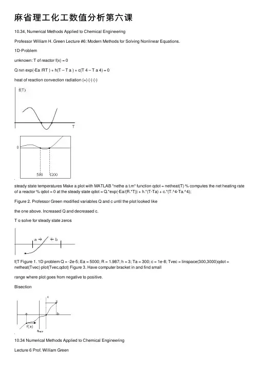
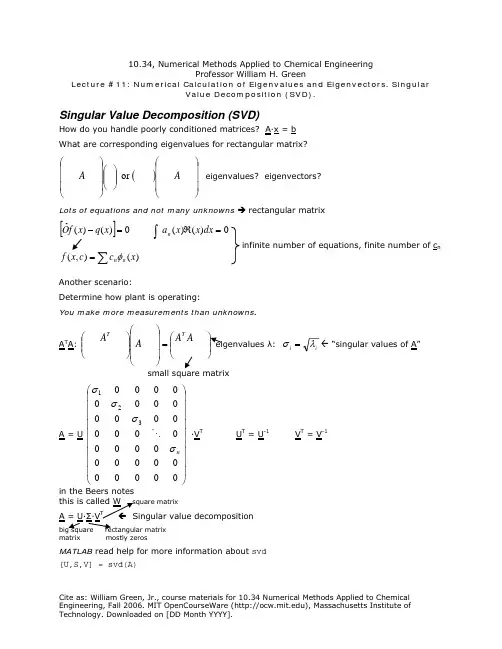
⿇省理⼯化⼯数值分析第六课10.34, Numerical Methods Applied to Chemical EngineeringProfessor William H. Green Lecture #6: Modern Methods for Solving Nonlinear Equations.1D-Problemunknown: T of reactor f(x) = 0Q rxn exp(-Ea /RT ) + h(T – T a ) + c(T 4 – T a 4) = 0heat of reaction convection radiation (+) (-) (-)steady state temperatures Make a plot with MATLAB *nethe a t.m* function qdot = netheat(T) % computes the net heating rate of a reactor % qdot = 0 at the steady state qdot = Q.*exp(-Ea/(R.*T)) + h.*(T-Ta) + c.*(T.^4-Ta.^4);Figure 2. Professor Green modified variables Q and c until the plot looked likethe one above. Increased Q and decreased c.T o solve for steady state zerosf(T Figure 1. 1D problem Q = -2e-5; Ea = 5000; R = 1.987; h = 3; Ta = 300; c = 1e-8; Tvec = linspace(300,3000)qdot = netheat(Tvec) plot(Tvec,qdot) Figure 3. Have computer bracket in and find smallrange where plot goes from negative to positive.Bisection10.34 Numerical Methods Applied to Chemical EngineeringLecture 6 Prof. William GreenPage 2 of 4start a,b such that f(a)<0 and f(b) < 0 2b a x +=Figure 4. Funif f(x) · f(a) > 0 a = xelse b = xThis is a problem of TOLERANCEif((b-a) < tol) stopTypes of tolerance Absolute tolerance Relative tolerance atol: has unitsif |f(x)| < atol·f rtol: if(b-a) < rtol*|a| has to be BIG numberIn MATLAB while abs(b-a) > atolx x = (a+b)/2 if f(x)·f(a) > 0 a = x else b = x end *bisect.m* function x = bisect(f,a,b,atolx,rtolx, atolf) %solves f(x) = 0 while abs(b-a) > atolx x = 0.5*(b+a); if((feval(f,x)*feval(f,a))>0) a =x; else b=x; end endCommand Window x = bisect(@netheat,300,2000,0.1,0,0) x = 1.2373e+003CHECK: netheat(1237) = -1.0474 í closeKeep in mind: never get actual solution, but can come closeWe can change tolerances to improve results. ? while(abs(b-a)>atolx)&&(abs(b-a)>(rtolx*abs(a)))x = 0.5*(b+a); AND: must satisfy both conditions if(a bs(fev a l(f,x))x = 1.2363e+003 looser tolerance gives less accurate answerBisection cuts interval by 2 each timeEvery time we cut 3 times, we lose a sig figIn bisection, time grows linearly with the number of significant figures.a < x true < bx true = x soln ± b-a/2Newton’s Method (1-D)evaluates slope of f(x)next guess is the x new that satisfies f(x new)=0for a line from f(x guess) with the slope at f(x guess)Figure 5. Newton’s Method.For a good guess Newton’s method doublesthe number of significant figures after everyiteration; however, we lose robustness ifguess is poorf(x) = f(x0)+f’(x0)*(x-x0)+O(Δx2)0 = f(x guess)+f’(x guess)*(x-x guess)If f’(x guess) ≈ 0 -- doesn’t workx new = x guess – f(x guess)/f’(x guess)Figure 6.NO intersectionAnother drawback is one needs a derivative of the function. Secant Methodsame as Newton’s, but uses f’(x) approximate]1[][]1[][)()()('=kkkkapproxxxxfxfxfBisection method works only for 1D problems, but Newton/Secant can be used for problems with greater dimension 10.34 Numerical Methods Applied to Chemical Engineering Lecture 6 Prof. William Green Page 3 of 4 Broyden’s Method (Multi-dimensional) F(x) = F(x 010.34 Numerical Methods Applied to Chemical EngineeringLecture 6 Prof. William GreenPage 4 of 4f(x) = 0 approx J = B 2][1||||x B BΔ+=+k ][k Outer Product:ΔΔΔΔΔΔ (32221)2312111x F x F x F x F x F x FNewton’s Method (Multi-dimensional)O = F(x 0)+J(x 0)·(x-x 0)J*Δx = -F(x 0) B [k]Δx = -FLU LU [k+1] without redoing factorization Done in detail in homework problem.。

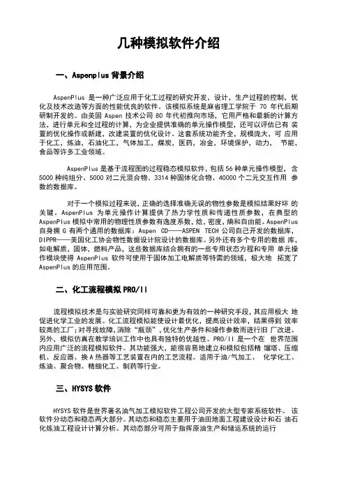
几种模拟软件介绍一、Aspenplus背景介绍AspenPlus是一种广泛应用于化工过程的研究开发，设计，生产过程的控制，优化及技术改造等方面的性能优良的软件。

该模拟系统是麻省理工学院于70年代后期研制开发的。

由美国Aspen技术公司80年代初推向市场，它用严格和最新的计算方法，进行单元和全过程的计算，为企业提供准确的单元操作模型，还可以评估已有装置的优化操作或新建，改建装置的优化设计。

这套系统功能齐全，规模庞大，可应用于化工，炼油，石油化工，气体加工，煤炭，医药，冶金，环境保护，动力，节能，食品等许多工业领域。

AspenPlus是基于流程图的过程稳态模拟软件，包括56种单元操作模型，含5000种纯组分、5000对二元混合物、3314种固体化合物、40000个二元交互作用参数的数据库。

对于一个模拟过程来说，正确的选择准确无误的物性参数是模拟结果好坏的关键。

AspenPlus为单元操作计算提供了热力学性质和传递性质参数，在典型的AspenPlus模拟中常用的物理性质参数有逸度系数，焓，密度，熵和自由能。

AspenPlus 自身拥G有两个通用的数据库：Aspen CD——ASPEN TECH公司自己开发的数据库，DIPPR——美国化工协会物性数据设计院设计的数据库。

另外还有多个专用的数据库，如电解质，固体，燃料产品，这些数据库结合拥有的一些专用状态方程和专用单元操作模块使得AspenPlus软件可使用于固体加工电解质等特需的领域，极大地拓宽了AspenPlus的应用范围。

二、化工流程模拟PRO/II流程模拟技术是与实验研究同样可靠和更为有效的一种研究手段，其应用极大地促进化学工业的发展。

化工流程模拟能使设计最优化，提高设计效率，结果得到效率较高的工厂；对寻找故障，消除“瓶颈”，优化生产条件和操作参数而进行旧厂改进。

另外，模拟仿真在教学培训工作中也具有独特的优越性。

PRO/II是一个在世界范围内应用广泛的流程模拟软件。

土工数值分析（一）土体稳定的极限平衡和极限分析目录1 前言 (2)2 理论基础－塑性力学的上、下限定理 (4)2.1 一般提法 (4)2.2 塑性力学的上、下限定理 (5)2.3 边坡稳定分析的条分法 (7)3 土体稳定问题的下限解－垂直条分法 (9)3.1 垂直条分法的静力平衡方程及其解 (9)3.2 数值分析方法 (11)3.3 垂直条分法的有关理论问题 (15)3.4 垂直条分法在主动土压力领域中的应用 (19)4 土体稳定分析的上限解－斜条分法 (23)4.1 求解上限解的基本方程式 (23)4.2 上限解和滑移线法的关系 (24)4.3 边坡稳定分析的上限解 (27)4.4 地基承载力的上限解 (27)5 确定临界滑动模式的最优化方法 (30)5.1 确定土体的临界失稳模式的数值分析方法 (30)5.2 确定最小安全系数的最优化方法 (31)6 程序设计和应用 (39)6.1 概述 (39)6.2 计算垂直条分法安全系数的程序S.FOR (39)6.3 计算斜条分法安全系数的程序E.FOR (53)1土工数值分析（一）：土体稳定的极限平衡和极限分析法1前言边坡稳定、土压力和地基承载力是土力学的三个经典问题。

很多学者认为这三个领域的分析方法属于同一理论体系，即极限平衡分析和极限分析方法，因此，应该建立一个统一的数值分析方法。

Janbu 曾在1957年提出过土坡通用分析方法。

Sokolovski(1954)应用偏微分方程的滑移线理论提出了地基承载力、土压力和边坡稳定的统一的求解方法。

W. F. Chen (1975) 在其专著中全面阐述了在塑性力学上限和下限定理基础上建立的土体稳定分析一般方法。

但是，上述这些方法只能对少数具有简单几何形状、介质均匀的问题提供解答，故没有在实践中获得广泛的应用。

下面分析这三个领域分析方法的现状以及建立一个统一的体系的可能性。

有关边坡稳定分析的理论的研究工作，从早期的瑞典法，到适用的园弧滑裂面的Bishop简化法，到适用于任意形状、全面满足静力平衡条件的Morgenstern - Price法(1965)，其理论体系逐渐趋于严格。