Mutual Fund Performance
- 格式:pdf
- 大小:287.27 KB
- 文档页数:37
有用的金融术语翻译financial markets 金融市场savings and loans 储蓄存款与借款credit unions 信用社mortgages 抵押贷款(指房屋,土地等)auto loans 汽车消费贷款certificates of deposit 存款单银行对存款人将资金存放于银行一定期间所发给的证明文件,可分为可转让定存单(Negotiable CD)与不可转让定存单(Non-negotiable)managerial finance 财务管理wave of mergers 合并风浪,公司或组织的合并Common equity 普通股Par value股票的面值Retained earnings保留盈餘資產負債表中股東權益重要項目之一,表示公司的獲利保留,未以股利方式配發,並將保留盈餘做為公司長期營運資金或固定投資的資金來源。
(又稱未分配盈餘、盈餘公積、累計盈餘或保留淨利)Additional paid-in capital 附加的缴入资本(属于所有者权益)Discounted securities折价证券Treasury bills 国库券Repurchase agreement重购回协定。
Repurchase Agreement。
指资产的卖方同意在某特定日期,以特定价格再买回其所卖出资产的协议。
...Federal funds 联邦资金Banker’s acceptance银行承兑Commercial paper商业票据Certificate of deposit存款单Negotiable CD 可转让存单Eurodollar deposit 欧元存款Money market mutual funds货币市场的开放式资金Term loan定期贷款Coupon rate 票面利率General obligation bond市政债券可分两大类: (1)一般信用担保债券(generalobligation bond): 并无与特别项目挂钩的市政债券,其本息的偿付来自发行当局的综合收入--主要为地方政府的各种税收;Debenture 公司债券Subordinated debenture subordinated debenture次位债券. 一种无担保债券,发行机构万一破产,求偿顺位低于其他债券。
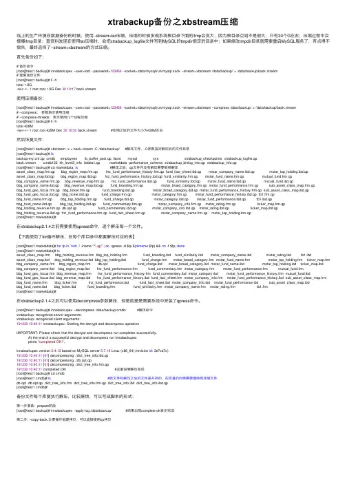
xtrabackup备份之xbstream压缩线上的⽣产环境在数据备份的时候,使⽤--stream=tar压缩,压缩的时候发现系统根⽬录下⾯的/tmp会变⼤;因为根⽬录空间不是很⼤,只有30个G左右;压缩过程中会撑爆/tmp⽬录;查资料发现在使⽤tar压缩时,会把xtrabackup_logfile⽂件写到MySQL的tmpdir指定的⽬录中;如果修改tmpdir⽬录就需要重启MySQL服务了,有点得不偿失,最终选择了--stream=xbstream的⽅式压缩。
⾸先备份如下:# 备份命令[root@test1 backup]# innobackupex --user=root --password=123456 --socket=/data/mysql/run/mysql.sock --stream=xbstream /data/backup/ > /data/backup/back.xtream# 查看备份⽂件[root@test1 backup]# ll -htotal 1.8G-rw-r--r-- 1 root root 1.8G Dec 3010:17 back.xtream使⽤压缩备份:[root@test1 backup]# innobackupex --user=root --password=123456 --socket=/data/mysql/run/mysql.sock --stream=xbstream --compress /data/backup/ > /data/backup/back.xtream# --compress:参数表⽰使⽤压缩# --compress-threads:表⽰使⽤⼏个线程压缩[root@test1 backup]# ll -htotal 428M-rw-r--r-- 1 root root 428M Dec 3010:20 back.xtream #压缩之后的⽂件⼤⼩为430M左右然后恢复⽂件:[root@test1 backup]# xbstream -x < back.xtream -C /data/backup/ #解压⽂件,-C参数指定解压后的⽂件⽬录[root@test1 backup]# lsf.qp cmdb employees ib_buffer_pool.qp lianxi mysql sys xtrabackup_checkpoints xtrabackup_logfile.qpback.xtream cmdb123 hk_level2_info ibdata1.qp marketdata performance_schema xtrabackup_binlog_info.qp xtrabackup_info.qp[root@test1 backup]# cd marketdata; ls #解压之后,qp⽂件并没有解压需要继续解压asset_class_map.frm.qp bbg_region_map.frm.qp fnz_fund_performance_history.frm.qp fund_fact_sheet.ibd.qp mstar_company_name.ibd.qp mstar_top_holding.ibd.qpasset_class_map.ibd.qp bbg_region_map.ibd.qp fnz_fund_performance_history.ibd.qp fund_similarity.frm.qp mstar_fund_name.frm.qp mutual_fund.frm.qpbbg_company_name.frm.qp bbg_revenue_map.frm.qp fnz_fund_performance.ibd.qp fund_similarity.ibd.qp mstar_fund_name.ibd.qp mutual_fund.ibd.qpbbg_company_name.ibd.qp bbg_revenue_map.ibd.qp fund_branding.frm.qp mstar_broad_category.frm.qp mstar_fund_performance.frm.qp sub_asset_class_map.frm.qpbbg_fund_geo_focus.frm.qp bbg_ticker.frm.qp fund_branding.ibd.qp mstar_broad_category.ibd.qp mstar_fund_performance_history.frm.qp sub_asset_class_map.ibd.qpbbg_fund_geo_focus.ibd.qp bbg_ticker.ibd.qp fund_charge.frm.qp mstar_category.frm.qp mstar_fund_performance_history.ibd.qp tb1.frm.qpbbg_fund_name.frm.qp bbg_top_holding.frm.qp fund_charge.ibd.qp mstar_category.ibd.qp mstar_fund_performance.ibd.qp tb1.ibd.qpbbg_fund_name.ibd.qp bbg_top_holding.ibd.qp fund_commentary.frm.qp mstar_company_info.frm.qp mstar_rating.frm.qp ticker_map.frm.qpbbg_holding_revenue.frm.qp db.opt.qp fund_commentary.ibd.qp mstar_company_info.ibd.qp mstar_rating.ibd.qp ticker_map.ibd.qpbbg_holding_revenue.ibd.qp fnz_fund_performance.frm.qp fund_fact_sheet.frm.qp mstar_company_name.frm.qp mstar_top_holding.frm.qp[root@test1 marketdata]#在xtrabackup2.1.4之前需要使⽤qpress命令,逐个解压每⼀个⽂件。
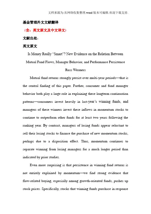
基金管理外文文献翻译(含:英文原文及中文译文)文献出处:英文原文Is Money Really “Smart”? New Evidence on the Relation Between Mutual Fund Flows, Manager Behavior, and Performance PersistenceRuss WermersMutual fund returns strongly persist over multi-year periods—that is the central finding of this paper. Further, consumer and fund manager behavior both play a large role in explaining these longterm continuation patterns—consumers invest heavily in last-year’s winning funds, and managers of these winners invest these inflows in momentum stocks to continue to outperform other funds for at least two years following the ranking year. By contrast, managers of losing funds appear reluctant to sell their losing stocks to finance the purchase of new momentum stocks, perhaps due to a disposition effect. Thus, momentum continues to separate winning from losing managers for a much longer period than indicated by prior studies.Even more surprising is that persistence in winning fund returns is not entirely explained by momentum—we find strong evidence that flow-related buying, especially among growth-oriented funds, pushes up stock prices. Specifically, stocks that winning funds purchase in responseto persistent flows have returns that beat their size, book-to-market, and momentum benchmarks by two to three percent per year over a four-year period. Cross-sectional regressions indicate that these abnormal returns are strongly related to fund inflows, but not to the past performance of the funds—thus, casting some doubt on prior findings of persistent manager talent in picking stocks. Finally, at the style-adjusted net returns level, we find no persistence, consistent with the results of prior studies. On balance, we confirm that money is smart in chasing winning managers, but that a “copycat” s trategy of mimicking winning fund stock trades to take advantage of flow-related returns appears to be the smartest strategy.Eighty-eight million individuals now hold investments in U.S. mutual funds, with over 90 percent of the value of these investments being held in actively managed funds. Further, actively managed equity funds gain the lion’s share of consumer inflows—flows of net new money to equity funds (inflows minus outflows) totalled $309 billion in 2000, pushing the aggregate value of investments held by these funds to almost $4 trillion at year-end 2000. While the majority of individual investors apparently believe in the virtues of active management in general, many appear to hold even stronger beliefs concerning the talents of subgroups of fund managers—they appear to believe that, among the field of active managers, superior managers exist that can “beat the market” for long periods of time. In particular, Morningstar and Lipper compete vigorouslyfor the attention of these true believers by providing regular fund performance rankings, while popular publications such as Money Magazine routinely profile “star” mutual fund managers. In addition, investor dollars, while not very quick to abandon past losing funds, aggressively chase past winners (see, for example, Sirri and Tufano (1998)).Are these “performance-chasers” wasting their money and time, or is money “smart”? Several past papers have attempted to tackle this issue, with somewhat differing results. For example, Grinblatt and Titman (1989a, 1993) find that some mutual fund managers are able to consistently earn positive abnormal returns before fees and expenses, while Brown and Goetzmann (1995; BG) attribute persistence to inferior funds consistently earning negative abnormal returns. Gruber (1996) and Zheng (1999) examine persistence from the viewpoint of consumer money flows to funds, and find that money is “smart”—that is, money flows disproportionately to funds exhibiting superior future returns. However, the exact source of the smart money effect remains a puzzle—does smart money capture manager talent or, perhaps, simply momentum in stock returns?1 More recently, Carhart (1997) examines the persistence in net returns of U.S. mutual funds, controlling for the continuation attributable to priced equity styles (see, for example, Fama and French (1992, 1993, 1996), Jegadeesh and Titman (1993), Daniel andTitman (1997), and Moskowitz and Grinblatt (1999)). Carhart finds little evidence of superior funds that consistently outperform their style benchmarks—specifically, Carhart finds that funds in the highest net return decile (of the CRSP mutual fund database) during one year beat funds in the lowest decile by about 3.5 percent during the following year, almost all due to the one-year momentum effect documented by Jegadeesh and Titman (1993) and to the unexplained poor performance of funds in the lowest prior-year return decile.2 Thus, Carhart (1997) suggests that money is not very smart. Recent studies find somewhat more promising results than Carhart (1997). Chen, Jegadeesh, and Wermers (1999) find that stocks most actively purchased by funds beat those most actively sold by over two percent per year, while Bollen and Busse (2002) find evidence of persistence in quarterly fund performance. Wermers (2000) finds that, although the average style-adjusted net return of the average mutual fund is negative (consistent with Carhart’s study), high-turnover funds exhibit a net return that is significantly higher than low-turnover funds. In addition, these highturnover funds pick stocks well enough to cover their costs, even adjusting for style-based returns. This finding suggests that fund managers who trade more frequently have persistent stockpicking talents. All of these papers provide a more favorable view of the average actively managed fund than prior research, although none focus on the persistence issue with portfolio holdings data.This study examines the mutual fund persistence issue using both portfolio holdings and net returns data, allowing a more complete analysis of the issue than past studies. With these data, we develop measures that allow us to examine the roles of consumer inflows and fund manager behavior in the persistence of fund performance. Specifically, we decompose the returns and costs of each mutual fund into that attributable to (1) manager skills in picking stocks having returns that beat their style-based benchmarks (selectivity), (2) returns that are attributable to the characteristics (or style) of stockholdings, (3) trading costs, (4) expenses, and (5) costs that are associated with the daily liquidity offered by funds to the investing public (as documented by Edelen (1999)). Further, we construct holdings-based measures of momentum-investing behavior by the fund managers. Together, these measures allow an examination of the relation between flows, manager behavior, and performance persistence.In related work, Sirri and Tufano (1998) find that consumer flows react about as strongly to one-year lagged net returns as to any other fund characteristic. In addition, the model of Lynch and Musto (2002) predicts that performance repeats among winners (but not losers), while the model of Berk and Green (2002) predicts no persistence (or weak persistence) as consumer flows compete away any managerial talent. Consistent with Sirri and Tufano (1998), and to test the competing viewpoints of Lynchand Musto (2002) and Berk and Green (2002), we sort funds on their one-year lagged net returns for most tests in this paper. While other ways of sorting funds are attempted.DataWe merge two major mutual fund databases for our analysis of mutual fund performance. Details on the process of merging these databases is available in Wermers (2000). The first database contains quarterly portfolio holdings for all U.S. equity mutual funds existing at any time between January 1, 1975 and December 31, 1994; these data were purchased from Thomson/CDA of Rockville, Maryland. The CDA dataset lists the equity portion of each fund’s holdings (i.e., the shareholdings of each stock held by that fund) along with a listing of the total net assets under management and the self-declared investment objective at the beginning of each calendar quarter. CDA began collecting investment-objective information on June 30, 1980; we supplement these data with hand-collected investment objective data from January 1, 1975.The second mutual fund database is available from the Center for Research in Security Prices (CRSP) and is used by Carhart (1997). The CRSP database contains monthly data on net returns, as well as annual data on portfolio turnover and expense ratios for all mutual funds existing at any time between January 1, 1962 and December 31, 2000. Further details on the CRSP mutual fund database are available from CRSP.These two databases were merged to provide a complete record of the stockholdings of a given fund, along with the fund’s turnover, expense ratio, net returns, investment objective, and total net assets under management during the entire time that the fund existed during our the period of 1975 to 1994 (inclusive).5 Finally, stock prices and returns were obtained from the CRSP stock files.Performance-Decomposition Methodology In this study, we use several measures that quantify the ability of a mutual fund manager to choose stocks, as well as to generate superior performance at the net return level. These measures, in general, decompose the return of the stocks held by a mutual fund into several components in order to both benchmark the stock portfolio and to provide a performance attribution for the fund. The measures used to decompose fund returns include:1. the portfolio-weighted return on stocks currently held by the fund, in excess of returns (during the same time period) on matched control portfolios having the same style characteristics (selectivity)2. the portfolio-weighted return on control portfolios having the same characteristics as stocks currently held by the fund, in excess of time-series average returns on those control portfolios (style timing)3. the time-series average returns on control portfolios having the same characteristics as stocks currently held (style-based returns)4. the execution costs incurred by the fund5. the expense ratio charged by the fund6. the net returns to investors in the fund, in excess of the returns to an appropriate benchmark portfolio.The first three components of performance, which decompose the return on the stocks held by a given mutual fund before any trading costs or expenses are considered, are briefly described next. We estimate the execution costs of each mutual fund during each quarter by applying recent research on institutional trading costs to our stockholdings data—we also describe this procedure below. Data on expense ratios and net returns are obtained directly from the merged mutual fund database. Finally, we describe the Carhart (1997) regression-based performance measure, which we use to benchmark-adjust net returns.The Ferson-Schadt Measure Ferson and Schadt (FS, 1996) develop a conditional performance measure at the net returns level. In essence, this measure identifies a fund manager as providing value if the manager provides excess net returns that are significantly higher than the fund’s matched factor benchmarks, both unconditional and conditional. The conditional benchmarks control for any predictability of the factor return premia that is due to evolving public information. Managers, therefore, are only labeled as superior if they possess superior private information on stock prices, and not if they change factor loadings over time in response to public information. FS also find that these conditionalbenchmarks help to control for the response of consumer cashflows to mutual funds. For example, when public information indicates that the market return will be unusually high, consumers invest unusually high amounts of cash into mutual funds, which reduces the performance measure, “alpha,” from an unconditional model (such as the Carhart model). This reduction in alpha occurs because the unconditional model does not control for the negative market timing induced by the flows. Edelen (1999) provides further evidence of a negative impact of flows on measured fund performance. Using the FS model mitigates this flow-timing effect. The version of the FS model used in this paper starts with the unconditional Carhart four-factor model and adds a market factor that is conditioned on the five FS economic variables.Decomposing the Persistence in Mutual Fund ReturnsSirri and Tufano (1998) find that consumer flows react about as strongly to one-year lagged net returns as to any other fund characteristic. In addition, the model of Lynch and Musto (2002) predicts that performance repeats among winners (but not losers), while the model of Berk and Green (2002) predicts no persistence (or weak persistence) as consumer flows compete away any managerial talent. Consistent with Sirri and Tufano (1998), and to test the competing viewpoints of Lynch and Musto (2002) and Berk and Green (2002), we sort funds on their one-year lagged net returns for the majority of tests in the remainder ofthis paper. When appropriate, we provide results for other sorting approaches as well.中文译文资金真的是“聪明”吗?关于共同基金流动,经理行为和绩效持续性关系的新证据作者:Russ Wermers此外,基金的复苏在多年期间强烈持续- 这是本文的核心发现。
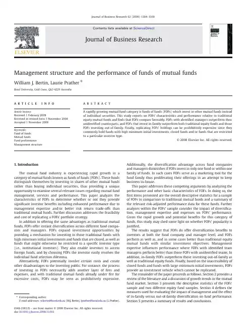
Management structure and the performance of funds of mutual fundsWilliam J.Bertin,Laurie Prather ⁎Bond University,Gold Coast,QLD 4229Australiaa b s t r a c ta r t i c l e i n f o Article history:Received 1February 2008Received in revised form 1November 2008Accepted 1November 2008Keywords:Fund of funds Mutual fundsFund performanceManagement structureA rapidly growing mutual fund category is funds of funds (FOFs)which invest in other mutual funds instead of individual securities.This study reports on FOFs'characteristics and performance relative to traditional equity mutual funds and finds that FOFs compare favorably.FOFs with identi fied managers outperform their unidenti fied counterparts,and FOFs that invest in-family outperform both traditional equity funds and those FOFs investing out-of-family.Finally,replicating FOFs'holdings can be prohibitively expensive since they commonly hold funds with high minimum initial investments,closed funds and/or funds that are restricted to a particular investor type.©2008Elsevier Inc.All rights reserved.1.IntroductionThe mutual fund industry is experiencing rapid growth in a category of mutual funds known as funds of funds (FOFs).These funds distinguish themselves by investing in shares of other mutual funds rather than buying individual securities,thus providing a unique opportunity to examine several relevant issues regarding mutual fund management,services and performance.This paper analyzes the characteristics of FOFs to determine whether or not they provide signi ficant investor bene fits including enhanced performance due to management expertise and/or better risk return trade-offs than traditional mutual funds.Further discussion addresses the feasibility and cost of replicating a FOFs'portfolio strategy.In addition to offering the same advantages as traditional mutual funds,FOFs offer instant diversi fication across different fund compa-nies and managers.FOFs expand investment opportunities by providing a mechanism for investing in those traditional funds with high minimum initial investments and funds that are closed,as well as funds that might otherwise be restricted to a speci fic investor type (i.e.,institutional investors).They also enable investors to access foreign funds,and by choosing FOFs the investor easily resolves the individual fund selection dilemma.Alternatively,FOFs potentially involve certain costs and create other disadvantages to the investing public.For instance,the process of investing in FOFs necessarily adds another layer of fees and expenses,and with traditional mutual funds already under fire for excessive costs,FOFs may be seen as prohibitively expensive.Additionally,the diversi fication advantage across fund companies and managers diminishes if FOFs invest in only one fund or within one family of funds.In such cases FOFs serve as a marketing tool for the fund family thus proliferating their offerings in an attempt to keep business in-house.This paper addresses these competing arguments by analyzing the performance and other basic characteristics of FOFs.In doing so,the first items presented are the overall descriptive statistics for a sample of FOFs in comparison to traditional mutual funds and a summary of the relevant risk-adjusted performance data for these funds.Further analyses within the FOFs'sample consider the impact of diversi fica-tion,management expertise and expenses on FOFs'performance.Given the rapid growth and potential bene fits for this category of funds,this study may shed some light on whether FOFs'popularity is justi fied.The results suggest that FOFs do offer diversi fication bene fits to investors at both the fund company and manager level,and FOFs perform as well as,and in some cases better than traditional equity mutual funds with similar investment objectives.Management expertise in fluences performance where FOFs with identi fied team managers perform better than those FOFs with unidenti fied teams.In addition,in-family FOFs outperform those investing out-of-family as well as traditional equity funds.Finally,based on the inaccessibility of closed funds and funds with large minimum initial investments,FOFs provide an investment vehicle which cannot be replicated.The remainder of the paper proceeds as follows.Section 2provides a review of the literature and a discussion of growth trends in the mutual fund market.Section 3presents the descriptive statistics of the FOFs'sample and two different equity fund samples.Section 4de fines the measures used for evaluating the impact of management and the effect of in-family versus out-of-family diversi fication on fund performance.Section 5presents a summary of results and conclusions.Journal of Business Research 62(2009)1364–1369⁎Corresponding author.E-mail addresses:wbertin@.au (W.J.Bertin),lprather@.au (L.Prather).0148-2963/$–see front matter ©2008Elsevier Inc.All rights reserved.doi:10.1016/j.jbusres.2008.11.003Contents lists available at ScienceDirectJournal of Business Research2.Literature review and market trendsPrior literature on traditional mutual fund performance is quite extensive beginning with the early works of Treynor (1965),Sharpe (1966)and Jensen (1968),which suggest that mutual funds do not beat the market.In providing a summary of the early performance related mutual fund literature,Ippolito (1993),by contrast,reaches the opposite conclusion.More recent studies examine performance by analyzing the impact of costs (fees,turnover and expense ratios)and other mutual fund characteristics with findings that frequently contradict one another (see for example,Carhart,1997;Grinblatt and Titman,1994;Hooks,1996;Malkiel,1993,1995;Payne et al.,1999;Wermers,2000).To explain these contradictory results,Brown et al.(1992),Carhart (1997),Elton et al.(1996,1993),Golec (1996),Grinblatt and Titman (1989,1994),Lehman and Modest (1987)and Malkiel (1995)attribute abnormal performance and persistence to benchmark error and/or the overstatement of returns resulting from survivorship bias.The latest studies including,Bär et al.(2006),Cohen et al.(2005),Friesen and Sapp (2007),Gaspar et al.(2006)and Kacperczyk et al.(2005)continue the performance discussion by considering a variety of fund and management speci fic features such as industry concen-tration,management structure,family cross-subsidization,mimicking top performing funds and market timing.Brown et al.(2004)examine funds of hedge funds citing some of the same potential advantages/disadvantages as noted above for FOFs.They find that the additional fees including high incentive fees leave funds of hedge funds with worse performance records than individual hedge funds.Although their hedge fund study relates,no prior mutual fund studies have systematically analyzed FOFs (funds that invest in traditional mutual funds).In addition to being the first examination of FOFs,this paper contributes to the existing literature by comparing FOFs'performance relative to a sample of traditional equity mutual funds as well as to the overall market.Finally,the study analyzes FOFs'performance in terms of fund management structure and provides a systematic approach for selecting the best FOFs.2.1.FOFs growth trendsThe Morningstar Principia Mutual Funds Advanced (MS)reports performance information for 55multi-class domestic and interna-tional equity FOFs.These funds were offered by 17fund families and accounted for approximately $15billion in mutual fund assets.At the end of 2003,the number of FOFs had grown to 526offerings from 67fund families with FOFs'assets totalling over $85billion representing a 28.6%annual growth rate in FOFs'assets over this seven-year period.In comparison,the number of multi-class equity funds across the same investment objective categories as the FOFs increased from 2138to 6492(with assets increasing from $1.14trillion to $2.50trillion)over the 1996–2003period.This increase represents an 11.87%annual growth rate in assets,or less than half that of the FOFs over the same period.In comparison to similarly classi fied equity funds,FOFs in 1996accounts for approximately 1.3%of total mutual fund assets,but by the end of 2003this proportion had grown to 3.4%.Several factors may be responsible for such an increase including performance and perfor-mance-related demand among investors resulting in an increased flow of funds.Additionally,as mutual fund companies attempt to meet increased demand,they may initiate new or expand upon existing FOFs'offerings (or in some cases proliferate their offerings to compete for fund flows).Finally,unrelated to performance,FOFs'growth and popularity may simply be due to the fact that they offer (or are perceived as offering)something different than the standard mutual fund.3.Descriptive statisticsTo analyze fund composition,performance and cost structure,this study compares the sample FOFs to two groups of equity funds including a broad group of equity funds and a subset of these funds with the same investment objectives as the sample of FOFs.Table 1provides descriptive information for the FOFs and the equity fund samples.Focusing strictly on the FOFs,first in 1996andTable 1Descriptive statistics for FOFs and traditional equity funds.Fund of funds Equity funds Equity fund subset 199620031996200319962003Total assets$14.65(bil)$85.32(bil)$1.70(tril)$3.56(tril)$1.14(tril)$2.50(tril)Number of funds a(55)(526)(4103)(11,011)(2138)(6492)Portfolio characteristics Med.mkt.cap.(mil)$9008$14,823$7762$18,785$10,355$23,957Total holdings (#)bNMF 18139165132170Min.purchase (median)$1000$1000$1000$1000$1000$1000Min.purchase $3063$231,415$169,349$916,783$201,902$921,190Performance PE25.8017.8025.4019.6025.2019.40σ(3-year)(%)8.5112.3812.4119.5611.4918.173-year mean return c 11.49−0.3012.90−2.0114.64−3.50MS rating (3-year) 3.00 3.26 3.03 2.96 3.15 2.97Cost structureFront-end fees (%)0.49 1.01 1.46 1.11 1.44 1.11Deferred load (%)0.380.860.880.970.830.9612b-1fees (%)0.250.330.370.420.350.41Expense ratio (%) 1.160.82 1.54 1.58 1.40 1.45Turnover (%)72498412190170Portfolio characteristics,performance and cost variables in the years 1996and 2003for three groups of mutual funds:funds of funds (FOFs),equity funds and a subset of equity funds with the same investment objectives as the FOFs (figures are averages unless otherwise noted).aThese numbers consider all multi-class funds within each group.The results presented in the remainder of the paper consider only those funds in each group with distinct investment portfolios.Thus,the samples used in the performance comparisons consist of 172FOFs and 2369traditional equity funds.bFor FOFs,the median number of funds held;for equity funds,the average number of securities held.cFor all funds,returns are net of asset-based expenses and fees.For the FOFs,the returns are also net of loads assessed by the traditional funds.1365W.J.Bertin,L.Prather /Journal of Business Research 62(2009)1364–1369then again in 2003,growth is apparent from the number of fund offerings (nearly a ten-fold increase)and the increase in total assets.Further,this growth occurs despite increasing loads.In comparison to the broad equity fund group and the equity subset,FOFs exhibit several distinguishing features.For example,Table 1shows that FOFs are substantially smaller than their equity counterparts,which on a percentage basis could contribute to their larger annual total asset growth (approximately 29%annually compared to the 11%for equity funds and 12%for the equity subset over 1996to 2003).In addition to performance as a driver for this growth differential,increased demand for and flows into FOFs are also contributing factors.Table 1further suggests that FOFs hold more funds that invest in smaller companies than the other two equity groups,as illustrated by the lower average median market capitaliza-tion measure.Finally,the average minimum initial purchase is signi ficantly smaller for FOFs indicating that the two equity groups are comprised of funds requiring larger initial investments,perhaps targeting institutional investors.In measuring FOFs'performance,returns are net of not only their own asset-based expenses and fees,but also all expenses,fees,and loads charged by the individual funds in their portfolio.Table 1indicates that FOFs on average carry a higher Morningstar rating,which is consistent with FOFs average three-year mean return exceeding that of the equity or the equity subset group of funds.These higher returns are accompanied by lower volatility suggesting that FOFs'risk-adjusted performance exceeds that of both traditional equity fund groups.As the final section of Table 1indicates,the cost structure of FOFs has changed dramatically since 1996.For example,by 2003front-end fees and deferred loads had more than doubled while 12b-1fees increased by 32%.Despite these increases in fees and loads,FOFs'expenses are still below those of the two equity groups.In addition,the expense ratio and turnover for FOFs decrease from 1.16%to 0.82%and 72%to 49%,respectively,from 1996to 2003.These figures are well below the expense ratio and turnover figures for the traditional equity fund groups,which have experienced increases in both of these cost categories over the same period.To further explore these cost/performance observations,the paper next provides a detailed statistical analysis for both the FOFs'group and the equity subset.4.Performance evaluation 4.1.Performance analysisThe FOFs and the equity funds comparisons are based on two common risk-adjusted performance measures,which include Jensen's alpha (α)and the Sharpe ratio.These measures are estimated for each fund over the period 1996–2003.While the equity fund subset permits the matching of the fund samples based on investment objective,we also control for allocation-based performance differ-ences by estimating modi fied Jensen's alphas using a multi-factor version of the capital asset pricing model.Similar to Elton et al.(2003),the multi-benchmark model includes three different equity market factors and one bond market factor;large and small capitalization stock indexes,a foreign stock index and a bond index.These benchmarks capture the impact of the funds'differential holdings of large-cap,small-cap,foreign and bond investments.The model appears as follows:r pt −r ft =α+βpL r Lt −r ft ðÞ+βpS r St −r ft ðÞ+βpF r Ft −r ft ðÞ+βpB r Bt −r ft ðÞ+e pt ð1Þwhere,r pt is the return on the fund being evaluated in period t ,r ft is the return on the riskless asset in period t (3-month T-bill),βpjis the sensitivity to benchmark j ,r jt is the return on the benchmark in period t ,L is a large stock index (S&P 500),S is a small stock index (S&P 600),F is a foreign stock index (MSCI World),B is a bond index (Lehman Brother's LT Govt/Corp.Bond),εptis the random error.Jensen's alpha the intercept term from the model,provides a measure of abnormal performance.The four indexes (S&P 500,S&P600,MSCI World and Lehman Brother's LT Government/Corporate Bond)are mutually exclusive in their constituents and cover the most commonly used benchmarks,thus minimizing the potential for benchmark error.The Sharpe ratio measures risk-adjusted performance using a benchmark based on the ex-post capital market line and is calculated as follows:SR p =ar p −ar f=σp ð2Þwhere,ar paverage monthly fund return(FOFs returns are net of asset-based expenses and fees,and all realized expenses,fees,and loads of the individual funds in their portfolio.The equity fund subset returns are net of all asset-based expenses and fees).ar f average monthly risk-free return (3-month T-Bill)σpstandard deviation of the monthly returns for the fund.This ratio is calculated for each fund over the period 1996–2003.For performance comparisons,the equity funds sample is the subset group of all equity funds with the same investment objectives (designated by Morningstar )as the FOFs'sample.Therefore,the investment objectives for both the FOFs and equity subset samples include the categories of aggressive growth,growth,growth and income,asset allocation and balanced.Both of the above performance measures are calculated for each fund with a performance history of at least one year.The final sample consists of 172FOFs and 2369equity funds for a total of 2541funds holding distinct investment portfolios.Table 2reports the average alphas and coef ficient estimates of the multi-benchmark model and the average Sharpe ratios for FOFs and the equity fund subset.The table also includes test statistics forTable 2Performance analysis.FOFsEquity Fund Subset t -statistic α−0.0004+−0.0008+1.15βpL 0.38+0.62+−9.74⁎⁎⁎βpS 0.19+0.28+−0.66βpB 0.09+0.02+8.65⁎⁎⁎βpF0.13+0.04+9.32⁎⁎⁎Sharpe ratio 0.08+0.07+ 2.49⁎⁎⁎N1722369This table includes Jensen's alphas and beta estimates for the multi-benchmark model and the Sharpe ratios for the 172FOFs and the subset of 2369equity funds from 1996–2003.For the multi-benchmark model,the estimates for the betas are denoted as:L for the large stock index,S for the small stock index,B for the bond index and F for the foreign stock index.Also included is the Wilcoxon two-sample test statistic comparing the mean coef ficient estimates of the FOFs sample and the equity fund subset.Modi fied Jensen's α:r pt −r ft =α+βpL (r Lt −r ft )+βpS (r St −r ft )+βpB (r Bt −r ft )+βpF (r Ft −r ft )+εpt .Sharpe ratio:SR p =(ar p −ar f )/σp .Coef ficients different from zero:+++1%signi ficance,++5%signi ficance,and +10%signi ficance.Coef ficients different across fund samples:⁎⁎⁎1%signi ficance level,⁎⁎5%signi ficance level,and ⁎10%signi ficance level.1366W.J.Bertin,L.Prather /Journal of Business Research 62(2009)1364–1369comparing the two samples.The alpha estimates for both samples are negative and significantly different from zero indicating that on average neither group outperforms the overall market.Still the magnitude of the equity funds subset negative alpha is twice that of the FOFs'sample and a comparison of the Sharpe ratios suggests that the FOFs outperforms the equity funds subset,and this difference is statistically significant.Thisfinding is in contrast to Brown et al.'s (2004)study where the funds of hedge funds significantly under-performed the individual hedge funds,which may be explained by the fact that FOFs are not subject to the incentive fees that significantly erode the returns for the funds of hedge funds.An analysis of non-overlapping subperiods representing up-market and down-market periods provides results consistent with the overall results.Additionally,separate regression tests indicate that the multi-benchmark model adequately captures potential allocation-based performance differentials.Finally,after considering the impact of fund specific variables including turnover,expense ratio and fund age on performance,FOFs still compare favorably to the equity fund subset.(The results of the robustness tests not included here are available upon request).4.2.Management structure and performanceAdvocates of FOFs hype their ability to provide access to top quality managers and to achieve risk reduction through fund manager and fund company diversification.The potential advantage of manage-ment diversification is obvious assuming that managers'performance records are not perfectly correlated.Finance theory would suggest that by holding a portfolio of funds with different managers,poor performance by one manager can be offset by another's good performance.Along these lines,Fant and O'Neal(1999)document substantial risk reduction benefits associated with diversification across fund managers.Although a similar diversification argument can be made at the fund company level,holding different companies' funds may also expand the range of investment opportunities. Additionally,FOFs that invest across different fund companies may provide monitoring services.Agency theory further suggests that FOFs' managers,in their capacity as monitors,reduce potential inefficiencies arising from agency problems between fund managers and fund owners.Thus,agency costs(the added layer of fees and expenses borne by investors)compensate FOFs'managers for the oversight function they provide.Given the relative performance of FOFs,the next empirical tests examine the potential sources of gains,such as diversification(fund companies/managers)and/or management expertise(monitoring/ informational advantages).As previously reported in Table1,the lower standard deviation of returns for FOFs implies diversification benefits.Since the sample FOFs'holdings are highly diversified(FOFs hold an average of18traditional funds,which in turn hold an average of170individual securities),and Eling and Schuhmacher(2007) document Sharpe ratio rankings of fund performance to be virtually identical to a wide array of other performance measures,the following analyses focus on Sharpe ratio comparisons within the FOFs'sample.The MS database provides information regarding management structure for160of172sample FOFs thus allowing funds to be categorized as follows:funds managed by an individual,funds managed by an identified team(typically fewer than4individuals), or unidentified,team-managed funds.In the FOFs'sample the management structure for the160funds consists of60funds being individually managed,32managed by identified teams and68having unidentified team-managers.If performance is purely due to diversification benefits,then management structure should have no impact on the results.Alternatively,if management expertise adds value,then performance differentials should be evident.To evaluate the performance for the three different groupings based upon their management structures,Table3uses a matrix format to report the Sharpe ratios and significance tests for comparisons of management structure within the FOFs'sample.The Sharpe ratios and the number of funds within each management category are listed along the diagonals of the table,and the Wilcoxon signed-rank test statistics for comparing managers are listed on the off-diagonals.The average monthly ratio is highest for the funds managed by individuals and lowest for the unidentified team-managed funds.The ratios for the two groups of funds with identified managers(individual and team)are0.0751and0.0484,respectively, and the null hypothesis of equal means cannot be rejected.The Sharpe ratio for the unidentified team-managed funds however,is0.0202, resulting in the rejection of the null hypothesis of equal means when comparing this group to the identified team-managed group.These results suggest that benefits extend beyond simple manager diversification or company diversification as better performance is achieved by those funds that specifically designate and identify their managers.Since identified teams may be directly responsible for the FOFs'performance,their reputations are at stake.This responsibility provides the motivation to use their management expertise in selecting fund managers and fund companies,as well as evaluating the economy,industry andfirms in which the traditional funds invest. Thesefindings indicate enhanced performance for identified team managers who provide more than naïve diversification.In contrast, fund companies that offer funds with unidentified managers may be attempting to capitalize on the demand for FOFs by creating a product that simply combines their existing funds.In doing so,these FOFs merely offer naïve diversification with no specialized management expertise,and their performance is significantly worse.Baer et al. (2006)find a negative relationship between team management and fund performance,however,they do not differentiate between identified and unidentified teams.In contrast,sample stratification based on identification of team managers allows us to capture a differential impact for those FOFs putting their names and reputations on the line versus those that are merely creating a popular product.To address the benefits of diversification across fund companies, management expertise,and/or monitoring that reduces the potential agency conflict,the following discussion and analysis compares theTable3Performance measures for FOFs as a function of management structure.Individual Identified Team Man.Unidentified Team Man.Individual Manager 0.0751z=1.0288z=0.9812(60)p-value=(0.1518)p-value=(0.1632)Identified Team Management 0.0484z=2.3091(32)p-value=(0.0105)Unidentified Team Management 0.0202 (68)For the sample of160FOFs based on management structure(individual,identified team and unidentified team),the average monthly Sharpe ratios are reported along the diagonals with the number of funds in each group in parentheses.The off-diagonals include the Wilcoxon z-statistics and p-values used to compare differences in the Sharpe ratios for individual versus identified team,individual versus unidentified team and identified team versus unidentified team.Table4Fund company diversification and performance evaluation.ANOVA teststatisticsWilcoxon teststatisticsSharpe ratio St.dev.z p-value F p-value N In-family FOFs0.11080.31 4.16b0.0001 1.81370.0349135 Out-of-family FOFs−0.00400.10−0.23550.815334 This table includes average monthly Sharpe ratios,standard deviations and ANOVA test statistics.The Wilcoxon signed rank test statistics are also included to compare the performance of135FOFs that invest in-family to that of the34FOFs that invest out-of-family.1367W.J.Bertin,L.Prather/Journal of Business Research62(2009)1364–1369performance of FOFs that invest in-family to those that invest out-of-family.While FOFs investing out-of-family can offer diversification at both the manager level and fund company level,funds investing in-family can only offer diversification at the fund manager level.The data clearly demonstrates that FOFs offer diversification across mutual fund managers as only three cases exist where a FOFs'manager has invested in traditional funds solely under his/her own management. Diversification across different fund companies,however,is less apparent as135of the FOFs invest in-family and only34invest outside of the fund family.To analyze these two distinct groups of FOFs,Table4presents their average monthly Sharpe ratios for performance comparisons.The average monthly ratio for the in-family group is0.1108,which is significantly different from zero and larger than that of the out-of-family group at−0.0040.According to the Wilcoxon signed-rank test, the performance differential between the two groups is statistically significant indicating the desirability of FOFs that invest in-family.Although thisfinding seems contrary to the notion of diversifica-tion and monitoring benefits,the dominance of in-family performance may result from asymmetric information regarding in-house fund managers.FOFs that invest in-house may be privy to inside information that would not be available to the FOFs'managers investing out-of-family.Thus the diversification and monitoring benefits of investing out-of-family are more than offset by the losses associated with asymmetric information,although in most cases investing out-of-family is a function of limited in-house availability of mutual funds.For example,in the case of the out-of-family sample, families only provide on average19traditional equity fund offerings compared to120offerings for in-family FOFs.A further consideration is that within a family,the traditional equity funds may be holding similar portfolios thus creating heavier weightings in certain industries or individual securities when compared to a FOF investing out of family.This investment overlap may be contributing to the superior performance of the in-family group,thus further supporting the informational advantage of FOFs investing in-family.In-family FOFs also have the support of larger fund complexes, such that investing in-house could provide certain cost advantages not available to outsiders,including full or partial waiver of expenses,fees and loads.Fund companies may offer such waivers as a marketing tool to encourage predictableflows into the traditional funds within the family.Additionally,fund companies that offerfinancial advisory services mayfind efficiencies by putting smaller investors into FOFs to reduce costs associated with reviewing and rebalancing portfolios.Thus,holding funds through a FOFs'investment can actually reduce overall costs,as Table1 shows FOFs'average cost structure is lower than that of traditional equity funds.Thisfinding is consistent with the results of Gaspar et al.(2006),which document cross-fund subsidization within mutual fund families.The next analysis considers whether management structure has an impact on performance between in-family and out-of-family FOFs. The identification of management structure is possible for129of the 135in-family FOFs and31of the34in the out-of-family group.Table5 contains the Sharpe ratios for both groups classified by individual managers,identified team managers and unidentified team managers. For the in-family FOFs,individual,identified-team,and unidentified team managed funds have ratios of0.1067,0.0416and0.0338, respectively.While this performance measure for the individually managed funds is larger than the other groups,the null hypothesis of equal means cannot be rejected.These results suggest that in-family versus out-of-family investment decisions are more important than management structure in determining FOFs'performance.For the31 funds that invest out-of-family,15are individually managed,five have team-identified structures and11are unidentified team managed with Sharpe ratios of−0.0196,0.0854and−0.0503,respectively. Thus,the FOFs that invest out-of-family with unidentified team management structures exhibit the worst performance.Afinal analysis compares the performance of the FOFs to the equity fund subset.Table6reports the Sharpe ratios and Jensen's alphas for both the in-family and out-of-family FOFs and also for the subset of equity funds.The comparisons provide evidence that the in-family FOFs not only keep pace with the traditional funds,but that they also exhibit superior performance(approximately10%signifi-cance level).By contrast the Sharpe ratio for the out-of-family FOFs is significantly below that of the traditional funds.These results sup-port the priorfindings that those FOFs investing in-family are the preferred choice not only among FOFs,but also among mutual funds in general.Based on the superior performance of in-family FOFs,the logical extension is to increase returns by replicating a FOFs'portfolio with a hypothetical“do-it-yourself”strategy in an attempt to avoid the additional layer of fees and expenses.In theory,replication is possible given that Morningstar provides complete listings of mutual funds'Table5Performance comparisons:in-family versus out-of-family FOFs and management structure.Sharpe ratio St.dev.t p-value NPanel A:129in-family FOFsIndividual managers(IND)0.10670.26 2.800.007645Identified team-managed(IDT)0.04160.11 2.040.051827Unidentified team-managed(UNT)0.03380.13 1.920.060257Wilcoxon signed-rank tests H0:SR IND=SR IDT z=0.0582H0:SR IND=SR UNT z=1.0244H0:SR IDT=SR UNT z=1.1302H a:SR IND N SR IDT p-value=0.4768H a:SR IND N SR UNT p-value=0.1528H a:SR IDT N SR UNT p-value=0.1292Panel B:31out-of-family FOFsIndividual managers(IND)−0.01960.10−0.79710.438715Identified team-managed(IDT)0.08540.03 5.75310.00455Unidentified team-managed(UNT)−0.05030.10−1.68940.122011This table reports Sharpe ratios,standard deviations and test statistics for comparing the impact of management structure(individual,identified team,unidentified team)on FOFs that invest in-family and FOFs that invest out-of-family.Table6Performance comparisons for FOFs and the equity fund subset.Equity fundFOFs Subset Wilcoxon z p-valueIn-familySharpe ratio0.11080.04100.96670.1668Jensen's alpha−0.0003−0.0008 1.24370.1068Out-of-familySharpe ratio0.00400.0410 2.17890.0147Jensen's alpha−0.0008−0.00080.04020.4840This table compares the performance of the in-family and out-of-family FOFs'performance to that of the equity fund subset using both Sharpe ratio and Jensen'salpha as performance measures and also reports test statistics.1368W.J.Bertin,L.Prather/Journal of Business Research62(2009)1364–1369。

Chapter04MutualFundsandOtherInvestmentCompanies Chapter 04Mutual Funds and Other Investment Companies Multiple Choice Questions1. Which one of the following invests in a portfolio that is fixed for the life of the fund?A. Mutual fundB. Money market fundC. Managed investment companyD. Unit investment trust2. ______ are partnerships of investors with portfolios that are larger than most individual investors but are still too small to warrant managing on a separate basis.A. Commingled fundsB. Closed-end fundsC. REITsD. Mutual funds3. A __________ is a private investment pool open only to wealthy or institutional investors that is exempt from SEC regulation and can therefore pursue more speculative policies than mutual funds.A. commingled poolB. unit trustC. hedge fundD. money market fund4. Advantages of investment companies to investors include all but which one of the following?A. Record keeping and administrationB. Low cost diversificationC. Professional managementD. Guaranteed rates of return5. Which of the following typically employ significant amounts of leverage?I. Hedge fundsII. REITsIII. Money market fundsIV. Equity mutual fundsA. I and II onlyB. II and III onlyC. III and IV onlyD. I, II and III only6. The NAV of which funds is fixed at $1 per share?A. Equity fundsB. Money market fundsC. Fixed income fundsD. Commingled funds7. The two principal types of REITs are equity trusts which _______________ and mortgage trusts which _______________.A. invest directly in real estate; invest in mortgage and construction loansB. invest in mortgage and construction loans; invest directly in real estateC. use extensive leverage; distribute less than 95% of income to shareholdersD. distribute less than 95% of income to shareholders; use extensive leverage8. A contingent deferred sales charge is commonly called a ____.A. front-end loadB. back-end loadC. 12b-1 chargeD. top end sales commission9. In the U.S. there are approximately _______ mutual funds offered by less than _______ fund families.A. 12,000; 600B. 7,000; 100C. 8,000; 500D. 9,000; 30010. In 1999, the SEC established rules that should make a mutual fund prospectus _______.A. easier to read and understandB. much more detailedC. disappear over the next 10 yearsD. irrelevant to investors11. Mutual funds provide the following for their shareholders:A. DiversificationB. Professional managementC. Record keeping and administrationD. Mutual funds provide diversification, professional management, and record keeping and administration12. The average maturity of fund investments in a money market mutual fund is _______.A. slightly more than one monthB. slightly more than one yearC. about 9 monthsD. between 2 and 3 years13. Rank the following fund category from most risky to least risky.I. Equity growth fundII. Balanced fundIII. Sector fundIV. Money market fundA. IV, I, III, IIB. III, II, IV, IC. I, II, III, IVD. III, I, II, IV14. Which of the following result in a taxable event for investors?I. Short-term capital gains distributions from the fundII. Dividend distributions from the fundIII. Long-term capital gains distributions from the fundA. I onlyB. II onlyC. I and II onlyD. I, II and III15. The type of mutual fund that primarily engages in market timing is called a/an _______.A. sector fundB. index fundC. ETFD. asset allocation fund16. As of 2008, approximately _____ of mutual fund assets were invested in equity funds.A. 5%B. 54%C. 30%D. 12%17. As of 2008, approximately _____ of mutual fund assets were invested in bond funds.A. 14%B. 19%C. 37%D. 47%18. As of 2008, approximately _____ of mutual fund assets were invested in money market funds.A. 5%B. 26%C. 44%D. 66%19. Management fees for open-end and closed-end funds, typically range between _____ and _____.A. 0.2%; 1.5%B. 0.5%; 5%C. 2%; 5%D. 3%; 8%20. The primary measurement unit used for assessing the value of one's stake in an investment company is___________________.A. Net Asset ValueB. Average Asset ValueC. Gross Asset ValueD. Total Asset Value21. Net Asset Value is defined as ________________________.A. book value of assets divided by shares outstandingB. book value of assets minus liabilities divided by shares outstandingC. market value of assets divided by shares outstandingD. market value of assets minus liabilities divided by shares outstanding22. Assume that you have just purchased some shares in an investment company reporting $500 million in assets, $50 million in liabilities, and 50 million shares outstanding. What is the Net Asset Value (NAV) of these shares?A. $12.00B. $9.00C. $10.00D. $1.0023. Assume that you have recently purchased 100 shares in an investment company. Upon examining the balance sheet, you note the firm is reporting $225 million in assets, $30 million in liabilities, and 10 million shares outstanding. What is the Net Asset Value (NAV) of these shares?A. $25.50B. $22.50C. $19.50D. $1.9524. The Vanguard 500 Index Fund tracks the performance of the S&P 500. To do so the fund buys shares in each S&P 500 company __________.A. in proportion to the market value weight of the firm's equity in the S&P500B. in proportion to the price weight of the stock in the S&P500C. by purchasing an equal number of shares of each stock in the S&P 500D. by purchasing an equal dollar amount of shares of each stock in the S&P50025. Which of the following is not a type of managed investment company?A. Unit investment trustsB. Closed-end fundsC. Open-end fundsD. Hedge funds26. Which of the following funds invest in stocks of fast growing companies?A. Balanced fundsB. Growth equity fundsC. REITsD. Equity income funds27. A fund that invests in securities worldwide, including the United States is called a/an ______.A. international fundB. emerging market fundC. global fundD. regional fund28. The greatest percentage of mutual fund assets are invested in ________.A. bond fundsB. equity fundsC. hybrid fundsD. money market funds29. Sponsors of unit investment trusts earn a profit by ___________________.A. deducting management fees from fund assetsB. deducting a percentage of any gains in asset valueC. selling shares in the trust at a premium to the cost of acquiring the underlying assetsD. charging portfolio turnover fees30. Investors who wish to liquidate their holdings in a unit investment trust may___________________.A. sell their shares back to the trustee at a discountB. sell their shares back to the trustee at net asset valueC. sell their shares on the open marketD. sell their shares at a premium to net asset value31. Investors who wish to liquidate their holdings in a closed-end fund may___________________.A. sell their shares back to the fund at a discount if they wishB. sell their shares back to the fund at net asset valueC. sell their shares on the open marketD. sell their shares at a premium to net asset value if they wish32. __________ fund is defined as one where the fund charges a sales commission to either buy into or exit the fund.A. A loadB. A no-loadC. An indexD. A specialized sector fund33. __________ is a false statement regarding open-end mutual funds.A. They offer investors a guaranteed rate of returnB. They offer investors a well diversified portfolioC. They redeem shares at their net asset valueD. They offer low cost diversification34. __________ funds stand ready to redeem or issue shares at their net asset value.A. Closed-endB. IndexC. Open-endD. Hedge35. Revenue sharing with respect to mutual funds refers to _________.A. fund companies paying brokers if the broker recommends the fund to investorsB. allowing certain classes of investors to engage in market timingC. charging loads to new investors in a mutual fundD. directly marketing funds over the Internet36. Higher portfolio turnoverI. results in greater tax liability for investorsII. results in greater trading costs for the fund, which investors have to pay forIII. is a characteristic of asset allocation fundsA. I onlyB. II onlyC. I and II onlyD. I, II and III37. Low load mutual funds have front-end loads of no more than _____.A. 2%B. 3%C. 4%D. 5%38. Most real estate investment trusts (REITs) have a debt ratio of around _________.A. 10 %B. 30 %C. 50 %D. 70 %39. Measured by assets, about _____ of funds are money market funds.A. 15%B. 25%C. 40%D. 60%40. Which of the following is not a type of real estate investment trust?I. Equity trustII. Debt trustIII. Mortgage trustIV. Unit trustA. I and II onlyB. II onlyC. II and IV onlyD. I, II and III41. ______________________ are often called mutual funds.A. Unit investment trustsB. Open-end investment companiesC. Closed-end investment companiesD. REITs42. Mutual funds account for roughly ______ percent of investment company assets.A. 30B. 50C. 70D. 9043. An official description of a particular mutual fund's planned investment policy can be found in the fund's _____________.A. prospectusB. indentureC. investment statementD. 12b-1 forms44. Mutual funds that hold both equities and fixed-income securities in relatively stable proportions are called____________________.A. income fundsB. balanced fundsC. asset allocation fundsD. index funds45. Mutual funds that vary the proportions of funds invested in particular market sectors according to the fund manager's forecast of the performance of that market sector, are called ____________________.A. asset allocation fundsB. balanced fundsC. index fundsD. income funds46. Specialized sector funds concentrate their investments in _________________.A. bonds of a particular maturityB. geographical segments of the real estate marketC. government securitiesD. securities issued by firms in a particular industry47. If a mutual fund has multiple class shares, which class typically has a front end load?A. Class AB. Class BC. Class CD. Class D48. The commission, or front-end load, paid when you purchase shares in mutual funds, may not exceed __________.A. 3%B. 6%C. 8.5%D. 10%49. You are considering investing in one of several mutual funds. All the funds under consideration have various combinations of front-end and back-end loads and/or 12b-1 fees. The longer you plan on remaining in the fund you choose, the more likely you will prefer a fund with a __________ rather than a __________, everything else equal.A. 12b-1 fee; front-end loadB. front-end load; 12b-1 feeC. back-end load, front-end loadD. 12b-1 fee; back-end load50. Under SEC rules, the managers of certain funds are allowed to deduct charges for advertising, brokerage commissions, and other sales expenses, directly from the fund assets rather than billing investors. These fees are known as____________.A. direct operating expensesB. back-end loadsC. 12b-1 chargesD. front-end loads51. In 2000, the SEC instituted new rules that require funds to disclose _____.A. 12b-1 feesB. the tax impact of portfolio turnoverC. front-end loadsD. back-end loads52. SEC rule 12b-1 allows managers of certain funds to deduct __________ expenses from fund assets, however, these expenses may not exceed __________ of the fund's average net assets per year.A. marketing; 1%B. marketing; 5%C. administrative; 0.5%D. administrative; 2%53. Consider a mutual fund with $300 million in assets at the start of the year, and 12 million shares outstanding. If the gross return on assets is 18% and the total expense ratio is 2% of the year end value, what is the rate of return on the fund?A. 15.64%B. 16.00%C. 17.25%D. 17.50%54. Consider a no-load mutual fund with $200 million in assets and 10 million shares at the start of the year, and $250 million in assets and 11 million shares at the end of the year. During the year investors have received income distributions of $2 per share, and capital gains distributions of $0.25 per share. Assuming that the fund carries no debt, and that the total expense ratio is 1%, what is the rate of return on the fund?A. 36.25%B. 24.90%C. 23.85%D. There is not sufficient information to answer this question55. Consider a no-load mutual fund with $400 million in assets, 50 million in debt, and 15 million shares at the start of the year; and $500 million in assets, 40 million in debt, and 18 million shares at the end of the year. During the year investors have received income distributions of $0.50 per share, and capital gains distributions of $0.30 per share. Assuming that the fund carries no debt, and that the total expense ratio is 0.75%, what is the rate of return on the fund?A. 12.09%B. 12.99%C. 8.25%D. There is not sufficient information to answer this question56. Mutual fund returns may be granted pass-through status, if _________________.A. at least 90 percent of all income is distributed to shareholdersB. at least 30 percent of fund income is derived from sale of securities held for less than 3 monthsC. certain diversification criteria are metD. All of these must be true for pass-through status to be granted57. A/an _____ is an example of an exchange-traded fund.A. SPDR or spiderB. samuraiC. VanguardD. open-end fund58. If you place an order to buy or sell a share of a mutual fund during the trading day the order will be executed atA. the NAV calculated at the market close at 4:00 pm New York time.B. the real time NAV.C. the NAV delayed 15 minutes.D. the NAV calculated at the open of the next day's trading.59. With respect to mutual funds, late trading refers to the practice of ________.A. trading after the close of U.S. markets but before overseas markets have closedB. trading after the close of overseas markets, but before U.S. markets have closedC. accepting buy or sell orders after the market closes and NAV has already been determined for the dayD. paying capital gains distributions to certain investors only after paying privileged investors first60. In the 1970 study, Malkiel found that mutual funds that do well in one period, have an approximately ________ chance of doing well in the subsequent ear period.A. 33%B. 52%C. 65%D. 85%61. In a recent study, Malkiel finds that evidence of persistence in the performance of mutual funds, ________________ in the 1980s.A. grows strongerB. remains about the sameC. becomes slightly weakerD. virtually disappears62. The ratio of trading activity of a portfolio to the assets of the portfolio, is called____________.A. the reinvestment ratioB. the trading rateC. the portfolio turnoverD. the tax yield63. Which of the following ETFs tracks the S&P 500 index?A. QubesB. DiamondsC. VipersD. Spiders64. The Stone Harbor Fund is a closed-end investment company with a portfolio currently worth $300 million. It has liabilities of $5 million and 9 million shares outstanding. If the fund sells for $30 a share, what is its premium or discount as a percent of NAV?A. 9.26% premiumB. 8.47% premiumC. 9.26% discountD. 8.47% discount65. The difference between balanced funds and asset allocation funds is that _____.A. balanced funds invest in bonds while asset allocation funds do notB. asset allocation funds invest in bonds while balanced funds do notC. balanced funds have relatively stable proportions of stocks and bonds while the proportions may vary dramatically for asset allocation fundsD. balanced funds make no capital gains distributions and asset allocation funds make both dividend and capital gains distributions66. The Wildwood Fund sells Class A shares with a front-end load of 5% and Class B Shares with a 12b-1 fees of 1% annually. If you plan to sell the fund after 4 years, are Class A or Class B shares the better choice? Assume a 10% annual return net of expenses.A. Class AB. Class BC. There is no difference.D. There is insufficient information given.67. A mutual fund has total assets outstanding of $69 million. During the year the fund bought and sold assets equal to $17.25 million. This fund's turnover rate was _____.A. 25.00%B. 28.50%C. 18.63%D. 33.40%68. Which type of investment fund is commonly known to invest in options and futures in large scale?A. Commingled fundsB. Hedge fundsC. ETFsD. REITS69. Advantages of ETFs over mutual funds include all but which one of the following?A. ETFs trade continuously so investors can trade throughout the dayB. ETFs can be sold short or purchased on margin, unlike fund sharesD. ETF values can diverge from NAV70. Harold has just taken his company public and owns a large quantity of restricted stock. For purposes of diversification, what fund might he help create in order to diversify his holdings?A. Commingled fundsB. Hedge fundsC. ETFD. REITs71. Which of the following funds is most likely to have a debt ratio of 70% or higher?A. Bond fundB. Commingled fundC. Mortgage backed securitiesD. REIT72. About _________ of mutual fund assets are invested in no-load funds.A. 33%B. 40%C. 50%D. 65%73. From 1971 to 2007 the average return on the Wilshire 5000 index was _________ the return of the average mutual fund.A. identical toB. 1% higher thanC. 1% lower thanD. 3% lower than74. An open-end fund has a NAV of $16.50 per share. The fund charges a 6% load. What is the offering price?A. $14.57B. $15.95C. $17.55D. $16.4975. The offer price of an open-end fund is $18.00 and the fund is sold with a front-end load of 5%? What is the fund's NAV?A. $18.74B. $17.10C. $15.40D. $16.5776. A mutual fund has $50 million in assets at the beginning of the year and 1 million shares outstanding throughout the year. Throughout the year assets grow at 12%. The fund imposes a 12b-1 fee on all shares equal to 1%. The fee is imposed on year end asset values. If there are no distributions what is the end of year NAV for the fund?77. The assets of a mutual fund are $25 million. The liabilities are $4 million. If the fund has 700,000 shares outstanding and pays a $3 dividend, what is the dividend yield?A. 5%B. 10%C. 15%D. 20%78. Which of the following funds are usually most tax efficient?A. Equity fundsB. Bond FundsC. ETFsD. Specialized sector funds79. You invest in a mutual fund that charges a 3% front end load, 1% total annual fees, and a 2% back end load, which decreases 0.5% per year. How much will you pay in fees on a $10,000 investment that does not grow, if you cash out after three years of no gain?A. 103B. 219C. 553D. 63580. You invest in a mutual fund that charges a 3% front end load, 1% total annual fees, and a 0% back end load on Class A shares. The same fund charges 0% front end load, 1% total annual fees, and a 2% back end load on Class B shares. What are the total fees in year one on a Class A investment of $20,000 with no growth in value?A. 658B. 794C. 885D. 90281. You invest in a mutual fund that charges a 3% front end load, 1% total annual fees, and a 0% back end load on Class A shares. The same fund charges 0% front end load, 1% total annual fees, and a 2% back end load on Class B shares. What are the total fees in year one on a Class B investment of $20,000 if you redeem shares with no growth in value?A. 596B. 794C. 885D. 90282. You pay $21,600 to the Laramie Fund which has a NAV of $18.00 per share at the beginning of the year. The fund deducted a front-end load of 4%. The securities in the fund increased in value by 10% during the year. The fund's expense ratio is 1.3% and is deducted from year end asset values. What is your rate of return on the fund if you sell your shares at the end of the year?。

Chapter 20 – Hedge FundsGeneral Characteristics▪Category of investing that represents a broad range of different strategies▪Different asset class▪Lightly regulated pools of capital▪Great flexibility in investment strategies utilized▪Started as limited partnerships in US - now taking form of mutual fund trusts▪Majority of return from manager’s skill not marketWho Can Invest?-sophisticated investor-accredited investorHedge Funds - 2- Retail Investor - Commodity Pools- Closed-end Funds- Principal-protected notesHistory of Hedge FundsAlfred Jones – father of hedge funds - wanted to create a fund that offered protection from the probability of declining markets-combined short selling & leverage- his strategy entailed - in rising market-long securities that will rise more than the market-short securities that will rise less than the market- in falling market-short securities that will decline more than the market-long securities that will fall less than the market- his fund outperformed mutual funds in 50s & 60s- many new funds started in mid-60s –didn’t adhere to Jones model –decimated in bear markets of 1969 & 1974-hedge fund revival in late 80s-hundreds of new funds with highly specialized strategies created-Long-Term Capital Management scandal in 1998-In Canada – 180 funds – about 1% of MF assets-In US – 5,000 funds – about 7.5% of MF assetsPerformance – Table 20.2, p. 20.9 and handoutsHedge Fund Benefits1)low correlation to traditional asset classes2)risk minimization3)absolute returns4)potentially lower volatility & higher returnsHedge Fund Risk1)Market Risk - risk of being invested in particular market2)Manager risk - have a wider investment mandate than MF-manager might start to think invincible or become complacent-might take in more money than can efficiently invest-style drift - manager drift to different investment style than when you bought3)Complexity - investor doesn’t understand techniques being used4)Lack of Transparency - investor can’t fully seea.Manager’s investment styleb.Processes for implementing approachc.Positions in portfoliod.Fees & expensesHedge Funds - 35)Liquidity - of investments- liquidity premium- ability to turn investments into cash quickly at good price- of fund - redemption policy- lockup period- specified maturity date6)Leverage - borrowed too much - received a margin call7)Pricing - difficult to price some securities - illiquid, wide bid/askspread8)Data risk - hedge fund managers are not obligated to report numbers9)Event risk - global, unanticipated events10)Business event risk - unexpected company newsDue diligence - p. 20-12TermsLockup - time period initial funds cannot be redeemedLiquidity dates - once lockup period over, investor can redeem on liquidity datesIncentive fees - management fees based on performanceHigh water mark - can only take performance fees on net new profits- sets bar above which manager gets paid % of profitsHedge Fund CategoriesHedge Funds – 4-If equity mkt , convertible& short- & vice versa -If in equity mkts & i at the same time- i cause P bond-default risk of issuer- If i - flight to quality- will liquidity in other bondsHedge Funds – 6Fund of Funds- 2 types - single-strategy-multi-strategyAdvantages:-due diligence-reduced volatility-professional management-access to hedge funds-diversification-risk controlDisadvantages:-additional costs-no guarantee of positive returns -lack of diversification-additional leveragePrincipal Protected Notes-importance to hedge funds-costsRisk-performance risk-liquidity riskEvaluation Factors-due diligence-liquidity-taxes-fees, costs & commissions-strategy & structureTracking PerformanceHedge Funds – 7ExercisesA. Questions1)Calculate the Net Exposure for the following:a) Fund X has capital of $175 million; it purchased $175 million ofImperial Oil shares & shorted $85 million of PetroCanadab) Fund Y has capital of $535 million; it is long $535 of BarrickGold and short $300 million of Placer Dome2)What is the Leverage in question 1 for:a)b)3)If a hedge fund manager has a performance fee based on “1 + 20 witha T-bill hurdle rate”. What fee would be earned for each of thefollowing situations?a) $200 million invested; T-bill rate = 4%; fund return = 9%b) $85 million invested; T-bill rate = 3%; fund return = 12%4)When would a manager, who has a high water mark requirement, earn aperformance fee in the following cases?a) initial investment of $100 million in 2002; earned 4% in 2003; 5%in 2004; and – 6 % in 2005b) value in 2004 of $235; earned – 9% in 2005B.Matching1)Accredited investor ________2)Hedge ___________3)Long-Term Capital Management _____4)Alfred Jones _________5)Different asset class ________6)Majority of return ________a)Not correlated to traditionalmarketsb)$150,000 hedge fund investmentc)protect self from negative outcomed)from manager’s skille)scandalf) long/short fundHedge Funds – 8ExercisesC.Identify whether the following is a characteristic of a Mutual Fund(MF) or a Hedge Fund (HF).1)Not highly regulated ________2)Manager compensated by management fee _______3)Focus on relative return ___________4)Little correlation to traditional markets ________5)Try to never lose money _________6)Small minimum investment _______7)Offered by prospectus to general public ________8)Can utilize long & short positions _________9)Redemption daily _________10)Investment process not widely communicated ____11)Can utilize long & short positions ______12)Usually capped at maximum size ______13)Managers invest their own assets ______14)Use derivatives only in a limited way ______15)Restricted in advertising to public ________D.Match the type of risk with Hedge Fund exposure.1)Lack of Transparency _______2)““ _______3)Event Risk _______4)“ “_______5)Manager Risk _______6)“ “_______7)Style Drift _______8)Lockup _______9)Liquidity Dates _______10)Leverage _______11)“ “_______12)Pricing Risk _______13)High Water Mark _______14)“ “_______a)from unhedged short positionb)only take performance fees on netnew profitsc)can’t fully see Investment styled)changes over timee)sets bar for manager performancefeesf)negative unanticipated eventg)wide bid/ask in investmentsh)can’t see positi ons in portfolioi)global impactj)initial funds can’t be redeemed for some timek)problem if margin callsl)takes in too much moneym)when investor can redeemn)becomes over confidentHedge Funds – 9ExercisesE.Identify whether the following are true or false. If false,indicate why.1) A Long/Short fund follows the Jones model. _____2)Profit from a Merger Arbitrage fund comes from trading profits. ____3)One risk of a Distressed Securities fund is political risk. ______4) A Short Bias fund makes profits when markets decline. ____5)Approximately 75% of Canadian hedge funds are Long/Short funds._____6)One risk of a Fixed Income Arbitrage fund is interest rate risk._____7)In rising markets, Long/Short funds will profit from the short partof their strategy. ______8)Equity Market Neutral funds are subjected to manager risk. ______9)One strategy of a Fixed Income Arbitrage fund is to take advantage ofmispricing in the yield curve. _____10)In a Convertible Arbitrage fund, the common shares are purchased andthe convertible bond is shorted. _________11)A Long/Short fund uses a directional strategy. _____12)Profits in an Equity Market Neutral fund are generated by correctlyforecasting the direction of the equity market. ______13)The Relative Value category of hedge funds has the highestcorrelation to the equity markets of the 3 categories. ______14)The Event Driven category has higher volatility than the RelativeValue category ___15)One risk of the Distressed Securities style is leverage. _____16)One risk of the Distressed Securities style is default risk. _____17)The Global Macro fund uses a strategy based on expectations ofchanges in global markets or trends. _______18)The Long/Short fund generally uses a strategy of 2/3 longs & 1/3shorts. ____19)Fixed Income Arbitrage funds profit if the market moves away from anormal situation. ______20)A Distressed Securities fund searches for companies selling at a deepdiscount to value. _______21)22)23)24)(注:可编辑下载,若有不当之处,请指正,谢谢!)25)26)27)28)29)30)。
Unit oneText A:ExerciseLanguage Building—upI. 1. G 2。
I 3。
C 4. B 5. E 6. A 7. D 8。
H 9。
FII. 1. Undercapitalization; 2. Mutual fund; 3. Business plan; 4. Transaction; 5. Road map; 6. On-demand; 7。
Fraud;8. Work force;9。
Customer serviceUnit twoText A:Exercise1.Translate the following expressions from English into Chinese or vice versa.1 the act of sales 销售行为2 manage customer relationships 管理客户关系3 business philosophy 经营理念4 satisfy consumer requirements 满足消费者需求5 manipulate the tools of marketing 使用营销工具6 entice consumers to buy products 吸引消费者购买产品7 effective marketing 有效营销8 ideal target market 理想的目标市场9 promote products 促销产品10 利益最大化maximize interest11 产品包装the packing of the product12 产品设计与生产the design and manufacturing of the product13 知名品牌an established brand14 消费产品consumer goods15 独家经销exclusive distribution16 事件营销event marketing17 减少生产成本cut the cost of manufacturingplete the following sentences with the correct form of the terms in the box。

基金术语(Fund terminology)Glossary of fund termsFor everyone to share, useful for beginnersSecurities Investment FundSecurities investment fund is a benefit sharing, risk sharing collective securities investment mode, namely through the issuance of units of the fund, investors focus on the funds managed by the fund trustees, the fund management and use of funds, stocks, bonds and other financial instruments of investment, and investment income is an indirect investment allocation by fund investment ratio.The mutual fundMutual funds are the most popular type of investment company in the United states. It is ready to join the fund investors who intend to issue new shares, the price is the net value of the fund assets and the corresponding cost of sales; at the same time, it is also ready to redeem investors intention to transfer the fund stock price is the net value of the fund assets minus the corresponding redemption fee.Contractual fundContractual fund refers to a fund established by the investors, managers and custodians as the parties to the fund, and through the signing of the fund contract, the beneficiary certificates are issued in the form of the three.Company type fundThe corporate fund, is in accordance with the company law to form the company, the fund companies to raise funds to issue shares, investors for subscription funds and the purchase of shares of the company will become a shareholder of the company, with its shares shall enjoy the investment income.- closed-end fundThe closed-end fund is the total amount of pre-defined distribution, unchanged in the closed period total number of units of the fund, the fund after the listing of a fund, investors can transfer the stock market through the sale of fund units.Open fundThe open fund refers to the fund that the total issue amount is not fixed, the total number of fund units at any time change, investors can offer according to the fund on the premises according to the provisions of the procedures and contents of laws and regulations and the fund contract agreement, a fund purchase or redemption of fund units.Equity FundStock fund is a security investment fund with stock as its main investment object. The investment target usually focuses on the pursuit of capital gain and long-term capital appreciation. Atpresent, stock funds are the main types of securities investment funds.Bond FundBond fund is a kind of securities investment fund with bond as its main investment object. The investment objective is to seek more stable income. Such funds are less risky and are appropriate for robust investors.Monetary FundMonetary Fund is a fund in the global currency market for investment targets, the investment period in a year, including short-term bank deposits, treasury bonds, corporate bonds, bank acceptances and commercial paper etc..Gold Fund and derivative securities fundThe gold fund and the derivative securities fund refer to the funds that invest in gold or other precious metals, their production and related industries, and the fund with the derivative securities as the investment object.The fund of fundsThe fund in the fund is a fund with other securities investment funds as its investment object, and its investment portfolio is composed of various funds. There are generally two types of funds in the Fund: one that invests only in the new management of its own company, and one that invests in a fund that is wellrepresented in the fund market, regardless of which company it belongs to.The asset allocation fundA fund that invests in different investments such as domestic stocks, foreign stocks, bonds, money market instruments, gold, real estate, etc.. The proportion of the fund's investment in these types of investment mainly depends on the judgment of the fund manager about the change of the future.Growth FundThe fund's investment objective is long-term appreciation of the fund's assets. To achieve this goal, fund managers usually invest fund assets in firms with high credibility, long-term growth prospects, or long-term surpluses.Income FundThe income fund mainly invests in marketable securities which can bring cash receipts, so as to obtain the maximum revenue for the current period. Income fund assets have little potential for growth, and the risk of loss of principal is relatively low,Generally can be divided into fixed income funds and equity income funds.Balanced FundThe Balanced Fund's investment goal is to obtain the current income and pursue long-term value added, usually to diversify the funds into stocks and bonds, so as to ensure the safety and profitability of the fund.The growth of income fundsA growth income fund is an investment fund with large stock and dividend income.The hedge fundAlfagold hedge fund "risk hedge fund, which had" * for purpose, is to use financial derivatives futures and options as well as the different stock of the associated risk of speculation, hedging * skills, to a certain extent can avoid and control the risk of securities investment.The umbrella fundUmbrella fund refers to a fund company which uses several kinds of funds as its parent fund. Under the "mother fund", it chooses several kinds of funds to form some "sub funds" or "component funds"". The management of the "sub funds" or "component funds" is carried out independently. They have their own investment plans and goals. Investors can freely choose the appropriate "sub fund" or "component fund" investment, and can transfer their own investment from one sub fund to another sub fund.The index fundA fund invested in shares of the same or similar stock that belong to a particular stock index. Through low cost, passive managed index funds, investors can invest in target indices.The Convertible Bond FundAn investment fund that invests primarily in convertible bonds and preferred stock. Convertible bonds both bond and equity dual nature, when the business prospects of enterprises better, can be converted into common shares; when there is a bad sign, you can also transfer bonds.The corporate bond fundAn investment fund that holds investment grade corporate bonds or at least BBB of credit grade corporate bonds. High quality corporate bond funds usually invest only in corporate bonds above A. In addition, corporate bond funds can also invest in treasury securities.The gross assets of the fund.The total value of the fund assets includes the value of various securities purchased by the fund, the total value of the principal and interest of the bank deposits and other investments.- the net value of the fund assetsThe net asset value of a fund refers to the value of the total value of the fund minus the amount deducted from the fund assetsin accordance with the relevant provisions of the state. Net asset value per unit refers to the value of the net asset value of the fund divided by the total number of funds calculated on the day after the calculation.The fund issuedThe issue of a fund refers to the economic activities that the fund promoter sells to the fund investor (including individual and legal entity) after the approval of the issuance of the fund and the approval of the competent authority. Fund issue is an essential part of the whole operation of the investment fund, and also an important part of the fund market.* fund listingThe fund is listed for closed-end funds, refers to the conditions listed on the stock exchange funds, approved by the stock exchange listing.The fund contractAlso known as the fund contract, as a contractual fund for the establishment and operation of the primary document. Its contents include the actions, rights and obligations of the parties involved in the whole process of establishment, operation and termination of the investment fund.The prospectusThe prospectus is a legal document approved by the sponsor ofthe fund and provided to the investors by the relevant departments of the state. The objective is to allow investors to understand the details of the fund for investors to make a decision on whether to invest in the fund.The escrow agreementThe fund custodian agreement is the fund manager and the fund custodian (for commercial banks) assets of the fund managed to reach an agreement. The agreement defines the responsibilities and rights and obligations of the trustor and the trustee in the form of contract.The price of the fundThe price of closed-end fund includes two kinds: the issue price of the primary market and the transaction price of the two market. The issuance price refers to the fund issued by the fund issuer determined to fund investors, fund sales unit price; fund market price refers to the sale of fund units of fund investors in the stock market price. The price of an open-end fund refers to the price paid by the fund holder to the fund company for the purchase or redemption of the fund unit, which is calculated on the basis of the net asset value of the fund unit plus or minus certain fees.* subscriptionSubscription refers to an investor who applies for the purchase of a fund during the period of raising the issue of funds.The purchaseSubscription refers to the way investors participate in the purchase of funds after the establishment of open-end funds.The redemptionRedemption refers to the behavior of an open-end fund holder who requires the fund manager to redeem the fund unit in accordance with the provisions of the fund contract.The investment portfolioThe term "portfolio" refers to investing in a range of different securities. Risk diversification is one of the major functions of portfolio.The investment riskInvestment risk refers to the possibility of loss of securities investment. This possibility is expressed as the failure or failure of the expected investment income to be realized, and the loss of the investment principal. Investment risk includes systemic risk and unsystematic risk. System risk includes policy risk, interest rate risk and inflation risk, etc. non system risk includes credit risk, operation risk and financial risk. Effective portfolio does not avoid systemic risk, but it can disperse non systemic risk.The fund holder"Fund investor" means the holder of a fund or beneficiary document. The fund holder may be a natural person or a legal person. The rights of the fund holder include the principal, the right of compensation, the right to distribute income, the right to distribute the remaining property, and the voting of the holder's meeting.The fund holders' meetingThe fund holders' meeting shall be attended by all fund unit holders or entrusted representatives. Mainly discusses the major issues related to the interests of fund holders, such as modifying the termination of the fund contract, the fund, the fund custodian replacement, replacement of fund managers, fund to extend the deadline, change the type of fund, and other matters that the convener shall submit the fund holders' meeting to discuss.Fund managersFund managers are responsible for the specific investment, management and day-to-day management of the fund.Fund custodianThe fund custodian is based on the fund operation management and keep separate "principle for fund managers to carry out supervision and custody of the fund's assets, the fund custodian and the fund manager signed the escrow agreement, and a certain amount of compensation to fulfill their duties in the custody agreement within the prescribed scope.In the income of the fundThe income of the fund is that the fund managers use the fund assets in securities investment activities and assets of the fund value-added part, mainly include the fund investment income dividends, dividends, bond interest, securities trading spreads, deposit interest and other income. The fund's net income refers to the balance of the fund income minus the expenses deducted in the proceeds of the fund in accordance with the relevant regulations of the state.The fund costIn the operation of the investment fund, some expenses must be paid. These expenses are the fund charges, which constitute the income source of the fund managers, custodians and other parties. The costs associated with investing in an open-end fund include two parts: direct and indirect. Direct costs include transaction from subscription fees, subscription fees and redemption fees, the cost borne by the direct investor; indirect costs are prescribed by laws and regulations and the fund contract deducted from the net value of the fund's expenses, including management fees, custodian fees and other fees for operating costs.The subscription feeSubscription fee refers to the fees paid by investors during the period when the fund is raised and the fund is purchased. The subscription fee of the open fund is mainly used forpropaganda and commission expenses.subscription feeSubscription fee refers to the fees paid by investors during the duration of the fund to fund managers to buy fund units.The subscription fee of the open fund is mainly used for the Commission of the commission agency and the expenses of publicity and marketing expenses.The redemption feeRedemption refers to the fees paid by the investors who have the fund unit to sell the fund to the fund manager during the duration of the open-end fund.Fund management feesFund management fees refer to the fees paid to the fund managers who actually use the fund assets and provide professional services for the fund, that is, the fees charged by managers for managing and * * * funds.Fund custodian feeFund custodian fee refers to the fund trustee to provide services to fund fees charged to the fund. The custodian fee is usually extracted in proportion to the net asset value of the fund, computed and accumulated daily and paid to the trustee monthly. This fee is also payable from the fund's assets andis not charged to investors.Fund operating costsThe operating expenses of the fund include the fees for the payment of certified public accountants, lawyers fees, fees for annual meetings, printing fees for interim and annual reports, and commissions for the sale and sale of securities. These costs and expenses are spent as operating costs of the fund. * the ratio of operating expenses to net assets is small, usually determined in the fund contract and paid in accordance with the relevant provisions.Fund clearing costsCalculation of fund expenses: internal deduction method and external deduction method。
基金公允价值变动损益现金流量表Regarding the question about fair value changes in mutual funds and the cash flow statement, it is important to understand the concepts and implications of these terms.Fair value changes in mutual funds refer to thefluctuations in the market value of the fund's assets. These changes result from various factors such as market conditions, interest rates, and economic trends. The fair value changes can have a significant impact on a fund's profitability and overall performance.The cash flow statement, on the other hand, provides detailed information about a company's inflows and outflows of cash during a specific period. It helps investors and analysts assess a company's liquidity position and its ability to generate cash from its operations, financing activities, and investing activities.Fair value changes in mutual funds are not reporteddirectly in the cash flow statement. However, they mayindirectly affect certain items in the cash flow statement.For instance, if a mutual fund buys or sells securities during a particular period due to fair value changes, it will record these transactions under investing activities section of the cash flow statement. The purchase or sale of securities will affect the fund's cash inflow or outflow, depending on whether it is buying or selling.Additionally, fair value adjustments may influence the valuation of financial assets or liabilities held by the mutual fund. If there are unrealized gains/losses in these holdings due to fair value changes that are not realized through actual transactions (i.e., buying or selling), they will not directly impact the cash flows reported in the statement.In summary, fair value changes in mutual funds are not directly reflected in the cash flow statement but can indirectly impact certain items within it. Understanding these concepts is crucial for analyzing a fund's performance and evaluating its financial stability.关于基金公允价值变动损益和现金流量表的问题,了解这些概念和其含义至关重要。
CFA-Level-III-14-PerformanceEvaluation1. 归因⾓度 sponor + Manager- 具体投资不是sponsor去投资的,sponsor的责任时选择基⾦经理,然后找⼀个合适的benchmark - 线左边时sponsor去做的,Manager 1 号就是专门管理这个基⾦账户的基⾦经理,具体投资时时manager做的。
2. Sponsor是宏观归因,抓⼤⽅向的。
业绩归因的⽬的:① Asset allocation (SAA的衡量,TAA的评价)②衡量/挑选Manager的具体表现情况③ Incentive的计算,区分⼤盘的⼤势和能⼒以及劳动的区别,也就是找到α3. 站在Manager的⾓度是micro归因,例如:Manager的benchmark是5%,最终是RP = 8%看3%α的来源,对于investment process来进⾏分析①选⾏业②选股③交叉项(好的⾏业⾥⾯选到好的股票)* 找出归因后的⽬标是有则改之⽆则加勉。
* 对于sponsor来说,Manager只有站在⾃⼰的⾓度才能分析,⽆法区分其真实的核⼼竞争⼒* 具体投资是 Manager去投的4. 业绩归因的步骤① Performance maeasurement先找到基⾦经理年底的收益RP,② Performance arrtibution:找benchmark 计算出α + 归因③ Performance appraisal 业绩的评价(能⼒强 or 运⽓好)5. Return calculation:由于资⾦的contribution和withdrawal种类很多。
External cashflow:例如基⾦的申购和赎回Internal cashflow:股票分红 + 债券付息- Internal cash flow才对于portfolio return有影响所以external的cash flow要剔除出去。
基金/对冲基金投资常见词汇定息基金 Fixed-income Fund承受风险能力 Risk Tolerance注册地 Domicile沽空 Short Selling波幅 Volatility股份 Share股息分派 Dividened Distributions股票基金 Equity Fund表现费 Performance Fees阿尔法系数 Alpha非认可基金 Unauthorised Fund信托人 Trustee保本对冲基金 Capital Guaranteed Hedge Funds封闭式基金 Closed-end Fund界定利益计划 Defined Benefit Plan界定供款计划 Defined Contribution Plan基金公会 HKIFA基金经理 Fund Manager可换股债券套戥 Convertible Bond Arbitrage另类投资 Alternative Investment市场中立 Market Neutral平均成本效益 Dollor-cost Averaging再投资 Reinvestment合并套戥 Merger Arbitrage地区基金 Regional Fund如计划为伞子基金 Umbrella Fund有限责任 Limited Liability自愿性供款 Voluntary Contributions行业/主题基金 Sector/Theme Fund价值型管理 value主动式管理 Active ManagementCalmar 比率 Calmar RatioSharpe比率 Sharpe RatioSortino比率 Sortino Ratio入息基金 Income Fund子基金 Baby Funds/Underlying Funds已调整风险回报 Risk-adjusted Return互惠基金 Mutual Fund公积金计划 Pension Plan分散投资 Diversification主要经纪 Prime Broker均衡基金 Balanced Funds投资年期 Time Horizon投资组合 Portfolio投资顾问 Investment Adviser杠杆 Leverage/Gearing杠杆借贷比率 Leverage Ratio每日估值 Daily Valuation每年回报 Annual Return供款 Contribution受压 / 濒临破产的证券 Distressed Securities 定息工具套戥 Fixed Income Arbitrage基金销售文件 Prospectus基准 Benchmarks被动式管理 Passive Management离岸基金 Offshore Fund最大跌幅 Maximum Drawdown揣测最佳时机 Market Timing期货管理型基金 Managed Futures短仓 /淡仓 Short Position跌势差 Downside Deviation雇主供款 Employer Contribution雇员供款 Employee Contribution新高价 High-On-High Basis新兴市场 Emerging Markets新兴市场基金 Emerging Markets Fund管理费 ManagemantFee增长和收入基金 Growthand Income Fund严格评估 Due Diligence买入价 Bid Price买卖差价 Bid-offer Spread传统基金 Traditional Fund债券基金 Bond Fund单一对冲基金 Single Strategy Hedge Fund 单位 Unit单位信托基金 Unit Trust卖出价 Offer Price奖励费 Incentive Fees环球基金 Global Fund绝对回报 Absolute Return认可基金 Authorised Funds认沽期权 Put Option/Put认股权证基金 Warrant Fund认购期权 Call Option/Call证券借出 Stock Lending贝他系数 Beta资产分配 Asset Allocation资产净值 NetAsset value-NAV赎回 Redemption赎回通知期 Redemption Notice Period赎回费 Redemption Fee赎回费 / 买入费 Redemption Price / Bid Price进取型的投资管理 Aggressive Growth进取型增长基金 Aggressive Growth Fund长 / 短仓持股 Long/Short Equity长仓 / 好仓 / 持货 Long Position预设回报率 Hurdle Rate相关系数 Correlation重大事件主导的投资 Event Driven/Special Situations 首次认购费 Front-end Fee套戥 Arbitrage效率前缘 Efficient Frontier高收益 High Yield对冲 Hedge对冲基金 Hedge Fund对冲基金的基金 Fund Of Hedge Funds (FoHFs)对冲基金指引 Hedge Funds Guidelines开放式基金 Open-end Fund强制性供款 Mandatory Contributions强积金 Mandatory Provident Fund Scheme-MPF总回报 Total Return标准差 Standard Deviation毕苏期权定价模式 Black-Scholes环球宏观 Macro Funds。
基金项目英语Fund ProjectA fund project refers to a specific investment initiative that is funded by investors or organizations with the objective of generating financial returns. These projects can vary in nature and scope, ranging from start-ups seeking seed capital to established companies looking to expand their operations. The fund project typically entails a detailed proposal outlining the investment strategy, expected returns, and the use of funds.The fund project is often managed by a fund manager or an investment team responsible for the day-to-day operations and decision-making process. They identify potential investment opportunities, perform due diligence, and make investment decisions based on various factors such as industry trends, market conditions, and risk assessment.Investors can participate in fund projects by contributing capital in the form of equity or debt. In return, they receive a share of the profits or interest on their investment. The performance of the fund project is typically evaluated periodically, and the returns are distributed to the investors accordingly.Fund projects can specialize in various sectors such as technology, real estate, healthcare, or renewable energy. Additionally, there are different types of fund projects, including venture capital funds, private equity funds, hedge funds, and mutual funds. Each type caters to specific investment objectives and risk appetites.Overall, fund projects provide opportunities for investors to diversify their investment portfolios and potentially earn higher returns compared to traditional investment avenues. They also play a crucial role in fueling economic growth by providing capital to businesses and promoting innovation and development.。
First draft: October 2007 This draft: August 2008 Not for quotation: Comments welcome
Mutual Fund Performance Eugene F. Fama and Kenneth R. French* Abstract In aggregate, mutual funds produce a portfolio close to the market portfolio but with high costs of active management that show up intact as lower returns. Persistence tests that sort funds on three-factor α estimates suggest information effects in the future returns of past winners and losers, but persistence is temporary, it is weak to nonexistent in sorts on average return, and it largely disappears after 1992. Bootstrap simulations that use entire histories of fund returns do not identify information effects in three-factor or four-factor α estimates.
∗ Graduate School of Business, University of Chicago (Fama) and Amos Tuck School of Business,
Dartmouth College (French). We are grateful for the comments of John Cochrane and seminar participants at the University of Chicago. Equilibrium accounting says that investors in U.S. equities in aggregate get the value-weight U.S. equity market return less their investment costs. Suppose that when returns are measured before costs, passive investors get passive returns; that is, they have zero α (abnormal expected return with respect to the true asset pricing model). Then if some active investors have positive α before costs, it is, dollar for dollar, at the expense of other active investors. Thus, like passive investment, active investment is in aggregate a zero sum game – aggregate α is zero before costs. After costs (that is, in terms of net returns to investors) active investment is a negative sum game. This is the argument in French (2008), and he gives references to earlier papers that make a similar point.1 We examine mutual fund performance from the perspective of equilibrium accounting. For example, at the aggregate level, if we find that the value-weight (VW) portfolio of all mutual funds produces a positive α before costs, we can infer that the VW portfolio held by investors outside mutual funds has a negative α. In other words, the mutual fund industry wins at the expense of investments held outside mutual funds. Our tests, however, do not produce this result. We find (Section I) that mutual funds in aggregate do not gain from or lose to other investors. The VW portfolio of mutual funds that invest primarily in U.S. equities is close to the market portfolio, and estimated before fees and expenses, its α is close to zero. Since the VW portfolio of funds produces an α close to zero in gross returns, the α estimated on the net returns to investors is negative by about the amount of fees and expenses. All this echoes equilibrium accounting, but for a subset of investment managers where the implications of equilibrium accounting for aggregate investor returns need not hold. The aggregate results for mutual funds imply that if there are funds with positive α, they must be balanced by funds with negative α. Our main goal is to test for the existence of such winner and loser funds. The challenge is to distinguish skill from luck. Given the multitude of funds, many have extreme returns by chance. A common approach to this problem is to test for persistence in fund returns, that is, whether past winners continue to produce high returns and losers continue to underperform (for example, Grinblatt and Titman 1992, Hendricks, Patel, and Zeckhauser 1993, Goetzmann and Ibbotson 1994, Carhart
1 The implications of equilibrium accounting are often overlooked. For example, Berk and Green (2004)
develop a model in which active investors in aggregate produce zero α after (rather than before) fees and expenses. Equilibrium accounting says this equilibrium is impossible unless passive investors lose massively to active investors. French (2008) provides evidence that this is not the case. 2
1997). If past performance is due to chance, it does not predict future performance. But if some managers have stock selection skills, persistence tests are a way to infer their existence. Persistence tests also have a downside. They typically rank funds based on short-term past performance. We may find little evidence of persistence because the allocation of funds to winner and loser portfolios is largely based on noise. Section II extends and updates Carhart’s (1997) evidence on return persistence. There are post-Carhart persistence studies, but they leave important open issues. For example, Carhart’s (1997) informal evidence (plots of post-ranking raw returns) suggests that any persistence in performance is short-term. His results also suggest that performance is sensitive to the way funds are ranked. In formal tests that attack these issues, Bollen and Busse (2004) find no evidence of persistence when funds are ranked on past average return, but persistence shows up in rankings on α estimates from Carhart’s (1997) four-factor model. They also find that the persistence uncovered in their tests is short-term, less than a year. Finally, Barras et al (2008) find that mutual fund performance is weaker in more recent time periods. Bollen and Busse (2004) examine a small sample of 230 funds for the rather short 1985-1995 period. They sort funds using at most twelve months of past returns, which raises the possibility that the sorts are in large part based on noise. Our persistence tests use all mutual funds in the CRSP database that are available during 1984-2006 and invest primarily in U.S. equities, and our sorts use 12 to 60 months of past returns. Our tests confirm that persistence results are sensitive to how funds are ranked. When we sort funds on past market-adjusted gross returns, we find little persistence in post-sort returns. Persistence is stronger when we sort on four-factor α or three-factor α estimates from the model of Fama and French (1993). These α sorts suggest that the loser decile contains some funds with bad information that lowers expected returns and the winner decile contains some funds with good information that enhances expected returns. The persistence results from sorts on α estimates are stronger for smaller funds, and they are weak after 1992. The main contribution of this paper is a bootstrap simulation alternative to persistence tests that uses the entire return histories of all funds to infer the existence of superior and inferior managers. We compare the actual cross-section of fund α estimates to the results from 10,000 bootstrap simulations of the cross-section. The returns of the funds in a simulation run have all the properties of actual fund returns, except that in the