[06ac]Robust sampled-data control of linear singularly perturbed systems
- 格式:pdf
- 大小:254.62 KB
- 文档页数:6
异质多智能体系统在固定拓扑下的分组一致性闻国光;黄俊;于玉洁【摘要】研究了异质多智能体系统的分组一致性,针对固定通信拓扑情况,提出了一种基于邻接信息的分布式控制协议,并通过李雅普诺夫理论,推导出异质多智能体系统实现分组一致性的充分条件.最后利用数值仿真验证了理论分析的正确性.【期刊名称】《北京交通大学学报》【年(卷),期】2016(040)003【总页数】5页(P115-119)【关键词】异质多智能体系统;分组一致性;李雅普诺夫理论【作者】闻国光;黄俊;于玉洁【作者单位】北京交通大学理学院,北京100044;北京交通大学理学院,北京100044;北京交通大学理学院,北京100044【正文语种】中文【中图分类】O175近年来, 由于多智能体系统在生物系统、机器人编队、传感器网络、无人驾驶飞行器编队、水下行驶器和群体决策问题等方面的广泛应用,而越来越受到来自控制科学、数学、生物学、计算机科学等领域学者的关注.目前,在多智能体系统协调控制的研究中,一些研究课题已经取得了令人鼓舞的结果,例如:群集控制、蜂拥控制、一致性控制、聚集控制、区域覆盖、编队控制等.其中,多智能体系统的一致性控制问题可以描述为:通过对邻居智能体的局部信息设计分布式控制策略,使得智能体系统中某些重要的状态量随着时间的变化最终趋于一致.可以说一致性问题是多智能体系统协调控制一个重要的基本问题.2004年,Olfati-Saber和Murray[1]给出了研究连续时间一阶多智能体系统一致性控制问题的一个系统框架.在他们的模型中,每个智能体的动力学由一阶积分器来描述i(t)=ui(t),i=1,2,…,n,其中,xi和ui分别是智能体的位置和速度.2005年,Ren 等进一步研究了一阶连续和离散多智能体系统的一致性问题,证明了如果存在一系列有界的时间区间,使得在每个区间内智能体间的通信拓扑图包含有向生成树,那么一阶多智能体系统能够达到一致性.与此同时,Moreau等[2]考虑了一阶离散非线性多智能体系统的一致性控制问题,并得到了一系列实现一阶离散非线性多智能体系统一致性的条件.2007年,Lin等[3]对一阶连续非线性多智能体系统的一致性控制问题进行了研究.随着这个话题的发展,人们得到了大量新的关于带有不同模型和控制策略的一阶多智能体系统的结果.在现实中,考虑到许多系统的运动需要用位置和速度来共同刻画,二阶多智能体系统一致性控制被广泛研究.Ren等[4]以及Xie等[5]研究了二阶多智能体系统的一致性控制问题,并分别给出了一些具有固定通信拓扑和切换通信拓扑结构的多智能体系统实现一致性的条件.最近,在文献[6]中,作者研究了带有采样信息的二阶多智能体系统一致性问题.现有的关于多智能系统一致性的研究成果主要是基于同质多智能体系统建立的,即假设每个子系统具有相同的动力学.然而,在实际工程应用中,当不同种类的智能体分享共同目标时,由于外界影响或交流条件的限制,发生耦合的每个智能体的动力学系统可能不同.此时,采用异质动力学模型所模拟的带有不同特性和能力的多机器人网络在现实世界中具有更强的应用性.目前,异质多智能体系统一致性的研究文献,主要是考虑一阶系统和二阶系统的混合[7-8].文献[9]通过应用幂积分方法和李雅普诺夫理论,针对由一阶和二阶智能体组成的异质多智能体系统的一致性问题提出了两种有限时间一致性算法.在文献[10]中,Zheng等研究了由一阶和二阶智能体组成的混合系统的一致性问题.而以上有关异质多智能体系统的研究都是异一致性.随着研究的深入,我们发现分组一致性的适用范围更广,更具研究意义.对于由多个小组构成的复杂网络,分组一致性意味着每个组的智能体可以达到一致性,而不同组收敛到不同的值.事实上,分组一致性更加符合自然和人类社会,因为在一些现实的情况中,比如细菌克隆模式的构造、个人意见的簇状构造会根据环境、实际情况、协作任务甚至时间一直变化[11-12].在入度平衡的假设下,Yu等[13]利用线性矩阵不等式给出了在固定拓扑下保证一致性的充分条件.通过在分组协议中应用笛卡尔坐标,Xie等[14]对于时间连续的多智能体系统建立了实现分组一致性的充要条件.现有的关于多智能体系统的文献中,或者考虑异质多智能体系统一致性,或者考虑同质分组一致性.而关于异质多智能体系统分组一致性方面研究还较少.然而,研究具有异质多智能体系统的分组一致性控制具有现实意义和理论意义.因此,本文作者研究异质多智能体系统,针对固定通信拓扑的情况,提出了一种基于邻居信息的分组一致性控制协议,并通过稳定性理论等分析方法,推导出了系统实现分组一致性的充分条件,最后使用数值仿真验证了理论分析的正确性.该研究将会对异质多智能体系统分组一致性控制理论在多机器人合作控制、交通车辆控制、无人飞机编队,智能交通、现代医疗、勘探、营救、以及网络资源分配等实际问题的应用提供进一步的理论基础和技术支持.1.1 图论基础在一个多智能体网络中,假设每个多智能体是一个质点,由这些多智能体构成一个无向图,图中的每条边代表每个多智能体之间的信息交流.每个智能体根据从它的邻接智能体接受的信息来更新自身的状态.设G=(ε,V,A)是一个加权有向图,节点集合为V=(v1,v2,…,vn),边集合ε⊆V×V,边eij=(vi,vj)∈ε意味着节点vj能从节点vi接收信息.A表示加权有向图的邻接矩阵.在A=[aij]n×n中,aij是大于等于0的常数,若eji∈ε则aij>0;若eji∉ε则aij=0.若在图G对应的邻接矩阵A中,有aij=aji则称这个图G是无向图.在有向图G中,若任意两个不同的节点之间都有一条路,则称这个有向图G是强连通的.在无向图G中,连通也叫做强连通.在有向图G中,如果存在一个节点和其它所有节点之间至少有一条路,则称这个有向图G 有有向生成树.对于给定的多智能体系统,若用有向图G来模拟所有智能体之间的信息交流,那么称G为多智能体系统的通信拓扑.用Ni={vj|eji∈ε}来表示节点vi 的邻接点集合.此外,定义图G的拉普拉斯矩阵为L=[lij]n×n,,n.结点i的度定义为.1.2 系统模型考虑由m个二阶智能体和n-m个一阶智能体构成的异质多智能体系统.二阶智能体系统表示如下:其中xi(t)∈Rn,vi(t)∈Rn,ui(t)∈Rn分别表示第i个智能体位置,速度,控制输入.此外,一阶智能体的动力学系统表示如下其中xi(t)∈Rn,ui(t)∈Rn分别表示第i个智能体位置,控制输入.设在一个由k组(k≥2)构成的多智能体系统中,如果智能体属于第t个组,则记σi=t,令xσi是对智能体进行分组的常数,且当σi=σj时,有xσi=xσj,当σi≠σj 时,有xσi≠xσj.定义1 对于任意的初始状态值xi(0)和vi(0),若异质多智能体系统满足以下条件则称其逐渐达到k组一致性(k≥2).注1 为了方便起见,本文都是基于一维空间,即xi(t),vi(t),ui(t)∈R.然而,我们在一维空间里得到的所有结果都可以通过克罗内克积(Kronecker product)推广到n维空间.引理1[15] 考虑一个形式为的自治系统,f是连续的,令:Rn→R是一阶偏导连续的标量函数.假设1)当‖x‖→,2)∀令S是Rn中使=0的点的集合,M是S中最大的不变子集,则当t→时,Rn中所有解趋近于M.定义控制器如下:其中k1>0,k2>0是控制参数.在这部分中,我们将讨论异质多智能体系统在固定拓扑下的分组一致性.定理1 设智能体间的通信拓扑图是无向连通的,由式(1)和式(2)组成的异质多智能体系统在控制器(5)下可以达分组一致性.证明根据控制器(5),可以将式(1)~(2)改写成:令ei=xi-xσi,i=1,2…,n,则有根据和 ei=xi-xσi,系统(6)可以写作选择李雅普诺夫函数如下:其中V是一个正函数.对V求导,得因为通信拓扑图是无向的,即邻接矩阵A=[aij]n×n是对称的,我们可以得到将式(9)和式(10)代入式(8),得然后利用拉萨尔不变集原理.设,M是S中最大的不变子集.当=0时,有所以从式(7)和式(11)中可得M如下从式(12)中可得两式相加得基于之前提到的性质和式(15),最大不变子集M化为如下形式将ei=xi-xσi代入式(16),可以得到综上所述,定理1得证.在本节中,我们将通过仿真来验证其理论结果.考虑一个由3个具有二阶动力学的智能体(智能体1、2、3)和4个具有一阶动力学的智能体(智能体4、5、6、 7)构成的异质多智能体系统,它们的通信拓扑见图1.我们将智能体分为两组G1和G2,智能体1、2、4、5属于G1组,智能体3、6、7属于G2组.从图1可以看出通信拓扑是无向连通的.为了简化计算,我们假设邻接矩阵中的权重都为1.令k1=3,k2=1,记t为系统运行的时间,智能体的初始位置和速度是随机的,取系统初始速度为T,初始位移为xT(0)=[0,1.2,0.3,2,0.8,3.8,1.7]T,图2显示了所有智能体的状态轨迹,从图2的仿真结果中可以看出系统能够渐进收敛达到分组一致性,验证了定理的正确性.本文研究异质多智能体系统在固定无向通信拓扑下的分组一致性问题.文中提出一个基于邻居信息的分布式分组一致性的控制协议,并给出了使系统达到分组一致性的充分条件.最后用数值仿真验证了理论的正确性.未来,我们将进一步考虑在切换拓扑下,异质多智能体系统的分组一致性问题.【相关文献】[1] OLFATI-SABER R, MURRAY R M. Consensus problems in networks of agents with switching topology and time-delays[J]. IEEE Transactions on Automatic Control, 2004,49(9):1520-1533.[2] REN W, BEARD R W. Consensus seeking in multiagent systems under dynamically changing interaction topologies[J]. IEEE Transactions on Automatic Control, 2005,50(5):655-661.[3] LIN Z, FRANCIS B, MAGGIORE M. State agreement for continuous-time coupled nonlinear systems[J]. Siam Journal on Control & Optimization, 2007, 46(1):288-307.[4] REN W, ATKINS E. Distributed multi-vehicle coordinated control via local information exchange[J]. International Journal of Robust & Nonlinear Control, 2007, 17(10/11):1002-1033.[5] XIE G, WANG L. Consensus control for a class of networks of dynamic agents[J]. International Journal of Robust & Nonlinear Control, 2007, 17(10/11):941-959.[6] YU W, ZHOU L, YU X, et al. Consensus in multi-agent systems with second-order dynamics and sampled data[J]. IEEE Transactions on Industrial Informatics, 2013,9(4):2137-2146.[7] ZHENG Y, WANG L. Finite-time consensus of heterogeneous multi-agent systems with and without velocity measurements[J]. International Journal of Control, 2012, 61(7):906-914.[8] FENG Y, XU S, LEWIS F L, et al. Consensus of heterogeneous first- and second-order multi-agent systems with directed communication topologies[J]. International Journal of Robust & Nonlinear Control, 2013,25(3):362-375.[9] LIU C L, LIU F. Stationary consensus of heterogeneous multi-agent systems with bounded communication delays [J]. Automatica, 2011, 47(9):2130-2133.[10] ZHENG Y, ZHU Y, WANG L. Consensus of heterogeneous multi-agent systems[J]. IET Control Theory & Applications, 2011, 5(16):1881-1888.[11] YOU S K, KWON D H, PARK Y, et al. Collective behaviors of two-component swarms[J]. Journal of Theoretical Biology, 2009, 261(3):494-500.[12] BLONDEL V D, HENDRICKX J M, TSITSIKLIS J N. On Krause's multi-agent consensus model with state-dependent connectivity[J]. IEEE Transactions on Automatic Control, 2009,54(11):2586-2597.[13] YU J, WANG L. Group consensus of multi-agent systems with undirected communication graphs[C]// Asian Control Conference, Hong Kong, 2009:105-110. [14] XIE D, LIU Q, LYU L, et al. Necessary and sufficient condition for the group consensus of multi-agent systems[J]. Applied Mathematics & Computation, 2014, 243:870-878. [15] AEYELS D. Asymptotic stability of nonautonomous systems by Liapunov's direct method[J]. Systems & Control Letters, 1995, 25(4):273-280.。
Robust ControlRobust control is a field of engineering and control theory that focuses on designing systems that can perform effectively and reliably in the presence of uncertainties and variations. This is particularly important in applications where the environment or operating conditions are unpredictable, such as in aerospace, automotive, and manufacturing systems. The goal of robust control is to ensurethat the system can maintain stability and performance despite these uncertainties, providing a level of resilience that is essential for real-world applications. The development of robust control can be traced back to the early days of control theory, which emerged in the early 20th century with the work of engineers and mathematicians such as Bode, Nyquist, and others. The early focus of controltheory was on developing methods to analyze and design systems that could maintain stability and performance under ideal conditions. However, as control systems began to be applied to real-world problems, it became clear that these methods were not sufficient to address the uncertainties and variations that are inherentin practical systems. In response to this challenge, researchers began to develop new techniques and approaches to address robustness. One of the key developmentsin this area was the concept of H-infinity control, which emerged in the 1980s and provided a framework for designing controllers that could provide guaranteed performance in the presence of uncertainties. This marked a significant shift in the field of control theory, as it provided a rigorous mathematical foundation for addressing robustness in control systems. From a historical perspective, the development of robust control can be seen as a response to the limitations of traditional control methods in addressing real-world uncertainties. This has ledto a rich and diverse set of techniques and approaches for designing robustcontrol systems, ranging from classical methods such as loop shaping and robustPID control to modern approaches based on optimization and convex analysis. These developments have been driven by the need to address practical challenges in awide range of applications, leading to a field that is constantly evolving and adapting to new problems and opportunities. One of the key debates in the fieldof robust control is the trade-off between performance and robustness. Traditional control methods often focus on optimizing performance under ideal conditions,which can lead to designs that are sensitive to uncertainties and variations. In contrast, robust control methods prioritize resilience and stability, often at the expense of performance. This has led to a lively debate within the control community about the best approach to designing control systems, with some researchers advocating for a balanced approach that considers both performance and robustness, while others argue for the primacy of robustness in critical applications. To illustrate the importance of robust control, consider the example of an autonomous vehicle. In this application, the vehicle must be able to navigate safely and effectively in a wide range of conditions, including varying road surfaces, weather conditions, and traffic patterns. A control system that is not robust to these uncertainties could lead to unsafe or unreliable performance, potentially putting lives at risk. By contrast, a robust control system canprovide the level of resilience and stability that is essential for the safe operation of autonomous vehicles, highlighting the critical importance of robust control in modern engineering applications. Despite the clear benefits of robust control, there are also challenges and limitations associated with this approach. One of the key challenges is the complexity of designing robust control systems, which often requires sophisticated mathematical tools and techniques. This can make it difficult for practitioners to apply robust control methods in practice, particularly in applications with limited resources or expertise in control theory. Additionally, there is a trade-off between robustness and performance, as mentioned earlier, which can make it challenging to design control systems that achieve both goals simultaneously. Looking to the future, the field of robust control is likely to continue to evolve and adapt to new challenges and opportunities. With the increasing complexity and interconnectedness of modern engineering systems, the need for robust control will only grow in importance.This will require ongoing research and development to advance the state of the art in robust control methods, as well as efforts to make these techniques more accessible and practical for engineers and practitioners. By addressing these challenges, the field of robust control has the potential to make a significant impact on the safety, reliability, and performance of a wide range of engineeringsystems, ensuring that they can operate effectively in the face of uncertainties and variations.。
Robust ControlRobust control is a field of engineering and mathematics that deals with the design and implementation of control systems that can effectively operate in the presence of uncertainties and variations in the system. This is an important area of study because in real-world applications, it is often difficult to accurately model and predict all the variables and disturbances that can affect a system. Robust control techniques aim to ensure that the system remains stable and performs as expected, even in the presence of these uncertainties. One of the key challenges in robust control is dealing with parametric uncertainties, which refer to variations in the parameters of the system model. For example, in a mechanical system, the mass or friction coefficients of the system components may not be known precisely, and they can vary over time due to factors such as wear and tear. Robust control techniques address these uncertainties by designing controllersthat can accommodate a range of possible parameter values, ensuring that the system remains stable and performs well under all these conditions. Another important aspect of robust control is handling unmodeled dynamics, which are aspects of the system behavior that are not captured in the system model. This can include phenomena such as unmodeled friction, disturbances, or external forcesthat are not accounted for in the control design. Robust control techniques aim to design controllers that can effectively reject these unmodeled dynamics and maintain the desired system performance. From a practical perspective, robust control is crucial in many engineering applications. For example, in aerospace engineering, it is essential to design aircraft control systems that can handle variations in the aircraft's aerodynamic properties, as well as disturbances such as gusts of wind. Similarly, in automotive engineering, robust control is important for designing vehicle control systems that can accommodate variations in road conditions and vehicle dynamics. From a theoretical perspective, robust control is a rich and challenging area of research, with connections to various branches of mathematics and engineering. It draws on concepts from control theory, optimization, and system identification, and it requires a deep understanding of mathematical tools such as linear matrix inequalities and convex optimization. Researchers in robust control are constantly developing new techniques andalgorithms to address the complexities of real-world systems and to push the boundaries of what is possible in terms of system performance and robustness. In conclusion, robust control is a critical area of study in engineering and mathematics, with both practical and theoretical significance. It addresses the challenges of designing control systems that can effectively operate in the presence of uncertainties and variations, and it has wide-ranging applications in fields such as aerospace, automotive, and robotics. From a theoretical perspective, robust control is a challenging and rich area of research that requires a deep understanding of mathematical concepts and tools. Overall, robust control plays a crucial role in ensuring the stability and performance of complex engineering systems in the face of real-world uncertainties.。
Robust Control and Estimation Robust control and estimation are two critical aspects of control engineering that have been extensively studied over the years. These two concepts areessential in ensuring that a system can operate optimally in the presence of uncertainties and disturbances. In this response, we will explore the concept of robust control and estimation from multiple perspectives, including its importance, key principles, and applications. From a general perspective, robust control and estimation are essential in ensuring that a system can operate optimally in the presence of uncertainties and disturbances. In many engineering applications, itis often challenging to predict the exact behavior of a system due to external factors such as noise, disturbances, and other uncertainties. As such, robust control and estimation techniques are used to design control systems that can operate efficiently under these conditions. By incorporating robust control and estimation principles into a system's design, engineers can ensure that the system can maintain its performance and stability even when subjected to disturbances and uncertainties. One of the key principles of robust control is the use of feedback control. Feedback control is a control technique that uses measurements of a system's output to adjust its input in real-time. By using feedback control, engineers can design control systems that are more robust to disturbances and uncertainties. For example, in a temperature control system, feedback control can be used to adjust the heater's output based on the temperature measurements taken from the system. This allows the system to maintain its temperature setpoint even when subjected to external disturbances such as changes in ambient temperature. Another important principle of robust control is the use of model-based control. Model-based control involves using a mathematical model of the system being controlled to design a control system that can operate optimally under different conditions. By using a model-based approach, engineers can design control systems that are more robust to uncertainties and disturbances. For example, in a robotic arm control system, a mathematical model of the arm's dynamics can be used to design a control system that can maintain the arm's position and orientation even when subjected to external disturbances. Robust estimation is another critical aspect of control engineering that is closely related to robust control. Robustestimation involves using statistical techniques to estimate a system's state or parameters in the presence of uncertainties and disturbances. By using robust estimation techniques, engineers can ensure that a system can accurately estimate its state or parameters even when subjected to external disturbances. For example, in a navigation system, robust estimation techniques can be used to estimate the position and velocity of a vehicle even when subjected to external disturbances such as wind and road conditions. The applications of robust control and estimation are diverse, ranging from aerospace and automotive systems toindustrial automation and robotics. In aerospace applications, robust control and estimation are used to design control systems for aircraft that can maintain their stability and performance even when subjected to external disturbances such as turbulence and wind gusts. In automotive applications, robust control and estimation are used to design control systems for vehicles that can maintain their stability and performance even when subjected to external disturbances such as road conditions and wind gusts. In industrial automation and robotics, robust control and estimation are used to design control systems for machines and robots that can operate optimally under different conditions. For example, in a manufacturing plant, robust control and estimation can be used to design control systems for machines that can maintain their performance and stability even when subjected to external disturbances such as changes in material properties and environmental conditions. In robotics, robust control and estimation can be used to design control systems for robots that can maintain their position and orientation even when subjected to external disturbances such as collisions and changes in payload. In conclusion, robust control and estimation are two critical aspects of control engineering that have been extensively studied over the years. By incorporating robust control and estimation principles into a system's design, engineers can ensure that the system can maintain its performance and stability even when subjected to disturbances and uncertainties. The principles of feedback control and model-based control are essential in designing robust control systems, while robust estimation techniques are essential in accurately estimating a system's state or parameters in the presence of uncertainties and disturbances.The applications of robust control and estimation are diverse, ranging from aerospace and automotive systems to industrial automation and robotics.。
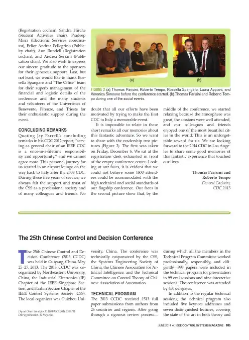
JUNE 2014 « IEEE CONTROL SYSTEMS MAGAZINE 105(Registration cochair), Sandra Hirche (Student Activities chair), Pradeep Misra (Electronic Services coordina-tor), Felice Andrea Pellegrino (Public-ity chair), Ann Rundell (Registration cochair), and Andrea Serrani (Publi-cation chair). We also wish to express our sincere gratitude to the sponsors for their generous support. L ast, but not least, we would like to thank Ros-sella Spangaro and “The Office” team for their superb management of the financial and logistic details of the conference and the many students and volunteers of the Universities of Benevento, Firenze, and Trieste for their enthusiastic support during the event.CONCLudING REMARkSQuoting Jay Farrell’s concluding remarks in his CDC 2012 report, “serv-ing as general chair of an IEEE CDC is a once-in-a-lifetime responsibil-ity and opportunity,” and we cannot agree more. This personal journey for us started in an airport lounge on the way back to Italy after the 2008 CDC. During these five years of service, we always felt the support and trust of the CSS as a professional society and of many colleagues and friends. Nodoubt that all our efforts have been motivated by trying to make the first CDC in Italy a memorable event.It is impossible to relate in these short remarks all our memories about this fantastic adventure. So we want to share with the readership two pic-tures (Figure 2). The first was taken on Friday, December 6. We sat at the registration desk exhausted in front of the empty conference center. Look-ing at our faces, it is evident that we could not believe some 1600 attend-ees could be accommodated with the high technical and social standards of our flagship conference. Our faces in the second picture show that, by themiddle of the conference, we started relaxing because the atmosphere was great, the sessions were well attended, and our colleagues and friends enjoyed one of the most beautiful cit-ies in the world. This is an unforget-table reward for us. We are looking forward to the 2014 CDC in Los Ange-les to share some good memories of this fantastic experience that touched our lives.Thomas Parisini andRoberto Tempo General Cochairs,CDC 2013(a)(b)FIGURE 2 (a) Thomas Parisini, Roberto Tempo, Rossella Spangaro, Laura Appiani, and Veronica Simeone before the conference started. (b) Thomas Parisini and Roberto Tem-po during one of the social events.The 25th Chinese Control and decision ConferenceDigital Object Identifier 10.1109/MCS.2014.2308731Date of publication: 12 May 2014The 25th Chinese Control and De-cision Conference (2013 CCDC) was held in Guiyang, China, May 25–27, 2013. The 2013 CCDC was co-organized by Northeastern University, China, the Industrial Electronics (IE) Chapter of the IEEE Singapore Sec-tion, and Harbin Section Chapter of the IEEE Control Systems Society (CSS). The local organizer was Guizhou Uni-versity, China. The conference was technically cosponsored by the CSS, the Systems Engineering Society of China, the Chinese Association for Ar-tificial Intelligence, and the Technical Committee on Control Theory of Chi-nese Association of Automation.TECHNICAL PROGRAMThe 2013 CCDC received 1513 full paper submissions from authors from 26 countries and regions. After going through a rigorous review process—during which all the members in the Technical Program Committee worked professionally, responsibly, and dili-gently—998 papers were included in the technical program for presentation in 99 oral sessions and nine interactive sessions. The conference was attended by 650 delegates.In addition to the regular technical sessions, the technical program also included five keynote addresses and seven distinguished lectures, covering the state of the art in both theory and106 IEEE CONTROL SYSTEMS MAGAZINE » JUNE 2014applications in control, decision, auto-mation, robotics, and emerging technol-ogies. The five keynote addresses were»“Perception-Enabled Control—A New Paradigm for Biomimet-ics and Machine Autonomy” by John Baillieul, Boston Univer-sity, United States»“Recursive Approach to System Identification” by Han-Fu Chen, Chinese Academy of Sciences, China»“Sc ience, Tec h nolog y a nd Industry, Quo Vadis?” by Okyay Kaynak, Bogazici University, Turkey»“Signal Processing via Sampled-data Control—Beyond Shan-non” by Yutaka Yamamoto, Kyoto University, Japan»“Hardware-in-Loop Simula-tion” by Zicai Wang, Harbin Institute of Technology, China.Distinguished lectures were delivered by Xiaohua Xia of the University of Pretoria, South Africa, “Applications of Model Predictive Control in Opera-tion Efficiency Optimization,” Ji-Feng Zhang of the Chinese Academy of Sciences, China, “How Much Infor-mation Is Needed for a Given Control Task,” Jagannathan Sarangapani of the Missouri University of Science and Technology, United States, “Optimal Adaptive Control of Uncertain Non-linear Dynamic Systems,” Jun Wang of The Chinese University of Hong Kong, China, “Neurodynamic OptimizationApproaches to Robust Pole Assign-ment,” Jie Chen of City University of Hong Kong, China, “When Is a Time-Delay System Stable and Stabilizable?,” Guoxiang Gu of Jiangnan University, China, “New Perspectives of Consen-sus Control for Multi-agent Systems,” and Jiafu Tang of Northeastern Univer-sity, China, “Weight Vehicle Routing Problems and Beam Search Combined Max-Min Ant System.”All keynote addresses, distin-guished lectures, oral sessions, and interactive sessions were well attended and produced active discussions. The conference banquet, which included entertainment, was held in the evening of May 26, 2013.A CD-ROM that contained all papers presented at the conference was provided to each registered del-egate. The official conference proceed-ings were published by IEEE and are included in IEEE Xplore .ZHANG SI-YING (CCdC)OuTSTANdING YOuTH AWARdThe Zhang Si-Ying (CCDC) Outstand-ing Youth Paper Award is in recogni-tion of Zhang Si-Ying’s highly regarded perseverance, character, and academic contribution. The award also aims to inspire, motivate, and encourage young scholars in their research. For apaper to be eligible for the award, the first author of the paper must not be older than 35 on the day of the award presentation at the conference. The award is 3000 RMB with a certificate.The Award Committee for the 2013 CCDC was composed of five members:Zhong-Ping Jiang, United States, John Baillieul, United States, Changyun Wen, Singapore, Xin He Xu, China, and Guang-Hong Yang, China.For the 2013 CCDC, 133 papers were selected for consideration for theZhang Si-Ying Outstanding Youth PaperJohn Baillieul delivering a keynote address.Han-Fu Chen delivering a keynote address.Opening ceremony of the 2013 CCDC.Okyay Kaynak delivering a keynote address.Yutaka Yamamoto during his keynote session.JUNE 2014 « IEEE CONTROL SYSTEMS MAGAZINE 107Award based on reviewers’ comments,nominations, and the evaluations of theTechnical Program Committee mem-bers. These papers were sent to famousexperts including some members of theInternational Advisory Committee forfurther evaluation. Based on their evalu-ations and recommendation, the Techni-cal Program Committee short-listed fivepapers as the finalists for the Award:»“Exponential Stability of a Cou-pled Heat-ODE System” by Dong-Xia Zhao and Jun-Min Wang, Beijing Institute of Technology»“Global Exponential Stability of Nonlinear Impulsive Discrete System with Time Delay” by Kexue Zhang and Xinzhi L iu, University of Waterloo»“Nonlinear Oscillations in TCPnetworks with Drop-Tail Buffers” by Nizar Malangadan, Haseen Rahman, and Gaurav Raina, Indian Institute of Technology»“Globally Adaptive Path Track-ing Control of Under-actuated Ships” by Wei Wang and Jiangsh-uai Huang, Tsinghua University »“Finite Time Containment Con-trol of Nonlinear Multiagent Networks” by Di Yu, Lijuan Bai, and Weijian Ren, Northeast Petroleum University.During the conference, all Award Committee members attended the oral presentations of the five finalist papers. Each member independently assessedtheir originality, technical quality, and written and oral presentations. On the basis of these assessments, the 2013 CCDC Zhang Si-Ying Outstanding Youth Paper Award was presented toWei Wang from Tsinghua University.The International Advisory Commit-tee Chair of 2013 CCDC, Si-Ying Zhang, presented certificates to all the finalists and presented the award with a certifi-cate to the winner during the banquet.THE 26TH CHINESE CONTROLANd dECISION CONFERENCEThe 26th CCDC (2014 CCDC) will be held in Changsha, China, May 31 to June 2, 2014. Keynote addresses will be deliv-ered by Alessandro Astolfi of Imperial College, United Kingdom, Daizhan Cheng of the Chinese Academy of Sci-ences, and Jay A. Farrell of University of California, Riverside, United States. The Organizing Committee will invite prominent researchers as well as dis-tinguished lecturers. Information about the 2014 CCDC will be consistently updated on the conference Web site: .Changyun Wen andZhong-Ping Jiang International TechnicalProgram ChairsA well-attended banquet.2013 CCDC award committee members and finalists of the Zhang Si-Ying Outstanding Youth Award.Ke Fang, who delivered the keynote ad-dress for Prof. Zicai Wang.。
Robust ControlRobust control is a field of engineering and mathematics that deals with the design and implementation of control systems that can effectively handle uncertainty and variations in the system being controlled. This is an important area of study because in real-world applications, systems are often subject to various disturbances and uncertainties that can affect their behavior. Robust control aims to ensure that the system remains stable and performs as desired despite these uncertainties. One perspective on robust control is from the standpoint of aerospace engineering. In the field of aerospace, robust control is crucial for ensuring the stability and performance of aircraft and spacecraft. These vehicles operate in highly uncertain and dynamic environments, and their control systems must be able to adapt to changing conditions while maintaining stability and safety. Robust control techniques such as H-infinity control and mu-synthesis have been widely used in aerospace applications to design control systems that can handle uncertainties in the aerodynamic properties of the vehicle, variations in the operating conditions, and disturbances such as gusts and turbulence. Another perspective on robust control comes from the field of robotics. In robotics, control systems must be able to handle uncertainties in the dynamics of the robot and variations in the environment in which it operates. Robust control techniques such as sliding mode control and adaptive control have been applied to develop robot control systems that can maintain stability and achieve desired performance in the presence of uncertainties. This is particularly important for applications such as autonomous vehicles, where the robot must be able to operate in diverse and changing environments. From a theoretical perspective, robust control is grounded in the field of control theory and optimization. The development of robust control techniques involves the use of mathematical tools such as linear matrix inequalities (LMIs), convex optimization, and frequency domain analysis. These tools are used to formulate and solve the robust control design problem, which involves finding a control law that ensures stability and performance for a given range of uncertainties. The theoretical aspects of robust control are often complex and require a deep understanding of mathematical concepts, making it a challenging but intellectually rewarding fieldof study. In the industrial automation and process control domain, robust control plays a critical role in ensuring the stability and performance of industrial processes. Many industrial processes are subject to uncertainties and disturbances, such as variations in the parameters of the process, external disturbances, and equipment faults. Robust control techniques such as model predictive control (MPC) and robust PID control have been applied to address these challenges and improve the performance of industrial processes. Robust control is essential for maintaining the safety, efficiency, and quality of industrial operations, makingit an integral part of modern industrial automation systems. One of the key challenges in robust control is the trade-off between performance and robustness. In many cases, increasing the robustness of a control system may come at the cost of reduced performance, and vice versa. For example, a control system that is designed to be highly robust to uncertainties may exhibit conservative behaviorand may not be able to achieve the desired level of performance. On the other hand, a control system that is optimized for performance may be sensitive touncertainties and disturbances, leading to instability or poor performance in the presence of such disturbances. Balancing the trade-off between performance and robustness is a fundamental challenge in robust control design, and it requires careful consideration of the specific requirements and constraints of the application. In conclusion, robust control is a critical area of study in engineering and mathematics, with applications in aerospace, robotics, industrial automation, and many other fields. It addresses the challenge of designing control systems that can handle uncertainties and variations in the system being controlled, ensuring stability and performance in the presence of disturbances. Robust control techniques have been developed and applied in diverse domains, and they continue to be an active area of research and development. The theoreticaland practical aspects of robust control present both challenges and opportunities for engineers and researchers, making it a fascinating and important field of study.。
Robust ControlRobust control is a field of engineering and mathematics that focuses on designing systems that can perform effectively in the presence of uncertaintiesand variations. This is especially important in applications where the environment or operating conditions are unpredictable, such as in aerospace, automotive, and industrial control systems. The goal of robust control is to ensure that the system can maintain stability and performance despite these uncertainties, providing a reliable and consistent operation. One of the key challenges inrobust control is dealing with the inherent uncertainties in system dynamics, external disturbances, and measurement noise. Traditional control design methods often assume perfect knowledge of the system and its operating conditions, which can lead to poor performance or even instability when these assumptions are violated. Robust control techniques, on the other hand, explicitly account for these uncertainties and aim to provide guarantees on the system's behavior underall possible scenarios. There are several approaches to robust control, each with its own strengths and weaknesses. One common technique is H-infinity control,which seeks to minimize the worst-case performance of the system while taking into account the uncertainties. This approach is particularly well-suited for systems with hard performance requirements and where there is a need to explicitlyquantify the trade-offs between performance and robustness. Another popular approach to robust control is mu-synthesis, which is based on the theory of structured singular value analysis. This method allows for the design ofcontrollers that explicitly account for the structured uncertainties in the system, such as parametric variations or unmodeled dynamics. By considering these uncertainties in the controller design, mu-synthesis can provide improved robustness compared to traditional methods. In addition to these techniques,there are also other robust control methods such as loop-shaping, gain-scheduling, and model predictive control, each with its own set of advantages and limitations. The choice of method depends on the specific requirements of the application, as well as the available knowledge of the system and its uncertainties. From a practical perspective, robust control has a wide range of applications in various industries. For example, in aerospace engineering, robust control is essential forensuring the stability and performance of aircraft and spacecraft in the presence of uncertain aerodynamic forces, atmospheric disturbances, and sensor noise. Similarly, in automotive systems, robust control is used to design vehiclestability and traction control systems that can operate effectively under varying road conditions and driver inputs. In industrial automation, robust control is critical for maintaining the performance of manufacturing processes and robotic systems in the presence of uncertainties such as variations in material properties, external disturbances, and wear and tear. By incorporating robust control techniques into the design of these systems, engineers can ensure reliable operation and consistent performance, even in challenging and unpredictable environments. Despite its many benefits, robust control also has its limitations and challenges. One of the main difficulties in robust control is the trade-off between performance and conservatism. Because robust control techniques aim to provide guarantees under all possible uncertainties, they often lead to conservative designs that sacrifice some performance in order to ensure stability and robustness. This can be particularly challenging in applications where high performance is critical, such as in high-speed control systems or precision motion control. Another challenge in robust control is the complexity of the design process. Unlike traditional control design, which often relies on analytical or empirical methods, robust control design typically involves complex mathematical optimization and analysis techniques. This can make the design process more time-consuming and resource-intensive, requiring specialized expertise andcomputational tools. In addition, robust control techniques often requireaccurate knowledge of the system and its uncertainties, which may not always be available in practice. For example, in many real-world applications, the exact dynamics of the system or the magnitude of the uncertainties may be unknown or difficult to quantify. This can make it challenging to apply robust control techniques effectively and may require additional efforts in system identification and uncertainty quantification. Despite these challenges, the benefits of robust control in terms of reliability, safety, and performance make it an important and valuable tool for engineers and researchers. By addressing the uncertainties and variations inherent in complex systems, robust control techniques can provide alevel of confidence and assurance that is essential for critical applications in aerospace, automotive, and industrial systems. In conclusion, robust control is a vital field of study with wide-ranging applications and significant impact on various industries. By addressing uncertainties and variations in system dynamics, robust control techniques provide a means to ensure reliable and consistent performance, even in challenging and unpredictable environments. While there are challenges and limitations associated with robust control, its benefits in terms of stability, performance, and reliability make it an essential tool for engineers and researchers working in complex and uncertain systems. As technology continues to advance and new challenges emerge, the development and application of robust control techniques will remain a critical area of research and innovation.。
Robust ControlRobust control is a field of control theory that deals with the design of controllers that can handle uncertainties and disturbances in the system. The goal of robust control is to ensure that the system remains stable and performs well even in the presence of uncertainties and disturbances. In this response, I will discuss the importance of robust control, the challenges associated with designing robust controllers, and some of the techniques used in robust control. Robust control is important because most real-world systems are subject to uncertainties and disturbances. These uncertainties can arise from various sources, such as changes in the environment, sensor noise, or modeling errors. If a controller is designed without considering these uncertainties, the system may become unstableor perform poorly. Robust control techniques ensure that the controller can handle these uncertainties and disturbances, leading to a more reliable and robust system. Designing robust controllers is challenging because uncertainties and disturbances can be difficult to model and quantify. In addition, the design of robustcontrollers often requires trade-offs between performance and robustness. For example, a controller that is very robust to uncertainties may not provide thebest performance, while a controller that provides optimal performance may not be robust enough to handle uncertainties. Therefore, designing a robust controller requires careful consideration of the trade-offs between performance and robustness. There are several techniques used in robust control. One of the most common techniques is H-infinity control, which is based on the H-infinity norm.The H-infinity norm is a measure of the maximum gain from disturbances to theoutput of the system. H-infinity control seeks to minimize this gain whileensuring that the system remains stable. Another technique used in robust controlis mu-synthesis, which is based on the mu-norm. The mu-norm is a measure of the worst-case gain from uncertainties to the output of the system. Mu-synthesis seeks to minimize this gain while ensuring that the system remains stable. In additionto these techniques, there are also several other approaches to robust control,such as sliding mode control, adaptive control, and nonlinear control. Slidingmode control is a technique that uses a discontinuous control law to force the system to follow a desired trajectory. Adaptive control is a technique thatadjusts the controller parameters in real-time based on the system's behavior. Nonlinear control is a technique that uses nonlinear models to design controllers that can handle nonlinearities in the system. Overall, robust control is acritical field of study in control theory. It ensures that controllers can handle uncertainties and disturbances, leading to more reliable and robust systems. However, designing robust controllers is challenging and requires careful consideration of the trade-offs between performance and robustness. There are several techniques used in robust control, including H-infinity control, mu-synthesis, sliding mode control, adaptive control, and nonlinear control. Each of these techniques has its own strengths and weaknesses, and the choice of technique depends on the specific requirements of the system.。
Robust ControlRobust control, within the realm of engineering and specifically in the domain of control theory, is a concept that holds paramount importance in ensuring the stability and performance of systems in the face of uncertainties and variations.It's a fascinating area that delves into the intricacies of designing control systems capable of withstanding unforeseen disturbances and fluctuations, makingit an indispensable tool in various fields such as aerospace, automotive, robotics, and more. At its core, robust control seeks to address the inherent uncertainties and variations present in real-world systems. Unlike traditional control methods that assume perfect knowledge of system dynamics and disturbances, robust control acknowledges the presence of uncertainties and aims to develop controllers thatcan effectively handle them. This is particularly crucial in applications where system parameters may vary over time, environmental conditions are unpredictable, or disturbances occur unexpectedly. One of the key perspectives in robust control is the notion of stability. In conventional control design, stability is typically analyzed under ideal conditions, neglecting the effects of uncertainties. However, in robust control, stability analysis takes into account the worst-case scenario, ensuring that the system remains stable even in the presence of the most adverse conditions. This is achieved through techniques such as μ (mu) synthesis and H-infinity control, which provide robust stability guarantees by optimizingcontroller performance across a range of possible uncertainties. Beyond stability, robust control also addresses the performance aspect of control systems. While stability ensures that the system remains bounded under all conditions, performance deals with how well the system tracks reference signals and rejects disturbances. Robust control techniques aim to strike a balance between stability and performance, ensuring that the system not only remains stable but alsoachieves satisfactory performance in the presence of uncertainties. Another important perspective in robust control is that of trade-offs. In the design of robust controllers, engineers often face trade-offs between various conflicting objectives such as stability, performance, and robustness. For example, increasing the robustness of a controller may come at the expense of performance, or vice versa. Balancing these trade-offs requires careful consideration of systemrequirements and constraints, as well as a deep understanding of the underlying dynamics and uncertainties. Moreover, robust control extends beyond the design phase to implementation and real-world deployment. In practice, robust controllers must be validated and tested extensively to ensure that they perform as expected under various operating conditions. This involves conducting simulation studies, hardware-in-the-loop testing, and field trials to evaluate the robustness and performance of the controller in realistic scenarios. Additionally, robust control algorithms may need to be adapted or retuned over time to accommodate changes in system dynamics or operating conditions. In conclusion, robust control represents a fundamental paradigm shift in control theory, offering a systematic approach to designing controllers that can effectively handle uncertainties and variations in real-world systems. By focusing on stability, performance, trade-offs, and practical implementation considerations, robust control enables engineers to develop control systems that are not only stable and reliable but also capable of delivering satisfactory performance in the face of uncertainties. As technology continues to advance and systems become increasingly complex, the importance of robust control will only continue to grow, making it an indispensable tool for engineers across various disciplines.。
Table of ContentsPreface .................................................................................................................................................................... x iii Organization ......................................................................................................................................................... x viii Program Committees ............................................................................................................................................ x ix Funding ................................................................................................................................................................. x xiii Invited Talks .......................................................................................................................................................... x xv Tutorial and Workshop Summaries ................................................................................................................. x xxiii The Role of Machine Learning in Business Optimization (1)Chid ApteFAB-MAP: Appearance-Based Place Recognition and Mapping using a Learned VisualVocabulary Model (3)Mark Cummins, Paul NewmanDiscriminative Latent Variable Models for Object Detection (11)Pedro Felzenszwalb, Ross Girshick, David McAllester, Deva RamananWeb-Scale Bayesian Click-Through rate Prediction for Sponsored Search Advertising inMicrosoft's Bing Search Engine (13)Thore Graepel, Joaquin Quiñonero Candela, Thomas Borchert, Ralf HerbrichMusic Plus One and Machine Learning (21)Christopher RaphaelClimbing the Tower of Babel: Unsupervised Multilingual Learning (29)Benjamin Snyder, Regina BarzilayDetecting Large-Scale System Problems by Mining Console Logs (37)Wei Xu, Ling Huang, Armando Fox, David Patterson, Michael I. JordanParticle Filtered MCMC-MLE with Connections to Contrastive Divergence (47)Arthur U. Asuncion, Qiang Liu, Alexander T. Ihler, Padhraic SmythSurrogating the surrogate: accelerating Gaussian-process-based global optimization with amixture cross-entropy algorithm (55)Remi Bardenet, Balazs KeglForgetting Counts : Constant Memory Inference for a Dependent Hierarchical Pitman-YorProcess (63)Nicholas Bartlett, David Pfau, Frank WoodRobust Formulations for Handling Uncertainty in Kernel Matrices (71)Sahely Bhadra, Sourangshu Bhattacharya, Chiranjib Bhattacharyya, Aharon Ben-talActive Learning for Networked Data (79)Mustafa Bilgic, Lilyana Mihalkova, Lise GetoorDistance dependent Chinese restaurant processes (87)David M. Blei, Peter FrazierCausal filter selection in microarray data (95)Gianluca Bontempi, Patrick E. MeyerLabel Ranking under Ambiguous Supervision for Learning Semantic Correspondences (103)Antoine Bordes, Nicolas Usunier, Jason WestonA Theoretical Analysis of Feature Pooling in Visual Recognition (111)Y-Lan Boureau, Jean Ponce, Yann LeCunMulti-agent Learning Experiments on Repeated Matrix Games (119)Bruno Bouzy, Marc MetivierLearning Tree Conditional Random Fields (127)Joseph K. Bradley, Carlos GuestrinFinding Planted Partitions in Nearly Linear Time using Arrested Spectral Clustering (135)Nader H. Bshouty, Philip M. LongFast boosting using adversarial bandits (143)Róbert Busa-Fekete, Balázs KéglModeling Transfer Learning in Human Categorization with the Hierarchical Dirichlet Process (151)Kevin R. Canini, Mikhail M. Shashkov, Thomas L. GriffithsTransfer Learning for Collective Link Prediction in Multiple Heterogenous Domains (159)Bin Cao, Nathan Nan Liu, Qiang YangThe Elastic Embedding Algorithm for Dimensionality Reduction (167)Miguel Á. Carreira-PerpiñánRandom Spanning Trees and the Prediction of Weighted Graphs (175)Nicolo Cesa-Bianchi, Claudio Gentile, Fabio Vitale, Giovanni ZappellaEfficient Learning with Partially Observed Attributes (183)Nicolo Cesa-Bianchi, Shai Shalev-Shwartz, Ohad ShamirConvergence, Targeted Optimality, and Safety in Multiagent Learning (191)Doran Chakraborty, Peter StoneStructured Output Learning with Indirect Supervision (199)Ming-Wei Chang, Vivek Srikumar, Dan Goldwasser, Dan RothDynamical Products of Experts for Modeling Financial Time Series (207)Yutian Chen, Max WellingLabel Ranking Methods based on the Plackett-Luce Model (215)Weiwei Cheng, Krzysztof Dembczynski, Eyke HüllermeierGraded Multilabel Classification: The Ordinal Case (223)Weiwei Cheng, Krzysztof Dembczynski, Eyke HüllermeierComparing Clusterings in Space (231)Michael H. Coen, M. Hidayath Ansari, Nathanael FillmoreTwo-Stage Learning Kernel Algorithms (239)Corinna Cortes, Mehryar Mohri, Afshin RostamizadehGeneralization Bounds for Learning Kernels (247)Corinna Cortes, Mehryar Mohri, Afshin RostamizadehFast Neighborhood Subgraph Pairwise Distance Kernel (255)Fabrizio Costa, Kurt De GraveMining Clustering Dimensions (263)Sajib Dasgupta, Vincent NgBottom-Up Learning of Markov Network Structure (271)Jesse Davis, Pedro DomingosBayes Optimal Multilabel Classification via Probabilistic Classifier Chains (279)Krzysztof Dembczynski, Weiwei Cheng, Eyke HüllermeierA Conditional Random Field for Multiple-Instance Learning (287)Thomas Deselaers, Vittorio FerrariAsymptotic Analysis of Generative Semi-Supervised Learning (295)Joshua V. Dillon, Krishnakumar Balasubramanian, Guy LebanonHeterogeneous Continuous Dynamic Bayesian Networks with Flexible Structure and Inter-TimeSegment Information Sharing (303)Frank Dondelinger, Sophie Lebre, Dirk HusmeierTemporal Difference Bayesian Model Averaging:A Bayesian Perspective on Adapting Lambda (311)Carlton Downey, Scott SannerHigh-Performance Semi-Supervised Learning using Discriminatively Constrained GenerativeModels (319)Gregory Druck, Andrew McCallumOn the Consistency of Ranking Algorithms (327)John C. Duchi, Lester W. Mackey, Michael I. JordanInverse Optimal Control with Linearly-Solvable MDPs (335)Krishnamurthy Dvijotham, Emanuel TodorovContinuous-Time Belief Propagation (343)Tal El-Hay, Ido Cohn, Nir Friedman, Raz KupfermanNonparametric Information Theoretic Clustering Algorithm (351)Lev Faivishevsky, Jacob GoldbergerFeature Selection as a One-Player Game (359)Romaric Gaudel, Michele SebagMultiscale Wavelets on Trees, Graphs and High Dimensional Data: Theory and Applications toSemi Supervised Learning (367)Matan Gavish, Boaz Nadler, Ronald R. CoifmanA Language-based Approach to Measuring Scholarly Impact (375)Sean M. Gerrish, David M. BleiBoosting Classifiers with Tightened L0-Relaxation Penalties (383)Noam Goldberg, Jonathan EcksteinBudgeted Nonparametric Learning from Data Streams (391)Ryan Gomes, Andreas KrauseLearning Fast Approximations of Sparse Coding (399)Karol Gregor, Yann LeCunBoosted Backpropagation Learning for Training Deep Modular Networks (407)Alexander Grubb, J. Andrew BagnellInteractive Submodular Set Cover (415)Andrew Guillory, Jeff BilmesLarge Scale Max-Margin Multi-Label Classification with Priors (423)Bharath Hariharan, Lihi Zelnik-Manor, S. V. N. Vishwanathan, Manik VarmaActive Learning for Multi-Task Adaptive Filtering (431)Abhay Harpale, Yiming YangBayesian Nonparametric Matrix Factorization for Recorded Music (439)Matthew D. Hoffman, David M. Blei, Perry R. CookMulti-Task Learning of Gaussian Graphical Models (447)Jean Honorio, Dimitris SamarasLearning Hierarchical Riffle Independent Groupings from Rankings (455)Jonathan Huang, Carlos GuestrinOn learning with kernels for unordered pairs (463)Martial Hue, Jean-Philippe VertA Simple Algorithm for Nuclear Norm Regularized Problems (471)Martin Jaggi, Marek SulovskýTelling cause from effect based on high-dimensional observations (479)Dominik Janzing, Patrik O. Hoyer, Bernhard SchölkopfProximal Methods for Sparse Hierarchical Dictionary Learning (487)Rodolphe Jenatton, Julien Mairal, Guillaume Obozinski, Francis Bach3D Convolutional Neural Networks for Human Action Recognition (495)Shuiwang Ji, Wei Xu, Ming Yang, Kai YuAccelerated dual decomposition for MAP inference (503)Vladimir Jojic, Stephen Gould, Daphne KollerEfficient Selection of Multiple Bandit Arms: Theory and Practice (511)Shivaram Kalyanakrishnan, Peter StoneA scalable trust-region algorithm with application to mixed-norm regression (519)Dongmin Kim, Suvrit Sra, Inderjit DhillonLocal Minima Embedding (527)Minyoung Kim, Fernando De la TorreGaussian Processes Multiple Instance Learning (535)Minyoung Kim, Fernando De la TorreTree-Guided Group Lasso for Multi-Task Regression with Structured Sparsity (543)Seyoung Kim, Eric P. XingLearning Markov Logic Networks Using Structural Motifs (551)Stanley Kok, Pedro DomingosOn Sparse Nonparametric Conditional Covariance Selection (559)Mladen Kolar, Ankur P. Parikh, Eric P. XingSubmodular Dictionary Selection for Sparse Representation (567)Andreas Krause, Volkan CevherImplicit Online Learning (575)Brian Kulis, Peter L. BartlettProbabilistic Backward and Forward Reasoning in Stochastic Relational Worlds (583)Tobias Lang, Marc ToussaintSupervised Aggregation of Classifiers using Artificial Prediction Markets (591)Nathan Lay, Adrian BarbuBayesian Multi-Task Reinforcement Learning (599)Alessandro Lazaric, Mohammad GhavamzadehAnalysis of a Classification-based Policy Iteration Algorithm (607)Alessandro Lazaric, Mohammad Ghavamzadeh, Rémi MunosFinite-Sample Analysis of LSTD (615)Alessandro Lazaric, Mohammad Ghavamzadeh, Rémi MunosA fast natural Newton method (623)Nicolas Le Roux, Andrew FitzgibbonMaking Large-Scale Nystr•om Approximation Possible (631)Mu Li, James T. Kwok, Bao-Liang LuLearning Programs: A Hierarchical Bayesian Approach (639)Percy Liang, Michael I. Jordan, Dan KleinOn the Interaction between Norm and Dimensionality: Multiple Regimes in Learning (647)Percy Liang, Nati SrebroPower Iteration Clustering (655)Frank Lin, William W. CohenRobust Subspace Segmentation by Low-Rank Representation (663)Guangcan Liu, Zhouchen Lin, Yong YuRobust Graph Mode Seeking by Graph Shift (671)Hairong Liu, Shuicheng YanLarge Graph Construction for Scalable Semi-Supervised Learning (679)Wei Liu, Junfeng He, Shih-Fu ChangLearning Temporal Causal Graphs for Relational Time-Series Analysis (687)Yan Liu, Alexandru Niculescu-Mizil, Aurélie Lozano , Yong LuEfficient Reinforcement Learning with Multiple Reward Functions for Randomized ControlledTrial Analysis (695)Daniel J. Lizotte, Michael Bowling, Susan A. MurphyRestricted Boltzmann Machines are Hard to Approximately Evaluate or Simulate (703)Philip M. Long, Rocco A. ServedioMixed Membership Matrix Factorization (711)Lester Mackey, David Weiss, Michael I. JordanToward Off-Policy Learning Control with Function Approximation (719)Hamid Reza Maei, Csaba Szepesvari, Shalabh Bhatnagar, Richard S. SuttonConstructing States for Reinforcement Learning (727)M. M. Hassan MahmudDeep learning via Hessian-free optimization (735)James MartensLearning the Linear Dynamical System with ASOS (743)James MartensFrom Transformation-Based Dimensionality Reduction to Feature Selection (751)Mahdokht Masaeli, Glenn Fung, Jennifer G. DyRisk minimization, probability elicitation, and cost-sensitive SVMs (759)Hamed Masnadi-Shirazi, Nuno VasconcelosExploiting Data-Independence for Fast Belief-Propagation (767)Julian J. McAuley, Tibério S. CaetanoMetric Learning to Rank (775)Brian McFee, Gert LanckrietLearning Efficiently with Approximate Inference via Dual Losses (783)Ofer Meshi, David Sontag, Tommi Jaakkola, Amir GlobersonDeep Supervised t-Distributed Embedding (791)Renqiang Min, Laurens van der Maaten, Zineng Yuan, Anthony Bonner, Zhaolei ZhangNonparametric Return Distribution Approximation for Reinforcement Learning (799)Tetsuro Morimura, Masashi Sugiyama, Hisashi Kashima , Hirotaka Hachiya, Toshiyuki TanakaRectified Linear Units Improve Restricted Boltzmann Machines (807)Vinod Nair, Geoffrey E. HintonImplicit Regularization in Variational Bayesian Matrix Factorization (815)Shinichi Nakajima, Masashi SugiyamaEstimation of (near) low-rank matrices with noise and high-dimensional scaling (823)Sahand Negahban, Martin J. WainwrightMultiple Non-Redundant Spectral Clustering Views (831)Donglin Niu, Jennifer G. Dy, Michael I. JordanMultiagent Inductive Learning: an Argumentation-based Approach (839)Santiago Ontañón, Enric PlazaA Stick-Breaking Construction of the Beta Process (847)John Paisley, Aimee Zaas, Christopher W. Woods, Geoffrey S. Ginsburg, Lawrence CarinThe Margin Perceptron with Unlearning (855)Constantinos Panagiotakopoulos, Petroula TsampoukaBoosting for Regression Transfer (863)David Pardoe, Peter StoneFeature Selection Using Regularization in Approximate Linear Programs for Markov DecisionProcesses (871)Marek Petrik, Gavin Taylor, Ron Parr, Shlomo Zilberstein*Budgeted Distribution Learning of Belief Net Parameters (879)Liuyang Li, Barnabás Póczos, Csaba Szepesvári, Russ GreinerVariable Selection in Model-Based Clustering: To Do or To Facilitate (887)Leonard K. M. Poon, Nevin L. Zhang, Tao Chen, Yi WangApproximate Predictive Representations of Partially Observable Systems (895)Monica Dinculescu, Doina PrecupSpherical Topic Models (903)Joseph Reisinger, AustinWaters, Bryan Silverthorn, Raymond J. MooneySVM Classifier Estimation from Group Probabilities (911)Stefan RuepingClustering processes (919)Daniil RyabkoGaussian Process Change Point Models (927)Yunus Saatçi, Ryan Turner, Carl Edward RasmussenOnline Prediction with Privacy (935)Jun Sakuma, Hiromi AraiLearning Deep Boltzmann Machines using Adaptive MCMC (943)Ruslan SalakhutdinovActive Risk Estimation (951)Christoph Sawade , Niels Landwehr, Steffen Bickel, Tobias SchefferShould one compute the Temporal Difference fix point or minimize the Bellman Residual ? Theunified oblique projection view (959)Bruno ScherrerGaussian Covariance and Scalable Variational Inference (967)Matthias W. SeegerApplication of Machine Learning To Epileptic Seizure Detection (975)Ali Shoeb, John GuttagLearning optimally diverse rankings over large document collections (983)Aleksandrs Slivkins, Filip Radlinski, Sreenivas GollapudiHilbert Space Embeddings of Hidden Markov Models (991)Le Song, Sajid M. Siddiqi, Geoffrey Gordon, Alex SmolaCOFFIN : A Computational Framework for Linear SVMs (999)Soeren Sonnenburg, Vojtech FrancInternal Rewards Mitigate Agent Boundedness (1007)Jonathan Sorg, Satinder Singh, Richard LewisGaussian Process Optimization in the Bandit Setting: No Regret and Experimental Design (1015)Niranjan Srinivas, Andreas Krause, Sham Kakade, Matthias SeegerUnsupervised Risk Strati cation in Clinical Datasets: Identifying Patients at Risk of RareOutcomes (1023)Zeeshan Syed, Ilan RubinfeldModel-based reinforcement learning with nearly tight exploration complexity bounds (1031)István Szita, Csaba SzepesváriTotal Variation and Cheeger Cuts (1039)Arthur Szlam, Xavier BressonLearning Sparse SVM for Feature Selection on Very High Dimensional Datasets (1047)Mingkui Tan, Li Wang, Ivor W. TsangDeep networks for robust visual recognition (1055)Yichuan Tang, Chris EliasmithA DC Programming Approach for Sparse Eigenvalue Problem (1063)Mamadou Thiao, Tao Pham Dinh, Hoai An Le ThiLeast-Squares Policy Iteration: Bias-Variance Trade-off in Control Problems (1071)Christophe Thiery, Bruno ScherrerAn Analysis of the Convergence of Graph Laplacians (1079)Daniel Ting, Ling Huang, Michael I. JordanA Fast Augmented Lagrangian Algorithm for Learning Low-Rank Matrices (1087)Ryota Tomioka, Taiji Suzuki, Masashi Sugiyama, Hisashi KashimaOne-sided Support Vector Regression for Multiclass Cost-sensitive Classification (1095)Han-Hsing Tu, Hsuan-Tien LinNon-Local Contrastive Objectives (1103)David Vickrey, Cliff Chiung-Yu Lin, Daphne KollerThe Translation-invariant Wishart-Dirichlet Process for Clustering Distance Data (1111)Julia E. Vogt, Sandhya Prabhakaran, Thomas J. Fuchs, Volker RothGeneralizing Apprenticeship Learning across Hypothesis Classes (1119)Thomas J. Walsh, Kaushik Subramanian, Michael L. Littman, Carlos DiukSequential Projection Learning for Hashing with Compact Codes (1127)Jun Wang, Sanjiv Kumar, Shih-Fu ChangA New Analysis of Co-Training (1135)Wei Wang, Zhi-Hua ZhouMulti-Class Pegasos on a Budget (1143)Zhuang Wang, Koby Crammer, Slobodan VuceticThe IBP Compound Dirichlet Process and its Application to Focused Topic Modeling (1151)Sinead Williamson, Chong Wang, Katherine A. Heller, David M. BleiOnline Streaming Feature Selection (1159)Xindong Wu, Kui Yu, Hao Wang, Wei DingClasses of Multiagent Q-learning Dynamics with -greedy Exploration (1167)Michael Wunder, Michael Littman, Monica BabesSimple and Efficient Multiple Kernel Learning by Group Lasso (1175)Zenglin Xu, Rong Jin, Haiqin Yang, Irwin King, Michael R. LyuSparse Gaussian Process Regression via l1 Penalization (1183)Feng Yan, Yuan (Alan) QiOnline Learning for Group Lasso (1191)Haiqin Yang, Zenglin Xu, Irwin King, Michael R. LyuLearning from Noisy Side Information by Generalized Maximum Entropy Model (1199)Tianbao Yang, Rong Jin, Anil K. JainConvergence of Least Squares Temporal Difference Methods Under General Conditions (1207)Huizhen YuImproved Local Coordinate Coding using Local Tangents (1215)Kai Yu, Tong ZhangProjection Penalties: Dimension Reduction without Loss (1223)Yi Zhang, Jeff SchneiderOTL: A Framework of Online Transfer Learning (1231)Peilin Zhao, Steven C.H. HoiConditional Topic Random Fields (1239)Jun Zhu, Eric P. XingCognitive Models of Test-Item Effects in Human Category Learning (1247)Xiaojin Zhu, Bryan R. Gibson, Kwang-Sung Jun, Timothy T. Rogers, Joseph Harrison, Chuck KalishModeling Interaction via the Principle of Maximum Causal Entropy (1255)Brian D. Ziebart, J. Andrew Bagnell, Anind K. Dey。
Robust ControlRobust control is a field of engineering that deals with the design and implementation of control systems that are able to perform reliably in the presence of uncertainties and disturbances. It is an essential aspect of modern engineering, as it ensures that control systems can operate effectively even in the face of unpredictable factors. One perspective on robust control is from the standpoint of an engineer designing a control system. From this perspective, the goal is to create a control system that can handle a wide range of uncertainties and disturbances. This requires a deep understanding of the system being controlled, as well as the ability to model and predict the effects of uncertainties and disturbances. To achieve robust control, engineers utilize various techniques and tools. One common approach is to use feedback control, where the output of the system is measured and compared to a desired reference value. Any difference between the measured output and the reference value is used to adjust the control inputs in order to minimize the error. This feedback loop helps to compensate for uncertainties and disturbances, ensuring that the system remains stable and performs as desired. Another important aspect of robustcontrol is the use of robust design methods. These methods involve designing the control system to be inherently robust to uncertainties and disturbances. This can be achieved through techniques such as loop shaping, where the frequency response of the control system is modified to ensure stability and performance in the presence of uncertainties. From the perspective of a system being controlled, robust control can provide numerous benefits. For example, in a manufacturing process, robust control can help to ensure that the process operates consistently and produces high-quality products, even in the presence of variations in raw materials or operating conditions. Similarly, in a flight control system, robust control can help to ensure the stability and safety of the aircraft, even in the face of unpredictable weather conditions or system failures. Robust control also has implications for society as a whole. For example, in the field of autonomous vehicles, robust control is crucial to ensure the safety and reliability of these vehicles. By designing control systems that can handle uncertainties and disturbances, engineers can help to prevent accidents and improve the overallefficiency of transportation systems. In conclusion, robust control is a vital aspect of modern engineering. It allows control systems to operate effectively in the presence of uncertainties and disturbances, ensuring stability, performance, and safety. From the perspective of an engineer, robust control involves designing control systems that can handle a wide range of uncertainties and disturbances. This requires a deep understanding of the system being controlled and the use of techniques such as feedback control and robust design methods. From the perspective of a system being controlled, robust control provides numerous benefits, including consistent operation and high-quality output. In society as a whole, robust control has implications for safety, reliability, and efficiency in various domains, such as manufacturing and transportation.。
Robust ControlRobust control is a critical concept in the field of engineering and automation. It refers to the ability of a control system to maintain stability and performance in the presence of uncertainties and variations in the system being controlled. This is particularly important in real-world applications where environmental factors, component variations, and external disturbances can all impact the behavior of the system. One perspective on robust control is from the standpoint of system design and analysis. Engineers and researchers in this field are tasked with developing control algorithms and strategies that can effectively handle uncertainties and variations in the system. This often involves the use of mathematical models, simulation tools, and advanced control techniques to ensure that the system remains stable and performs as expected under a wide range of operating conditions. From a practical standpoint, robust control is essentialfor ensuring the reliable and safe operation of complex systems. For example, in aerospace engineering, robust control techniques are used to design flight control systems that can handle variations in aircraft dynamics, atmospheric disturbances, and sensor noise. Similarly, in industrial automation, robust control is necessary for maintaining the performance of manufacturing processes in the face of changing operating conditions and disturbances. Another perspective on robust control is the impact it has on the end-users of the controlled systems. For example, in the automotive industry, robust control is crucial for ensuring the safety and comfort of vehicle occupants. Control systems that can effectively handle uncertainties in road conditions, vehicle dynamics, and external disturbances are essential for providing a smooth and predictable driving experience. From an economic standpoint, robust control can have significant implications for the cost and performance of engineered systems. For example, in the energy sector, robust control techniques are used to optimize the performance of power generation and distribution systems while ensuring the stability and reliability of the grid. By minimizing the impact of uncertainties and disturbances, robust control can help to reduce maintenance costs, improve energy efficiency, and enhance overall system performance. In conclusion, robust control is a critical concept in engineering and automation, with implications for system design, practical applications, end-user experience, and economic considerations. By addressing uncertainties and variations in the system, robust control techniques play a crucial role in ensuring the stability, reliability, and performance of complex engineered systems in a wide range of industries. As technology continues to advance and systems become increasingly complex, the importance of robust control will only continue to grow, making it a key area of focus for engineers and researchers around the world.。
Robust Control and Estimation Robust control and estimation is a field of study within control systems engineering that deals with designing control systems that are able to handle uncertainties and disturbances. It is an important area of research as many real-world systems are subject to uncertainties and disturbances, such as noise, parameter variations, and external disturbances. In this response, I will discuss the importance of robust control and estimation from multiple perspectives. From an engineering perspective, robust control and estimation techniques are crucialfor ensuring the stability and performance of control systems in the presence of uncertainties. Traditional control techniques, such as PID controllers, are designed based on accurate mathematical models of the system. However, in practice, these models are often not perfect and uncertainties exist. Robust control techniques, such as H-infinity control and mu-synthesis, provide a framework for designing controllers that can handle these uncertainties and guarantee certain performance specifications. By considering the worst-case scenario, robust control techniques provide a level of confidence in the control system's ability tooperate under uncertain conditions. From a practical perspective, robust control and estimation techniques are essential for dealing with real-world challenges.For example, in autonomous vehicles, uncertainties in the road conditions, vehicle dynamics, and sensor measurements can significantly affect the performance and safety of the vehicle. Robust control and estimation techniques can help mitigate these uncertainties and ensure stable and reliable autonomous operation. Similarly, in aerospace applications, uncertainties in the aircraft dynamics, environmental conditions, and sensor measurements can have a significant impact on the flight control system. Robust control and estimation techniques are used to design flight control systems that can handle these uncertainties and guarantee safe andefficient flight. From a business perspective, robust control and estimation techniques can have a significant impact on the bottom line. By improving the performance and stability of control systems, robust control techniques can leadto increased productivity, reduced downtime, and improved product quality. For example, in manufacturing processes, uncertainties in the process parameters can lead to variations in product quality. Robust control techniques can help minimizethese variations and improve the overall product quality. Similarly, in power systems, uncertainties in the demand and generation can lead to instability and blackouts. Robust control techniques can help ensure the stability and reliability of the power system, leading to cost savings and improved customer satisfaction. From a societal perspective, robust control and estimation techniques are important for ensuring the safety and well-being of individuals. In critical applications, such as medical devices and nuclear power plants, uncertainties in the system dynamics can have severe consequences. Robust control techniques are used to design control systems that can handle these uncertainties and ensure safe operation. Similarly, in environmental monitoring and control, uncertainties in the environmental conditions can have a significant impact on the ecosystem. Robust control techniques can help mitigate these uncertainties and ensure the preservation of the environment. In conclusion, robust control and estimation techniques play a crucial role in control systems engineering from multiple perspectives. From an engineering perspective, they provide a framework for designing control systems that can handle uncertainties and disturbances. From a practical perspective, they are essential for dealing with real-world challenges in various applications. From a business perspective, they can have a significant impact on productivity, quality, and cost savings. From a societal perspective, they are important for ensuring safety and well-being. Overall, robust control and estimation techniques are a vital area of research that continues to evolve and contribute to the advancement of control systems engineering.。
1automation 自动化1closed-loop 闭环1open-loop 开环1feedback反馈1closed-loop feedback control system 闭环反馈控制系统1open-loop control system 开环控制系统1negative feedback 负反馈1positive feedback 正反馈1control system控制系统1complexity of design 设计复杂性1design 设计1design gap设计差距1engineering design 工程设计1feedback signal 反馈信号1flyball governor飞球调节器1multivariable control system 多变量控制系统1optimization 优化1plant 对象1process过程1productivity 生产率1risk 风险1robot机器人1specifications 指标说明1synthesis 综合1system 系统1trade-off折中2actuator 执行机构/执行器2assumptions 假设条件2block diagrams框图2characteristic equation 特征方程2transfer function 传递函数2closed-loop transfer function 闭环传递函数2open-loop transfer function 开环传递函数2damping阻尼2damping ratio 阻尼系数/阻尼比2critical damping 临界阻尼2damping oscillation 阻尼振荡2DC motor直流电机2differential equation 微分方程2error误差2error signal 误差信号2final value终值2final value theorem 终值定理2homogeneity齐次性2Laplace transform 拉普拉斯变换2linear approximation 线性近似2linear system线性系统2linearized线性化的chterm translation2linearization线性化2Mason loop rule梅森回路规则2Mason formula梅森公式2natural frequency固有频率/自然频率2necessary condition必要条件2overdamped过阻尼的2poles极点2zeros零点2principle of superposition叠加原理2reference input参考输入2residues留数2signal-flow graph信号流图2simulation 仿真2steady state稳态2s-plane s平面2Taylor series泰勒级数2time constant时间常数2underdamped欠阻尼的2unity feedback单位反馈3canonical form标准型3diagonal canonical form对角标准型/对角线标准型3discrete-time approximation离散时间近似3Euler's method欧拉方法3fundamental matrix基本矩阵3input feedforward canonical form输入前馈标准型3Jordan canonical form约当标准型3matrix exponential function矩阵指数函数3output equation输出方程3phase variable canonical form相变量标准型3phase variable相变量3physical variables物理变量3state differential equation状态微分方程3state space状态空间3state variables状态变量3state vector状态向量/状态矢量3state of a system系统状态3state-space representation状态空间表示/状态空间表达式3state variable feedback状态变量反馈3time domain时域3time-varying system时变系统3time-invariant system时不变系统/非时变系统3transition matrix转移矩阵4closed-loop system闭环系统4complexity复杂度4components组件4direct system直接系统4disturbance signal扰动信号4error signal误差信号4instability不稳定性4loss of gain增益损失4open-loop system开环系统4steady-state error稳态误差4system sensitivity系统灵敏度4transient response暂态响应/瞬态响应4steady-state response稳态响应5acceleration error constant,Ka加速度误差常数,Ka5position error constant,Kp位置误差常数,Kp5velocity error constant,Kv速度误差常数,Kv5design specifications设计要求5domainant roots主导极点5optimum control system最优控制系统5peak time峰值时间5percent overshoot百分比超调/超调量5maximum percent overshoot最大超调量5performance index性能指标5rise time 上升时间5settling time 调整时间5test input signal测试输入信号5tyoe number型数5unit impulse单位脉冲6absolute stability绝对稳定性6auxiliary polynomial辅助多项式6marginally stable临界稳定6relative stability相对稳定性6Rooth-Hurwitz criterion Rooth-Hurwitz判据/劳斯-赫尔维茨判据6stability稳定性6stable system稳定系统7angle of departure出射角7angle of the asymptotes渐近角7asymptote渐近线7asymptote centroid渐近中心7breakaway point分支点7dominant roots主导极点7locus轨迹7logarithmic sensitivity对数灵敏度7number of separate loci根轨迹的段数7parameter design参数设计7PID controller PID控制器7proportional plus derivative (PD) controller比例加微分(PD)控制器7proportional plus integral (PI) controller比例加积分(PI)控制器7root contours根等值线7root locus根轨迹7root locus method根轨迹法7root locus segments on the real axis实轴上的根轨迹段7root sensitivity根灵敏度8all-pass network全通网络8bandwidth带宽8Bode plot Bode图/波德图8break frequency截止频率8corner frequency转折频率8decade十倍频程8Decibel/dB分贝8Fourier transform Fourier变换/傅里叶变换8Fourier transform pair Fourier变换对/傅里叶变换对8frequency response频率响应8Laplace transform pair拉普拉斯变换对8Logarithmic magnitude对数幅值8Logarithmic plot对数坐标图8maximum value of the frequency response频率响应的最大值8minimum phase transfer dunction最小相位传递函数8nonminimum phase system非最小相位系统8polar plot极坐标图8resonant frequency谐振频率8transfer function in the frequency domain频域传递函数9Cauchy's theorem Cauchy定理9closed-loop frequency response闭环频率响应9conformal mapping保角映射9contour map围道映射9gain margin增益裕度/增益裕量9logarithmic (decibel) measure对数(分贝)度量9Nichols chart Nichols图9Nyquist stability criterion Nyquist稳定判据/奈奎斯特稳定判据9phase margin相角裕度/相位裕度9principle of the argument幅角原理9time delay时滞10cascade compensation network串联校正网络10compensation校正10compensator校正装置10deadbeat response最小拍响应10design of a control system控制系统设计10integration network积分网络10lag network滞后网络10lead network超前网络10lead-lag network超前滞后网络10phase lag compensation相角滞后校正10phase lead compensation相角超前校正10phase-lag network相角滞后网络10phase-lead network相角超前网络10prefilter前置滤波11command following给定跟踪11controllability matrix能控性矩阵11controllable system能控系统11detectable能检测11estimation error估计误差11full-state feedback control law全状态反馈控制律11internal mode design内模设计11Kalman state-space decomposition Kalman状态空间分解/卡尔曼状态空间分解11linear quadratic regulator线性二次型调节器11observable system能观系统11observability matrix能观性矩阵11observer观测器11optimal control system最优控制系统11pole assignment极点配置11separation principle分离原理11stabilizable能镇定11stabilizing controller镇定控制器11state variable feedback状态变量反馈12additive perturbation加性摄动12complementary sensitivity function补灵敏度函数12internal model principle内模原理12mulplicative perturbation乘性摄动12process controller过程控制器12robust control system鲁棒控制系统12robust stability criterion鲁棒稳定判据12root sensitivity根灵敏度12system sensitivity系统灵敏度12three-mode controller三模态控制器12three-term controller三项控制器13amplitude quantization error幅值量化误差13backward difference rule后向差分规则13digital computer compensator数字计算机校正装置13digital controll system数字控制系统13forward rectangular integration前向矩形积分13microcomputer微型计算机13minicomputer小型计算机13digital PID controller数字PID控制器13precision精度13sampled data采样数据13sampled-data system采样数据系统13sampling period采样周期13stability of sampled-data system采样数据系统的稳定性13z-plane z平面13z-transform z变换13zero-order hold零阶保持13zero-order holder零阶保持器。
第 23卷第 1期2024年 1月Vol.23 No.1Jan.2024软件导刊Software Guide基于贝叶斯理论的HotellingT2小样本多元工序质量监控方法宁方华1,骞文成1,屠震元2,陈智峰1(1.浙江理工大学机械工程学院,浙江杭州 310018;2.杭州海康威视数字技术股份有限公司,浙江杭州 310051)摘要:适用于多元质量控制的传统HotellingT2控制图方法,在小批量加工时因样本数据少而对异常值较敏感,存在一定局限性。
为此,将贝叶斯理论与传统HotellingT2控制图相结合,通过历史批次工序质量分布信息和现有样本实时数据估计贝叶斯参数,构造基于贝叶斯理论的HotellingT2工序质量控制图,以在小批量加工的多元质量控制过程中抵御异常值造成的影响。
通过发动机凸轮轴工序质量控制实例分析表明,所提方法相较于传统方法能有效抵御异常值造成的影响,具有良好的抗干扰性和稳定性,能更好地监测工序质量控制的失控状态。
关键词:多元质量控制;贝叶斯理论;HotellingT2控制图DOI:10.11907/rjdk.222482开放科学(资源服务)标识码(OSID):中图分类号:TP183 文献标识码:A文章编号:1672-7800(2024)001-0122-06HotellingT2 Small Sample Multivariate Process Quality Monitoring MethodBased on Bayesian TheoryNING Fanghua1, QIAN Wencheng1, TU Zhenyuan2, CHEN Zhifeng1(1.School of Mechanical Engineering, Zhejiang Sci-tech University, Hangzhou 310018, China;2.Hangzhou Hikvision DIGITAL Technology Co., Ltd., Hangzhou 310051, China)Abstract:Traditional Hotelling T2 control chart method suitable for multivariate quality control has certain limitations in small batch process⁃ing due to its sensitivity to outliers due to limited sample data. To this end, Bayesian theory is combined with traditional Hotelling T2 control charts to estimate Bayesian parameters through historical batch process quality distribution information and existing real-time sample data. A Hotelling T2 process quality control chart based on Bayesian theory is constructed to resist the impact of outliers in the multivariate quality con⁃trol process of small batch processing. The analysis of quality control examples for engine camshaft processes shows that the proposed method can effectively resist the impact of outliers compared to traditional methods, has good anti-interference and stability, and can better monitor the uncontrolled state of process quality control.Key Words:multivariate quality control; Bayesian theory; HotellingT2 control chart0 引言在生产加工过程中,为了保证产品质量需要同时监控每个方面的质量指标。
Data Mining 数据挖掘技术例句:We hope to answer all of your initial questions about data mining .我们希望能够回答您所有关于数据挖掘的初级问题。
subject-oriented 面向主题的例 A data warehouse is a, by definition, subject-oriented , integrated,non -volatile and time -variant repository of data to support decision for manager.数据仓库是一个面向主题的、集成的、相对稳固的且随时光不断变化的数据聚集,用来支持管理人员的决议计划。
integrated 集成的例句:Does not test for integration issues: The security of a system requiresthat all of the system components be secure when integrated with each other. 不能测试整合问题:一个系统的安全性需要在与其它控件整合时保证这个系统的所有控件都是安全的。
time-variant 实时的例句:Classic PID control method which is based on precise mathematical model has poor adaptivity and is not adaptive to nonlinear and time-variant plants.经典的基于对象精确数学模型的PID 控制方法的自适应性较差,难以适应具有非线性、时变不确定性的被控对象。
nonvolatile 非已失的例句:Valuable data assets reside in nonvolatile memory so they are protected against the loss of electrical power —regardless of whether the loss is deliberate. 有价值的数据驻留在非易失性存储器中,以免因为断电而丢失—不管这种断电是有意还是无意。
矿产资源开发利用方案编写内容要求及审查大纲
矿产资源开发利用方案编写内容要求及《矿产资源开发利用方案》审查大纲一、概述
㈠矿区位置、隶属关系和企业性质。
如为改扩建矿山, 应说明矿山现状、
特点及存在的主要问题。
㈡编制依据
(1简述项目前期工作进展情况及与有关方面对项目的意向性协议情况。
(2 列出开发利用方案编制所依据的主要基础性资料的名称。
如经储量管理部门认定的矿区地质勘探报告、选矿试验报告、加工利用试验报告、工程地质初评资料、矿区水文资料和供水资料等。
对改、扩建矿山应有生产实际资料, 如矿山总平面现状图、矿床开拓系统图、采场现状图和主要采选设备清单等。
二、矿产品需求现状和预测
㈠该矿产在国内需求情况和市场供应情况
1、矿产品现状及加工利用趋向。
2、国内近、远期的需求量及主要销向预测。
㈡产品价格分析
1、国内矿产品价格现状。
2、矿产品价格稳定性及变化趋势。
三、矿产资源概况
㈠矿区总体概况
1、矿区总体规划情况。
2、矿区矿产资源概况。
3、该设计与矿区总体开发的关系。
㈡该设计项目的资源概况
1、矿床地质及构造特征。
2、矿床开采技术条件及水文地质条件。